STAT 350 — Exam 2 — Fall 2024

Exam Information

Course: STAT 350 — Introduction to Statistics

Semester: Fall 2024

Total Points: 105

Time Allowed: 60 minutes

Problem	Total Possible	Topic
Problem 1 (True/False, 2 pts each)	12	Statistics, p-values, Power, Paired Design, Confounding
Problem 2 (Multiple Choice, 3 pts each)	15	CLT, Confidence Intervals, Power, Estimation
Problem 3	26	CLT, Sampling Distribution of \(\bar{X}\)
Problem 4	25	Two-Sample Inference
Problem 5	27	One-Sample z-test, Confidence Bound
Total	105

---

Problem 1 — True/False (12 points, 2 points each)

Question 1.1 (2 pts)

A researcher collects various values from a dataset, including the sample mean \(\bar{x}\), the sample variance \(s^2\), the t-test statistic \(T_\text{TS}\) and the \(p\)-value.

True or False: Each of these values is an example of a statistic.

Solution

Answer: TRUE

A statistic is any quantity computed from sample data. The sample mean \(\bar{x}\), sample variance \(s^2\), test statistic \(T_\text{TS}\), and \(p\)-value are all functions of the observed sample — none depend on unknown population parameters — so each qualifies as a statistic.

Question 1.2 (2 pts)

The \(p\)-value can be considered a continuous random variable as it is a function of the test statistic, which itself is a function of the data,

True or False: and therefore it must follow a normal distribution, as all data-derived quantities do.

Solution

Answer: FALSE

The first part is true: the \(p\)-value is a continuous random variable (it is a function of the data). However, the conclusion is false. Data-derived quantities do not all follow normal distributions. Under \(H_0\), the \(p\)-value follows a \(\text{Uniform}(0, 1)\) distribution — not a normal distribution.

Question 1.3 (2 pts)

A researcher conducts a hypothesis test at a significance level \(\alpha = 0.01\) and fails to reject the null hypothesis.

True or False: This result indicates that the null hypothesis is true at a 99% confidence level.

Solution

Answer: FALSE

Failing to reject \(H_0\) does not mean \(H_0\) is true. It means only that the data do not provide sufficient evidence against \(H_0\) at the chosen significance level. The null hypothesis could still be false — we simply lacked enough evidence (perhaps due to small sample size or low power) to detect that. The phrase “true at a 99% confidence level” is not a meaningful statistical statement.

Question 1.4 (2 pts)

In a study let \(X_{A1}, X_{A2}, \ldots, X_{An}\) represent the first set of measurements and \(X_{B1}, X_{B2}, \ldots, X_{Bn}\) represent the second set of measurements, where each pair \((X_{Ai}, X_{Bi})\) for \(i \in \{1, 2, \ldots, n\}\) is taken from the same subject and are dependent. Let the difference between measurements for each subject be \(D_i = X_{Ai} - X_{Bi}\) be normally distributed and let \(\sigma_A^2 = \text{Var}(X_{Ai})\) and \(\sigma_B^2 = \text{Var}(X_{Bi})\) for all \(i \in \{1, 2, \ldots, n\}\).

True or False: If the covariance between pairs is a positive constant for all \(i \in \{1, 2, \ldots, n\}\), i.e., \(\text{Cov}(X_{Ai}, X_{Bi}) = \sigma_{AB} > 0\), meaning that when one measurement is higher (or lower) than average, the other measurement is likely to be similarly higher (or lower) than average. Therefore,

\[\text{Var}(\bar{D}) = \frac{\sigma_D^2}{n} < \frac{\sigma_A^2 + \sigma_B^2}{n}.\]

Solution

Answer: TRUE

The variance of the difference \(D_i = X_{Ai} - X_{Bi}\) is:

\[\sigma_D^2 = \text{Var}(D_i) = \sigma_A^2 + \sigma_B^2 - 2\sigma_{AB}\]

Therefore:

\[\text{Var}(\bar{D}) = \frac{\sigma_D^2}{n} = \frac{\sigma_A^2 + \sigma_B^2 - 2\sigma_{AB}}{n}\]

Since \(\sigma_{AB} > 0\), subtracting \(2\sigma_{AB} > 0\) makes \(\sigma_D^2 < \sigma_A^2 + \sigma_B^2\). Therefore \(\text{Var}(\bar{D}) < \dfrac{\sigma_A^2 + \sigma_B^2}{n}\). This is why pairing is advantageous when measurements within a pair are positively correlated — it reduces the variance of the estimator.

Question 1.5 (2 pts)

A researcher is studying the relationship between physical activity and cholesterol levels. However, they also collect data on participants’ diets, which are known to influence both physical activity and cholesterol levels.

True or False: Diet is considered a confounding variable in this study.

Solution

Answer: TRUE

A confounding variable is one that is associated with both the explanatory variable and the response variable, potentially distorting the apparent relationship between them. Diet influences both physical activity levels and cholesterol levels, and it was not the variable being studied — this matches the definition of a confounder exactly.

Question 1.6 (2 pts)

A researcher designed an experiment to test the effect of a new fertilizer on crop yield. They randomly assign the fertilizer treatment to half of the plots and leave the other half untreated. However, they notice that plots receiving fertilizer are closer to a water source.

True or False: The random assignment is sufficient to ensure that the experiment is free from confounding variables.

Solution

Answer: FALSE

Random assignment tends to balance extraneous variables on average across many repetitions, but it does not guarantee balance in any single experiment — especially with a small number of plots. In this case, proximity to a water source is systematically associated with fertilizer treatment, which constitutes a confounding variable. The researcher should use blocking (grouping plots by proximity to water before randomly assigning treatment) to control for this known source of variability.

---

Problem 2 — Multiple Choice (15 points, 3 points each)

Question 2.1 (3 pts)

Assume \(W_1, W_2, \ldots, W_n\) are independent samples drawn from some unknown distribution \(f_W(w)\) with a population mean \(\mu = 10\) and population standard deviation \(\sigma = 10\). Which of the following statements is FALSE regarding the distribution of \(\bar{W}\)?

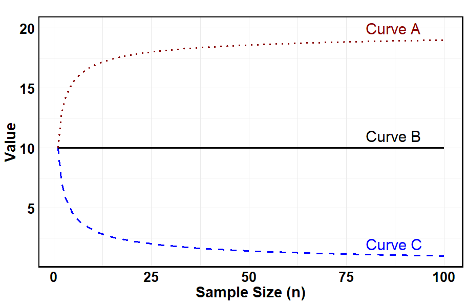
(A) If the distribution \(f_W(w)\) is heavily skewed, a larger sample is required to apply the central limit theorem.

(B) Curve A represents the value of \(sd(\bar{W})\) when the central limit theorem is not applicable.

(C) Curve B represents the value of the \(E[\bar{W}]\) for different sample sizes \(n\).

(D) Curve C indicates that the inference on \(\mu_W\) is more accurate as the sample size increases.

Solution

Answer: (B)

• (A) TRUE. A heavily skewed population requires a larger \(n\) before the CLT provides a good normal approximation to \(\bar{W}\).

• (B) FALSE. Curve A increases with \(n\) and approaches ~20. The standard deviation of \(\bar{W}\) is \(\sigma/\sqrt{n} = 10/\sqrt{n}\), which decreases toward 0 as \(n\) increases — this matches Curve C, not Curve A. Curve A could represent the population standard deviation \(\sigma = 10\) plotted before the CLT kicks in, but it does not represent \(sd(\bar{W})\).

• (C) TRUE. \(E[\bar{W}] = \mu = 10\) regardless of sample size. Curve B is the horizontal line at 10, correctly representing this constant value.

• (D) TRUE. Curve C decreases toward 0 as \(n\) increases, consistent with \(sd(\bar{W}) = \sigma/\sqrt{n} \to 0\). Smaller standard error means more accurate inference on \(\mu_W\).

Question 2.2 (3 pts)

In the context of a one-sample procedure for constructing a 99% confidence interval for the population mean \(\mu\), assuming all conditions for inference are met, which quantity is guaranteed to be within the interval?

1. 0     (B) \(\mu\)     (C) \(\sigma\)     (D) \(\bar{x}\)     (E) None of the above

Solution

Answer: (D)

The confidence interval is constructed as \(\bar{x} \pm t_{\alpha/2,\,n-1} \cdot s/\sqrt{n}\), and the sample mean \(\bar{x}\) is always the center of this interval. Therefore \(\bar{x}\) is always contained within the interval.

• (A) 0 is only in the interval if the data support it — not guaranteed.

• (B) \(\mu\) is the unknown parameter we are estimating — a 99% CI contains \(\mu\) in 99% of repeated samples, but not guaranteed for any single interval.

• (C) \(\sigma\) is a standard deviation, not a mean, so there is no reason it would fall inside a CI for \(\mu\).

Question 2.3 (3 pts)

Consider an experiment in which a sample of size 100 is drawn from a population with unknown mean (\(\mu\)) and unknown standard deviation (\(\sigma\)). The experiment is repeated using ten different samples of the same size, and a 99% confidence interval is constructed for the unknown mean from each sample. Once all the intervals are computed, which of the following is always true?

(A) The critical value used to calculate the confidence intervals is the same across the 10 replications of the experiment.

(B) The numerical value at the center of the confidence interval is the same across the 10 replications of the experiment.

3. The margin of error is the same across the 10 replications of the experiment.

(D) Each of the 10 computed confidence intervals contain the true mean (\(\mu\)) with a probability of 0.99.

5. Two or more of the above statements are correct.

Solution

Answer: (A)

Since \(\sigma\) is unknown and all samples have the same size \(n = 100\), we use a t-distribution with \(df = n - 1 = 99\). The critical value \(t_{0.005,\,99}\) depends only on the confidence level and degrees of freedom — both of which are fixed across all 10 replications. Therefore the critical value is the same for all 10 intervals.

• (B) FALSE. The center is \(\bar{x}\), which varies from sample to sample.

• (C) FALSE. The margin of error is \(t^* \cdot s/\sqrt{n}\). While \(t^*\) and \(n\) are fixed, \(s\) varies across samples, so the margin of error varies.

• (D) FALSE. Once a specific interval is computed, it either contains \(\mu\) or it does not — the probability is 0 or 1, not 0.99. The 99% refers to the long-run frequency of the procedure.

• (E) FALSE — only (A) is always true.

Question 2.4 (3 pts)

Which of the following strategies can a researcher use to increase the power of a statistical hypothesis test?

1. Increase the sample size \(n\).

(B) Increase the distance between the null value \(\mu_0\) and the alternative mean \(\mu_A\).

(C) Reduce the population standard deviation \(\sigma\) by controlling extraneous variables.

4. Increase the significance level \(\alpha\) (Acceptable Type I error rate).

5. All of the above.

Solution

Answer: (E)

Power \(= 1 - \beta\) increases when it becomes easier to distinguish \(H_a\) from \(H_0\). All four strategies accomplish this:

• (A) Larger \(n\) reduces the standard error \(\sigma/\sqrt{n}\), making the sampling distribution tighter and the signal-to-noise ratio larger.

• (B) A larger true effect \(|\mu_A - \mu_0|\) moves the alternative distribution further from the null, increasing the probability of falling in the rejection region.

• (C) Smaller \(\sigma\) also reduces the standard error, with the same effect as increasing \(n\).

• (D) Increasing \(\alpha\) expands the rejection region, which directly increases power (at the cost of more Type I errors).

Question 2.5 (3 pts)

Suppose you are estimating a population parameter using two different estimators: Estimator A is unbiased but has high variance, while Estimator B is biased but has low variance. Which of the following statements is TRUE?

1. Estimator A is always preferred because it is unbiased.

2. Estimator B is always preferred because it has low variance.

(C) Neither estimator is useful because both fail to provide accurate estimates of the true population parameter.

(D) Depending on the context, Estimator B may be preferred if its bias is small, and variance is significantly lower than Estimator A’s.

5. Both estimators are equally effective if the sample size is small enough.

Solution

Answer: (D)

The mean squared error (MSE) of an estimator combines both bias and variance: \(\text{MSE} = \text{Bias}^2 + \text{Variance}\). If Estimator B has small bias and substantially lower variance, its MSE may be smaller than Estimator A’s despite being biased. In practice — for example, in ridge regression or shrinkage estimators — a small amount of bias is deliberately introduced to achieve a large reduction in variance, which can improve overall estimation accuracy. Therefore neither unbiasedness alone nor low variance alone is the deciding criterion.

---

Problem 3 (26 points) — Auto-Insurance CLT

Problem 3 Setup

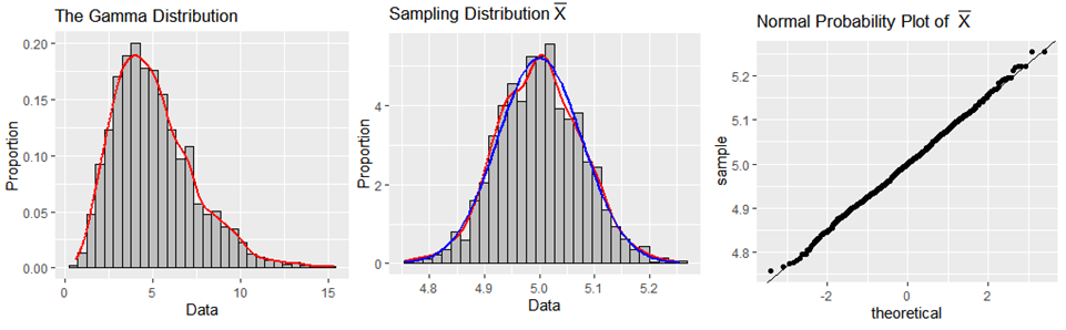
An auto-insurance company plans to adjust policyholders’ premiums based on historical data. According to the data, the claim amounts follow a gamma distribution with a mean of 5k and a standard deviation of 2.25k. The company expects 900 claims to be filed in the upcoming month. These 900 claims can be thought of as a random sample of identically distributed claims drawn from the population distribution of claim amounts. Assume the claims are independent.

An enthusiastic statistician at the company conducted a simulation using 1,500 simple random samples, each of size 900, where each observation was randomly drawn from the gamma distribution. The following graphs are provided to support their analysis of \(\bar{X}\), the average claim amount:

Question 3a (10 pts)

Describe the approximate distribution of \(\bar{X}\), the average claim amount of 900 auto-insurance claims. Provide a detailed justification for why this approximation is valid, including the important theoretical principle that supports your result.

Solution

As indicated by the simulation, the distribution of \(\bar{X}\) will be approximately normal when using samples of size 900 from a population distributed as a gamma distribution with parameters defined as functions of the mean of 5k and the standard deviation of 2.25k.

This is justified by the Central Limit Theorem (CLT): for a sufficiently large sample size \(n\), the sampling distribution of \(\bar{X}\) is approximately normal regardless of the shape of the population distribution. With \(n = 900\), the CLT applies comfortably even for the strongly right-skewed gamma distribution.

This is clearly demonstrated by the simulation evidence:

• The histogram of the 1,500 sample means looks bell-shaped.

• The normal curve (blue) and the kernel density curve (red) have much overlap.

• The normal probability plot for the sample means has only minor deviations at the tails, indicating that normality is a reasonable assumption.

• There are no serious outliers flagged in the histogram or normal probability plots.

Question 3b (3 pts)

Find the mean and standard deviation of the sampling distribution of \(\bar{X}\).

Solution

\[\mu_{\bar{X}} = \mu = \boxed{5 \text{k}}\]

\[\sigma_{\bar{X}} = \frac{\sigma}{\sqrt{n}} = \frac{2.25}{\sqrt{900}} = \frac{2.25}{30} = \boxed{0.075 \text{k}}\]

Question 3c (3 pts)

Select the correct code for determining the probability that the average of 900 claims would be greater than 5.15k.

# (A) pnorm(5.15, mean = 5, sd = 2.25, lower.tail = FALSE)
# (B) pnorm(5.15, mean = 5, sd = 2.25, lower.tail = TRUE)
# (C) pnorm(5.15, mean = 5, sd = 0.075, lower.tail = FALSE)
# (D) pnorm(5.15, mean = 5, sd = 0.075, lower.tail = TRUE)
# (E) pgamma(5.15, shape = 5, rate = 2.25, lower.tail = FALSE)
# (F) pgamma(5.15, shape = 5, rate = 2.25, lower.tail = TRUE)

Solution

Answer: (C)

We need \(P(\bar{X} > 5.15)\) where \(\bar{X} \sim \text{Normal}(5, 0.075)\) approximately by the CLT. The correct code uses the sampling distribution parameters — mean = 5 and standard deviation = 0.075 (the standard error, not the population standard deviation 2.25) — with lower.tail = FALSE for an upper-tail probability.

• 1. and (B) use the population SD 2.25 instead of the standard error 0.075 — incorrect.

• 4. uses the correct SD but wrong tail direction.

• 5. and (F) use a gamma distribution, which applies to individual claims, not to \(\bar{X}\).

Question 3d (10 pts)

Suppose only 10 claims are expected in the upcoming month. Can the same inference about the average claim be made in this case? Justify your answer based on relevant theoretical principles.

Solution

No, the same inference cannot safely be made with only \(n = 10\) claims.

The distribution of \(\bar{X}\) is determined both by the shape of the population and the sample size \(n\). The population of claim amounts follows a gamma distribution, which is strongly positively skewed. With only \(n = 10\) claims, the Central Limit Theorem does not provide a reliable normal approximation — a significantly larger sample size is required for the CLT to apply to a heavily skewed distribution.

Therefore, the approximate normal distribution for \(\bar{X}\) cannot be assumed when \(n = 10\). To determine the probability that the average of 10 claims would be greater than 5.15k, we would need to determine the exact distribution of \(\bar{X}\) (which is a scaled gamma distribution for independent gamma observations) or use other techniques.

---

Problem 4 (25 points) — GreatNotes Algorithm Generalization

Problem 4 Setup

GreatNotes is developing software that converts handwritten mathematical notations into typed text. To evaluate its performance, the company used 200 images of handwritten mathematical equations. Of these, 100 images were included in the training dataset, paired with their correct typed formats. The remaining 100 images were withheld from training to serve as a test set of new, unseen data.

After training, the company tested the algorithm on all 200 images, comparing each algorithm-generated output to its corresponding correct typed format to assess accuracy.

Each output was scored for accuracy, with scores ranging from 0 to 100. A numerical summary of the results is provided below:

	Training Data	Withheld Data	Training − Withheld
\(n\)	100	100	100
Sample Mean	96.4	95.2	1.2
Sample Standard Deviation	2.3	4.5	4.3

It is common for handwriting recognition algorithms to achieve higher accuracy on data used during training. However, for commercial success, GreatNotes must ensure that the algorithm performs comparably on new, unseen data. They will conclude that the algorithm fails to generalize if the true mean accuracy on training data is significantly higher than the true mean accuracy on withheld data.

Using a 91% confidence level, perform a hypothesis test to determine whether the algorithm fails to generalize.

Question 4a (2 pts)

Which two-sample method should be used?

1. Two-sample Independent Procedure

2. Two-sample Paired Procedure

Solution

Answer: (B) Two-sample Paired Procedure

Each image appears in exactly one group (training or withheld), but the 200 images were selected and processed together, with training images matched to withheld images. The summary table provides a Training − Withheld difference column (\(n = 100\), \(\bar{d} = 1.2\), \(s_D = 4.3\)), confirming that each training observation is paired with a corresponding withheld observation.

Question 4b (5 pts)

Perform the first two steps of the four-step hypothesis test.

Solution

Step 1 — Parameters of interest:

The population parameters of interest are \(\mu_\text{Train}\) and \(\mu_\text{Withheld}\), which reflect the algorithm’s true mean accuracy on all potential training images of handwritten mathematical equations and all potential withheld (test) images of handwritten mathematical equations, respectively.

Step 2 — Hypotheses:

\[H_0: \mu_\text{Train} - \mu_\text{Withheld} \leq 0\]

\[H_a: \mu_\text{Train} - \mu_\text{Withheld} > 0\]

Question 4c (8 pts)

Compute the test statistic. Show work.

Solution

Grading Note ⚠️

The solution key selects (B) Paired for Question 4a but computes the test statistic below using the Welch independent two-sample formula — which gives \(t_\text{TS} = 2.3745\) with \(df = 147.42\). The consistent paired t-test applied to the difference column (\(\bar{d} = 1.2\), \(s_D = 4.3\), \(n = 100\)) would give \(t = 1.2 / (4.3/\sqrt{100}) = 2.7907\) with \(df = 99\). The solution below follows the key exactly as graded.

\[t_\text{TS} = \frac{\bar{x}_\text{Train} - \bar{x}_\text{Withheld}}{\sqrt{\dfrac{s_\text{Train}^2}{n_\text{Train}} + \dfrac{s_\text{Withheld}^2}{n_\text{Withheld}}}}\]

\[t_\text{TS} = \frac{96.4 - 95.2}{\sqrt{\dfrac{2.3^2}{100} + \dfrac{4.5^2}{100}}} = \frac{1.2}{\sqrt{0.0529 + 0.2025}} = \frac{1.2}{\sqrt{0.2554}} = \frac{1.2}{0.5054} = \boxed{2.3745}\]

Question 4d (3 pts)

Select the R code that would correctly compute the \(p\)-value.

# (A) pnorm(test_statistic, lower.tail = TRUE)
# (B) pt(test_statistic, df=147.42, lower.tail = TRUE)
# (C) pt(test_statistic, df=199,    lower.tail = TRUE)
# (D) pnorm(test_statistic, lower.tail = FALSE)
# (E) pt(test_statistic, df=147.42, lower.tail = FALSE)
# (F) pt(test_statistic, df=199,    lower.tail = FALSE)

Solution

Answer: (E) pt(test_statistic, df=147.42, lower.tail = FALSE)

This is a right-tailed test (\(H_a: \mu_\text{Train} - \mu_\text{Withheld} > 0\)), so we need the upper-tail probability (lower.tail = FALSE). The degrees of freedom \(df = 147.42\) come from the Welch–Satterthwaite approximation consistent with the test statistic computed in part (c).

Question 4e (7 pts)

The resulting \(p\)-value was approximately 0.009. Provide the formal decision and interpret the conclusion in the context of the problem.

Solution

Decision: The \(p\)-value \(\approx 0.009 < \alpha = 0.09\), therefore we have sufficient evidence to reject \(H_0\).

Conclusion: The data give support (\(p\)-value \(\approx 0.009\)) to the claim that the software fails to generalize — in other words, the true mean accuracy on training data is higher than the true mean accuracy on the withheld data in the population.

Note that this does not assess the practical significance, nor does it indicate that the software is worthless.

---

Problem 5 (27 points) — Coyote Lengths in Georgia

Problem 5 Setup

Urbanization has been associated with an increase in coyote sightings in Georgia (Mowry et al., 2020). This has raised concerns about the role of coyotes in urban ecosystems, particularly regarding human-coyote conflicts and negative interactions with pets.

Residents of Atlanta, GA, believe that coyotes are large on average, with a mean length of at least 94 cm. However, the Georgia Department of Natural Resources (DNR) suspects that the true mean length is less than 94 cm. To investigate, the DNR staff used Geographic Information Systems (GIS) to identify and randomly select sampling locations, supplemented by satellite imagery to capture 29 images of coyotes. From these images, they measured the lengths of the coyotes.

The sample mean length was 89.17 cm. Based on historical data, the DNR has determined that coyote lengths follow a normal distribution with a standard deviation of 9 cm.

Question 5a (8 pts)

Calculate an appropriate 90% confidence interval or bound to assess the belief of the true mean length of coyotes by the Georgian DNR. Clearly specify which R output from the last page of the exam you used.

Solution

Since the DNR suspects the true mean is less than 94 cm, the appropriate confidence region is a 90% upper confidence bound — it gives the highest plausible value for \(\mu_\text{Length}\) and is aligned with the one-sided hypothesis of interest.

Since \(\sigma = 9\) cm is known, we use a \(z\)-based bound.

Using Output 8: qnorm(p=0.1, lower.tail = FALSE) gives \(z_{0.1} = 1.281552\).

\[\text{UCB} = \bar{x}_\text{Length} + z_{0.1} \cdot \frac{\sigma}{\sqrt{n}} = 89.17 + 1.281552 \times \frac{9}{\sqrt{29}} = 89.17 + 1.281552 \times 1.6713 = \boxed{91.3118 \text{ cm}}\]

Question 5b (5 pts)

Interpret the results obtained from part (a) within the context of the problem.

Solution

We are 90% confident that the true mean length of coyotes in Georgia is less than 91.3118 cm.

Since this upper bound (91.3118 cm) is well below the residents’ claimed value of 94 cm, the confidence bound supports the DNR’s suspicion that the true mean coyote length is less than 94 cm.

Question 5c (14 pts)

Carry out a hypothesis test on whether the data supports the claim made by the DNR staff. Use the information from above and on the last page of the exam to perform the four-step hypothesis test. Clearly specify which R output from the last page of the exam was used to obtain your conclusion. Test at \(\alpha = 0.1\).

Question 5 Code/Output:

# Output 1
t.test(coyote_data, conf.level = 0.90, alternative = "greater", mu = 89.17)
# t = 0.0012646, df = 28, p-value = 0.4995

# Output 2
t.test(coyote_data, conf.level = 0.90, alternative = "less", mu = 94)
# t = -2.5293, df = 29, p-value = 0.008671

# Output 3
t.test(coyote_data, conf.level = 0.90, alternative = "two.sided", mu = 94)
# t = -2.5293, df = 28, p-value = 0.01734

# Output 4
z_TS <- (89.17 - 94) / 9
# Test Statistic is: -0.5366667
p_value <- pnorm(z_TS, lower.tail = TRUE)
# p-value is: 0.2957489

# Output 5
z_TS <- (89.17 - 94) / (9 / sqrt(29))
# Test Statistic is: -2.890038
p_value <- pnorm(z_TS, lower.tail = TRUE)
# p-value is: 0.001925974

# Output 6
z_TS <- (89.17 - 94) / 9
# Test Statistic is: -0.5366667
p_value <- 2 * pnorm(z_TS, lower.tail = TRUE)
# p-value is: 0.5914979

# Output 7
z_TS <- (89.17 - 94) / (9 / sqrt(29))
# Test Statistic is: -2.890038
p_value <- 2 * pnorm(z_TS, lower.tail = TRUE)
# p-value is: 0.003851947

# Output 8
# qnorm(p=0.05, lower.tail = TRUE)   -> -1.644854
# qt(p=0.05, df=28, lower.tail=FALSE) -> 1.701131
# qnorm(p=0.1, lower.tail=FALSE)     -> 1.281552
# qt(p=0.1, df=28, lower.tail=FALSE)  -> 1.312527
# qnorm(p=0.1, lower.tail=TRUE)      -> -1.281552
# qt(p=0.1, df=28, lower.tail=TRUE)   -> -1.312527
# qnorm(p=0.05, lower.tail=FALSE)    -> 1.644854
# qt(p=0.05, df=28, lower.tail=TRUE)  -> -1.701131

Solution

Step 1 — Parameter of interest:

Let \(\mu_\text{Length}\) represent the true mean length (in cm) of coyotes in Georgia.

Step 2 — Hypotheses:

\[H_0: \mu_\text{Length} \geq 94 \text{ cm}\]

\[H_a: \mu_\text{Length} < 94 \text{ cm}\]

Step 3 — Test statistic and p-value:

Since \(\sigma = 9\) cm is known and coyote lengths follow a normal distribution, we use a z-test:

\[z_\text{TS} = \frac{\bar{x}_\text{Length} - \mu_0}{\sigma / \sqrt{n}} = \frac{89.17 - 94}{9/\sqrt{29}} = \frac{-4.83}{1.6713} = -2.8900\]

Using Output 5:

z_TS <- (89.17 - 94) / (9 / sqrt(29))
# Test Statistic is: -2.890038
p_value <- pnorm(z_TS, lower.tail = TRUE)
# p-value is: 0.001925974

\(p\text{-value} = P(Z < -2.8900) = 0.0019\)

Step 4 — Decision and conclusion:

Since \(p\text{-value} = 0.001925974 \leq \alpha = 0.1\), we reject \(H_0\).

The data give strong support (\(p\text{-value} = 0.001925974\)) to the claim that the true mean length of coyotes in Georgia is less than 94 cm.