STAT 350 — Exam 2 — Fall 2025

Exam Information

Course: STAT 350 — Introduction to Statistics

Semester: Fall 2025

Total Points: 105

Time Allowed: 60 minutes

Problem	Total Possible	Topic
Problem 1 (True/False, 2 pts each)	12	CLT, Sampling Distributions, Experimental Design, Inference
Problem 2 (Multiple Choice, 3 pts each)	15	Estimation Bias, Estimator Properties, Two-Sample Procedures, Power
Problem 3	27	Two-Sample Paired t-test
Problem 4	28	One-Sample z-test, Power Analysis, Sample Size
Problem 5	23	Sampling Distributions, Normal Population
Total	105

---

Problem 1 — True/False (12 points, 2 points each)

Question 1.1 (2 pts)

Assume that \(X_1, X_2, \cdots, X_n\) is a random sample from a Cauchy distribution, which has an undefined expected value and variance (i.e., \(E[X_i]\) and \(\text{Var}(X_i)\) are not finite).

True or False: Performing a one-sample hypothesis test for the population mean (\(\mu\)) is valid if the sample size (\(n\)) is sufficiently large.

Solution

Answer: FALSE

The Central Limit Theorem requires finite mean and variance. The Cauchy distribution has neither a finite mean nor a finite variance, so the CLT does not apply regardless of sample size. Without the CLT or an underlying normal population, the sampling distribution of \(\bar{X}\) does not converge to a normal distribution, and standard z- or t-based hypothesis tests for \(\mu\) are not valid. In fact, the Cauchy distribution has no well-defined population mean \(\mu\) to test.

Question 1.2 (2 pts)

The lengths of pregnancies are normally distributed with a mean of 268 days and a standard deviation of 15 days.

True or False: Then the probability that a randomly selected pregnant woman’s pregnancy length is less than 265 is larger than the probability that the mean pregnancy length of a random sample of 40 pregnant women is less than 265.

Solution

Answer: TRUE

For an individual observation \(X \sim N(268, 15^2)\):

\[P(X < 265) = P\!\left(Z < \frac{265 - 268}{15}\right) = P(Z < -0.20) = 0.4207\]

For the sample mean \(\bar{X} \sim N\!\left(268,\ (15/\sqrt{40})^2\right)\):

\[P(\bar{X} < 265) = P\!\left(Z < \frac{265 - 268}{15/\sqrt{40}}\right) = P(Z < -1.265) = 0.1029\]

Since \(0.4207 > 0.1029\), the probability for a single observation is larger than for the sample mean. The sample mean has much less variability (\(\sigma/\sqrt{n} = 15/\sqrt{40} \approx 2.37\) vs. \(\sigma = 15\)), so it is much less likely to fall far from the population mean.

Question 1.3 (2 pts)

In experimental design, researchers often encounter extraneous variables that may influence the response variable alongside the factor of interest.

True or False: In a Randomized Block Design (RBD), blocks are used to control the factor of interest, while randomization controls extraneous variables.

Solution

Answer: FALSE

The statement has the roles reversed. In an RBD, blocks are used to control extraneous variables (by grouping experimental units that are similar on a known nuisance factor), while randomization is used to assign the factor of interest (treatments) to units within each block. Blocks reduce the impact of extraneous variability; randomization ensures unbiased treatment comparison.

Question 1.4 (2 pts)

A researcher conducts a hypothesis test and obtains a \(p\)-value of 0.03.

True or False: This means there is a 3% probability that the null hypothesis is true.

Solution

Answer: FALSE

The \(p\)-value is not the probability that \(H_0\) is true. The \(p\)-value is the probability of observing a test statistic at least as extreme as the one obtained, assuming \(H_0\) is true. It is a statement about the data given the hypothesis, not about the hypothesis given the data. The null hypothesis is either true or false — it does not have a probability in the classical (frequentist) framework.

Question 1.5 (2 pts)

A 95% confidence interval for the population mean \(\mu\) is constructed from sample data.

True or False: A sample mean \(\bar{x}\) falls within the 95% confidence interval for all possible samples from the population.

Solution

Answer: TRUE

A confidence interval is always constructed as \(\bar{x} \pm t^* \cdot s/\sqrt{n}\), centered at the sample mean \(\bar{x}\). Therefore, by construction, \(\bar{x}\) is always the center of the interval and is contained within it for every possible sample.

Question 1.6 (2 pts)

A researcher wants to estimate the average income in a city with diverse neighborhoods.

True or False: In a stratified random sample, the city is divided into neighborhoods (strata), and then a few complete neighborhoods are randomly selected and all residents within those neighborhoods are surveyed.

Solution

Answer: FALSE

The description given is cluster sampling, not stratified sampling. In a stratified random sample, the population is divided into strata, and then a random sample is drawn from within each stratum. In cluster sampling, a few clusters (e.g., complete neighborhoods) are randomly selected and all units within the chosen clusters are surveyed. The key distinction: stratified sampling samples from every stratum; cluster sampling surveys all units in only a few selected clusters.

---

Problem 2 — Multiple Choice (15 points, 3 points each)

Question 2.1 (3 pts)

A student proposes an estimator for an unknown parameter \(\theta\). The estimator \(\hat{\theta}\) has expected value \(E[\hat{\theta}] = \left(\dfrac{n}{n-1}\right)\theta + 5\), where \(n\) is the sample size. What is the exact bias (for finite \(n\)) and the asymptotic bias as \(n \to \infty\) of this estimator?

1. Exact bias \(= 5\); Asymptotic bias \(= 0\)

2. Exact bias \(= \left(\dfrac{1}{n-1}\right)\theta\); Asymptotic bias \(= 5\)

3. Exact bias \(= \left(\dfrac{1}{n-1}\right)\theta + 5\); Asymptotic bias \(= 5\)

4. Exact bias \(= \left(\dfrac{1}{n-1}\right)\theta + 5\); Asymptotic bias \(= 0\)

5. Exact bias \(= \left(\dfrac{n}{n-1}\right)\theta + 5\); Asymptotic bias \(= \theta\)

Solution

Answer: (C)

The bias of an estimator is \(\text{Bias}(\hat{\theta}) = E[\hat{\theta}] - \theta\).

Exact bias:

\[\text{Bias}(\hat{\theta}) = \frac{n}{n-1}\,\theta + 5 - \theta = \left(\frac{n}{n-1} - 1\right)\theta + 5 = \frac{1}{n-1}\,\theta + 5\]

Asymptotic bias as \(n \to \infty\):

\[\lim_{n \to \infty} \left(\frac{1}{n-1}\,\theta + 5\right) = 0 + 5 = 5\]

The \(\theta/(n-1)\) term vanishes but the constant additive bias of 5 remains, so the estimator is asymptotically biased by 5.

Question 2.2 (3 pts)

Three estimators, \(\hat{\theta}_A\), \(\hat{\theta}_B\), \(\hat{\theta}_C\), are constructed for an unknown target parameter \(\theta\), and their sampling distributions are visualized in the graph below. Which of the following statements is TRUE about the estimators?

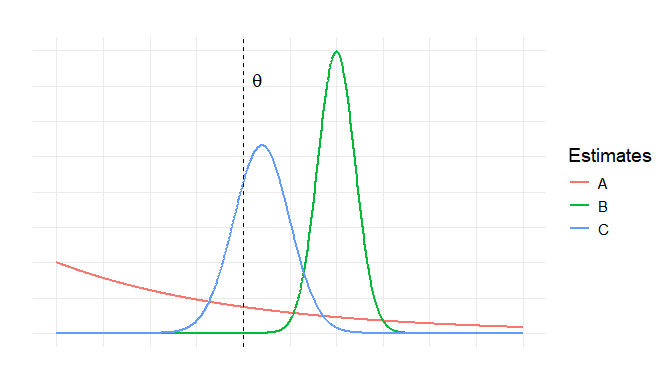
(A) \(\hat{\theta}_B\) is preferred over \(\hat{\theta}_A\) because \(\hat{\theta}_B\) has a smaller variance.

(B) \(\hat{\theta}_A\) is preferred over \(\hat{\theta}_C\) if \(\hat{\theta}_A\) has a smaller bias.

(C) \(\hat{\theta}_C\) is preferred over \(\hat{\theta}_A\) even if \(\hat{\theta}_A\) has a smaller bias.

(D) On repeated samples, \(\hat{\theta}_A\) values hardly vary around the true parameter.

5. The best estimate can be determined only after obtaining realized values.

Solution

Answer: (C)

From the graph: Curve A (red) is wide and flat — high variance, biased. Curve B (green) is tall and narrow but shifted right of \(\theta\) — low variance, biased. Curve C (blue) is moderate width and centered at \(\theta\) — unbiased, moderate variance.

• (A) FALSE. \(\hat{\theta}_B\) does have smaller variance than \(\hat{\theta}_A\), but preference cannot be determined by variance alone — the bias matters too. \(\hat{\theta}_B\) is biased.

• (B) FALSE. Even if \(\hat{\theta}_A\) had smaller bias than \(\hat{\theta}_C\), its extremely high variance (flat, wide curve) would likely give it a larger MSE than \(\hat{\theta}_C\).

• (C) TRUE. \(\hat{\theta}_C\) is unbiased and has moderate variance. Even if \(\hat{\theta}_A\) were somehow less biased, its very large variance means its MSE would likely exceed \(\hat{\theta}_C\)’s. The MSE combines both bias and variance; \(\hat{\theta}_C\)’s combination is superior.

• (D) FALSE. \(\hat{\theta}_A\) is the wide, flat curve — it has the largest variance, meaning values vary greatly around \(\theta\) on repeated samples.

• (E) FALSE. The best estimator is evaluated based on the properties of the sampling distributions (bias, variance, MSE), not after seeing individual realized values.

Question 2.3 (3 pts)

Two fertilizers are tested on different plots to compare their effects on crop yield. Summary statistics: \(n_1 = 22\), \(s_1 = 19.5\) kg/hectare and \(n_2 = 20\), \(s_2 = 4.7\) kg/hectare. Which statistical inference procedure is most appropriate for comparing mean yields?

1. One-sample \(t\)-procedures

2. Two-sample paired \(t\)-procedures

3. Pooled two-sample independent \(t\)-procedures

4. Welch two-sample independent \(t\)-procedures

Solution

Answer: (D)

The two groups (fertilizer 1 vs. fertilizer 2) are tested on different plots — there is no pairing or matching, so independent-samples procedures are required. The sample standard deviations are \(s_1 = 19.5\) and \(s_2 = 4.7\), a ratio of more than 4:1. This large difference in variability makes the equal-variance (pooled) assumption inappropriate. The Welch two-sample independent t-procedure does not require equal variances and is therefore the most appropriate choice.

Question 2.4 (3 pts)

A researcher wants to test the effect of a new type of feed on the weight gain of chickens. They have 100 chickens, but they are housed in 10 different coops (10 chickens per coop). The researcher knows that conditions (like temperature and lighting) vary slightly between coops, which might affect weight gain. To account for this, the researcher randomly assigns 5 chickens within each coop to the new feed and the other 5 to the standard feed.

Which experimental design technique is demonstrated by separating the chickens by coop before assigning the feed?

1. Completely Randomized Design     (B) Randomized Block Design     (C) Simple Random Sample     (D) Matched Pairs Design     (E) Stratified Random Sampling

Solution

Answer: (B) Randomized Block Design

The coops serve as blocks — groups of experimental units (chickens) that are homogeneous with respect to a known extraneous variable (coop conditions: temperature and lighting). Within each block (coop), treatments (new feed vs. standard feed) are randomly assigned. This is the defining structure of a Randomized Block Design: blocking on the extraneous variable before randomizing treatments within blocks.

Question 2.5 (3 pts)

Chloride deposits are markers for early Mars’ aqueous past with important implications for our understanding of Mars’ climate and habitability. Purdue scientists are in the process of investigating high-resolution image surfaces of 33 chloride deposits from the southern highlands of Mars. Researchers from a different university have claimed that the mean diameter of chloride deposits is 1650 m with the standard deviation of 779.42 m. Studies of geological features suggest that the diameters of natural deposits tend to follow approximately symmetric distributions. Based on the Central Limit Theorem and assuming the other researchers’ claim correctly describes the population, which of the following statements is incorrect?

(A) The standard deviation of the sampling distribution of \(\bar{X}\) for Purdue investigations should be 779.42 m.

(B) The mean of the sampling distribution of \(\bar{X}\) for Purdue investigations is 1650 m.

(C) The sampling distribution of \(\bar{X}\) for Purdue investigations is approximately normal.

4. We cannot assume the population distribution of deposit diameters is exactly normal.

Solution

Answer: (A)

The standard deviation of the sampling distribution of \(\bar{X}\) is the standard error, not the population standard deviation:

\[\sigma_{\bar{X}} = \frac{\sigma}{\sqrt{n}} = \frac{779.42}{\sqrt{33}} \approx 135.68 \text{ m}\]

Statement (A) incorrectly claims \(\sigma_{\bar{X}} = 779.42\) m, which is the population standard deviation. The remaining statements are all correct:

• (B) \(\mu_{\bar{X}} = \mu = 1650\) m — always true.

• (C) With \(n = 33\) and a symmetric population, the CLT gives approximate normality for \(\bar{X}\).

• (D) The population is described as approximately symmetric but not stated to be exactly normal, so this caveat is correct.

---

Problem 3 (27 points) — Coffee Roasting Machine Moisture Test

Problem 3 Setup

A coffee company is testing a new, faster roasting machine. The old machine roasts beans to a target mean moisture level of 8.0%. The company suspects the new machine (N) produces a different mean moisture level than the old machine (O).

They conduct an experiment. They take 16 batches of the same type of green coffee bean. For each batch, they split it in half, roasting one half with the new machine and the other half with the old machine. The moisture level for each roasted half is recorded.

The company calculates the difference for each batch: \(D = \text{Moisture}_N - \text{Moisture}_O\). The data for the 16 differences yields a sample mean difference of 0.25% and a standard deviation of differences of 0.60%. The researchers have verified that the distribution of differences is approximately normal.

Question 3a (2 pts)

Which testing procedure is appropriate for this experiment?

1. Two-sample independent \(t\)-test

2. Two-sample paired \(t\)-test

Solution

Answer: (B) Two-sample paired t-test

Question 3b (4 pts)

Explain what characteristic(s) in the experimental design motivated your choice of testing procedure in part (a).

Solution

Each batch is split into two halves, with each half roasted using a different machine. This means the two measurements within a batch are not independent — they share the same batch characteristics (bean type, initial moisture content, batch size, etc.). Because each pair of observations (one from the new machine, one from the old machine) comes from the same batch, the observations are paired by batch. The paired \(t\)-test accounts for this within-batch dependence by analyzing the differences \(D_i\) directly, thereby controlling for batch-to-batch variability.

Question 3c (2 pts)

Provide the first two steps of the four-step hypothesis testing procedure.

Solution

Step 1 — Parameter of interest:

Let \(\mu_D = \mu_{\text{Moisture}_N} - \mu_{\text{Moisture}_O}\) represent the true population mean moisture difference associated with roasting from the two machines (New − Old).

Step 2 — Hypotheses:

\[H_0: \mu_D = 0\]

\[H_a: \mu_D \neq 0\]

Question 3d (10 pts)

Calculate the test statistic for this test. Show your work.

Solution

\[t_\text{TS} = \frac{\bar{D} - 0}{s_D / \sqrt{n}} = \frac{0.25}{0.60 / \sqrt{16}} = \frac{0.25}{0.60 / 4} = \frac{0.25}{0.15} = \boxed{1.6667}\]

Degrees of freedom: \(df = n - 1 = 15\).

Question 3e (3 pts)

Select the appropriate code to compute the \(p\)-value below.

# (A) pt(test_statistic, df=15, lower.tail=TRUE)
# (B) 2*pt(abs(test_statistic), df=15, lower.tail=TRUE)
# (C) 2*pt(abs(test_statistic), df=15, lower.tail=FALSE)
# (D) pt(test_statistic, df=15, lower.tail=FALSE)
# (E) pt(test_statistic, df=25.8734, lower.tail=TRUE)
# (F) 2*pt(abs(test_statistic), df=25.8734, lower.tail=TRUE)
# (G) 2*pt(abs(test_statistic), df=25.8734, lower.tail=FALSE)
# (H) pt(test_statistic, df=25.8734, lower.tail=FALSE)

Solution

Answer: (C) 2*pt(abs(test_statistic), df=15, lower.tail=FALSE)

This is a two-sided test (\(H_a: \mu_D \neq 0\)). The \(p\)-value is twice the upper-tail probability beyond the absolute value of the test statistic. The degrees of freedom for a paired t-test on \(n = 16\) pairs is \(df = n - 1 = 15\). The Welch df of 25.8734 (options E–H) would apply to an independent two-sample test, which is not appropriate here.

Question 3f (6 pts)

The \(p\)-value for the correct test was found to be 0.1805. Using a significance level of \(\alpha = 0.1\), state your formal decision and write a conclusion in the context of the problem.

Note on p-value ⚠️

The \(p\)-value reported in the solution key (0.1805) does not match the computed test statistic. With \(t_\text{TS} = 1.6667\) and \(df = 15\), the correct \(p\)-value is \(2 \times P(T_{15} > 1.6667) = \mathbf{0.1163}\). Both values lead to the same decision (fail to reject at \(\alpha = 0.10\)), so the conclusion is unaffected. The solution below uses the key’s reported value of 0.1805.

Solution

Formal Decision: \(p\text{-value} = 0.1805 > 0.1 = \alpha\), therefore we fail to reject \(H_0\).

Conclusion: The data do not give support (\(p\)-value \(= 0.1805\)) to the claim that the true mean difference in moisture levels produced by roasting from the two machines differs from 0.

---

Problem 4 (28 points) — Cranberry Farm pH Test

Problem 4 Setup

Jamie owns a small cranberry farm that primarily grows the Stevens variety, which is known for being sweeter and less tart than Early Black. Recently, he planted a small patch of Early Black cranberries for his daughter, who loves tart berries. After a few years, some regular customers have claimed that the Stevens cranberries have become more tart.

Jamie wants to test whether the presence of Early Black cranberries has caused an increase in tartness of his cranberries. Industry standards indicate that pH measurements from Stevens cranberry batches have an average pH of 2.6 with a standard deviation of 0.3. Research indicates that most people can detect a pH change of 0.2 (lower pH = more tart).

Question 4a (2 pts)

Provide the first two steps of the four-step hypothesis testing procedure.

Solution

Step 1 — Parameter of interest:

Let \(\mu\) represent the true population mean tartness (pH) of Stevens cranberry batches from Jamie’s farm.

Step 2 — Hypotheses:

\[H_0: \mu \geq 2.6\]

\[H_a: \mu < 2.6\]

Question 4b (2 pts)

Identify the mean and standard deviation of the sampling distribution of \(\bar{X}\) under the null and alternative hypotheses to detect a pH change of 0.2. Since the sample size is currently unknown you may use \(n\) to represent it.

Solution

Under \(H_0\):

\[\bar{X} \sim N\!\left(\mu_0 = 2.6,\ \sigma_{\bar{X}} = \frac{0.3}{\sqrt{n}}\right)\]

Under \(H_a\) (to detect a change of 0.2 toward more tartness):

\[\bar{X} \sim N\!\left(\mu_a = 2.4,\ \sigma_{\bar{X}} = \frac{0.3}{\sqrt{n}}\right)\]

Question 4c (10 pts)

Calculate the minimum sample size required to achieve 90% statistical power for detecting a pH difference of 0.2 in the direction that would indicate increased tartness at \(\alpha = 0.04\). Show your work and clearly identify both: (i) the critical \(z\)-value for your significance level, and (ii) the critical \(z\)-value for your desired power.

qnorm(0.01, lower.tail = FALSE)  # 2.326348
qnorm(0.02, lower.tail = FALSE)  # 2.053749
qnorm(0.04, lower.tail = FALSE)  # 1.750686
qnorm(0.05, lower.tail = FALSE)  # 1.644854
qnorm(0.1,  lower.tail = FALSE)  # 1.281552
qnorm(0.2,  lower.tail = FALSE)  # 0.8416212

Solution

(i) Critical z-value for \(\alpha = 0.04\) (left-tailed test):

\[z_\alpha = \texttt{qnorm(0.04, lower.tail = FALSE)} = 1.750686\]

(ii) Critical z-value for 90% power (\(\beta = 0.10\)):

\[z_\beta = \texttt{qnorm(0.1, lower.tail = FALSE)} = 1.281552\]

Cutoff expression:

\[\bar{x}_\text{cutoff} = \mu_0 - z_\alpha \cdot \frac{\sigma}{\sqrt{n}} = 2.6 - 1.750686 \cdot \frac{0.3}{\sqrt{n}}\]

Power condition:

Setting \(P(\bar{X} < \bar{x}_\text{cutoff} \mid \mu = 2.4) = 0.90\):

\[\frac{\bar{x}_\text{cutoff} - \mu_a}{\sigma/\sqrt{n}} = -z_\beta \qquad \Longrightarrow \qquad \frac{\mu_0 - z_\alpha \cdot \frac{\sigma}{\sqrt{n}} - \mu_a}{\sigma/\sqrt{n}} = -z_\beta\]

Rearranging:

\[\sqrt{n} = \frac{(z_\alpha + z_\beta)\,\sigma}{\mu_0 - \mu_a}\]

\[n = \left\lceil\left(\frac{z_\alpha + z_\beta}{(\mu_0 - \mu_a)/\sigma}\right)^2\right\rceil = \left\lceil\left(\frac{1.750686 + 1.281552}{0.2/0.3}\right)^2\right\rceil = \left\lceil\left(\frac{3.032238}{0.6667}\right)^2\right\rceil\]

\[= \left\lceil (4.5484)^2 \right\rceil = \lceil 20.6876 \rceil = \boxed{21}\]

Question 4d (8 pts)

Assume Jamie collects a random sample of 25 cranberry batches and measures the average pH of each batch. Determine the cutoff pH value (\(\bar{x}_\text{cutoff}\)) corresponding to a significance level \(\alpha = 0.04\). Assume the population standard deviation remains \(\sigma = 0.3\) (unchanged from the industry standard). Show your work.

qnorm(0.04, lower.tail = FALSE)  # 1.750686

Solution

Since \(\sigma = 0.3\) is known, we use a \(z\)-based cutoff. For a left-tailed test at \(\alpha = 0.04\):

\[z_\alpha = \texttt{qnorm(0.04, lower.tail = FALSE)} = 1.750686\]

\[\bar{x}_\text{cutoff} = \mu_0 - z_\alpha \cdot \frac{\sigma}{\sqrt{n}} = 2.6 - 1.750686 \times \frac{0.3}{\sqrt{25}} = 2.6 - 1.750686 \times 0.06 = 2.6 - 0.1050 = \boxed{2.4950}\]

Question 4e (3 pts)

Which of the following R code correctly computes the statistical power of the test?

# (A) pnorm((cutoff-2.6)/0.3,  lower.tail=TRUE)
# (B) pnorm((cutoff-2.6)/0.06, lower.tail=TRUE)
# (C) pnorm((cutoff-2.6)/0.06, lower.tail=FALSE)
# (D) pnorm((cutoff-2.4)/0.3,  lower.tail=FALSE)
# (E) pnorm((cutoff-2.4)/0.06, lower.tail=TRUE)
# (F) pnorm((cutoff-2.4)/0.06, lower.tail=FALSE)

Solution

Answer: (E) pnorm((cutoff-2.4)/0.06, lower.tail=TRUE)

Power is the probability of rejecting \(H_0\) when the true mean is \(\mu_a = 2.4\):

\[\text{Power} = P\!\left(\bar{X} < \bar{x}_\text{cutoff} \mid \mu = 2.4\right) = P\!\left(Z < \frac{\bar{x}_\text{cutoff} - 2.4}{\sigma/\sqrt{n}}\right)\]

where \(\sigma/\sqrt{n} = 0.3/\sqrt{25} = 0.06\).

• 1. and (B): subtracts 2.6 (null mean) instead of 2.4 (alternative mean) — wrong.

• (C): same error plus wrong tail direction.

• (D): uses population SD 0.3 instead of standard error 0.06.

• (F): wrong tail — power for left-tailed test requires lower.tail=TRUE.

Question 4f (3 pts)

Which of the following interventions will improve the statistical power of the test, assuming all other factors remain constant? Select all that apply.

1. Plant more Early Black cranberries on the farm.

2. Randomly sample more bags of cranberries from the farm.

3. Move Early Black bushes to a greenhouse with its own beehive.

4. Use a more precise pH measuring device.

Solution

Answers: (B) and (D)

• (A) Does not improve power. Planting more Early Black cranberries would increase cross-pollination, potentially increasing the true effect size — but this changes the experiment itself, not the statistical procedure. The question asks about statistical power holding the effect constant.

• (B) Improves power. A larger sample size \(n\) reduces the standard error \(\sigma/\sqrt{n}\), making it easier to detect a true difference.

• (C) Does not improve power. Moving bushes to a greenhouse reduces cross-pollination and may reduce the true pH change, but does not directly increase statistical power.

• (D) Improves power. A more precise pH measuring device reduces measurement error, which reduces the variability \(\sigma\) in the data. Smaller \(\sigma\) decreases the standard error and increases power.

---

Problem 5 (23 points) — South African Dairy Production

Problem 5 Setup

South Africa contributes significantly to the global dairy market. The most productive provinces are Limpopo and Mpumalanga. Limpopo cows average 27.3 liters of milk a day, with a standard deviation of 2.4 liters. For Mpumalanga cows, the mean daily production is 25.0 liters, with a standard deviation of 3.2 liters. Assume that the milk production for these provinces follow normal distributions.

Question 5a (2 pts)

True or False: We require sample sizes of at least 30 for the sampling distribution of the average daily milk production in both provinces to be approximately Normal.

Solution

Answer: FALSE

Since milk production in both provinces is stated to follow normal distributions, the sampling distribution of \(\bar{X}\) is exactly normal for any sample size \(n \geq 1\) — no CLT approximation is needed. The “at least 30” guideline applies when the population is non-normal and we rely on the CLT.

Question 5b (8 pts)

A random sample of 20 Limpopo cows was selected for a study and an average of 31 liters of milk per day was recorded. How many standard deviations is this average away from its population mean?

Solution

The standard error of \(\bar{X}\) for Limpopo with \(n = 20\) is:

\[\sigma_{\bar{X}} = \frac{\sigma}{\sqrt{n}} = \frac{2.4}{\sqrt{20}} = 0.5367 \text{ liters}\]

The number of standard deviations away from the population mean:

\[z = \frac{\bar{x} - \mu}{\sigma_{\bar{X}}} = \frac{31 - 27.3}{2.4/\sqrt{20}} = \frac{3.7}{0.5367} = \boxed{6.8945}\]

This sample mean is approximately 6.89 standard errors above the population mean — an extremely unlikely result if the population mean is truly 27.3 liters.

Question 5c (10 pts)

A Mpumalanga farmer has 20 cows. There is a 50% chance each day that the total daily production from this herd is at most how many liters? Justify your answer.

Solution

Let \(T = \sum_{i=1}^{20} X_i\) be the total daily production from 20 independent Mpumalanga cows, where \(X_i \sim N(25.0,\ 3.2^2)\).

Since the \(X_i\)’s are i.i.d. normal:

\[T \sim N(\mu_T,\ \sigma_T^2)\]

where:

\[\mu_T = n \cdot \mu = 20 \times 25.0 = 500 \text{ liters}\]

\[\sigma_T^2 = n \cdot \sigma^2 = 20 \times (3.2)^2 = 20 \times 10.24 = 204.8\]

The 50th percentile of any symmetric distribution equals its mean. Since \(T\) is normally distributed:

\[P(T \leq 500) = 0.50\]

There is a 50% chance each day that the total production from a herd of 20 Mpumalanga cows is at most \(\boxed{500 \text{ liters}}\).

Question 5d (3 pts)

A Limpopo farmer has 20 cows. What is the probability that the average milk production for this herd exceeds 38 liters a day?

# (A) pnorm((38-27.3)/2.4,      lower.tail=FALSE)
# (B) 1-pnorm((38-25)/3.2,      lower.tail=TRUE)
# (C) 1-pnorm((38-27.3)/0.5367, lower.tail=TRUE)
# (D) pt((38-27.3)/0.5367, df=19, lower.tail=FALSE)

Solution

Answer: (C) 1-pnorm((38-27.3)/0.5367, lower.tail=TRUE)

We need \(P(\bar{X} > 38)\) where \(\bar{X} \sim N(27.3,\ (2.4/\sqrt{20})^2)\).

The standard error is \(\sigma_{\bar{X}} = 2.4/\sqrt{20} = 0.5367\) liters.

\[P(\bar{X} > 38) = P\!\left(Z > \frac{38 - 27.3}{0.5367}\right) = 1 - \Phi\!\left(\frac{38 - 27.3}{0.5367}\right)\]

In R: 1-pnorm((38-27.3)/0.5367, lower.tail=TRUE)

• (A) Uses the population SD (2.4) instead of the standard error (0.5367).

• (B) Uses Mpumalanga parameters (25, 3.2) instead of Limpopo’s.

• (D) Uses a t-distribution — incorrect since \(\sigma\) is known.