Section 6.8 Reliability and Evaluation

The techniques from previous sections—embedding, annotation, RAG, prompt engineering—are powerful, but they share a critical vulnerability: LLM outputs cannot be blindly trusted. A model that classifies sentiment correctly 85% of the time will introduce systematic errors into any analysis that assumes perfect labels. A RAG system that retrieves the wrong context will generate confidently wrong answers. A model that claims “95% confidence” in an answer that turns out to be incorrect provides worse-than-useless uncertainty information.

For data scientists, unreliable predictions are not merely inconvenient—they threaten the integrity of downstream analyses. Bootstrap confidence intervals computed on LLM-annotated data are only meaningful if the annotations are accurate. Regression models trained on LLM-derived features inherit whatever biases exist in those features. The statistical rigor we developed in Chapters 1–5 is wasted if the inputs are corrupted.

This section develops the tools to measure reliability and quantify uncertainty in LLM outputs. These are not optional add-ons—they are prerequisites for responsibly incorporating LLMs into analytical workflows.

Road Map 🧭

• Identify the three reliability challenges: hallucination, inconsistency, and overconfidence

• Measure consistency through test-retest and paraphrase invariance experiments

• Validate self-consistency as an uncertainty signal—checking whether agreement tracks accuracy, rather than assuming it

• Implement LLM-as-judge evaluation for tasks without ground truth

• Quantify uncertainty using self-consistency and bootstrap interval estimates

• Design complete evaluation protocols for LLM-assisted workflows

The Reliability Challenge

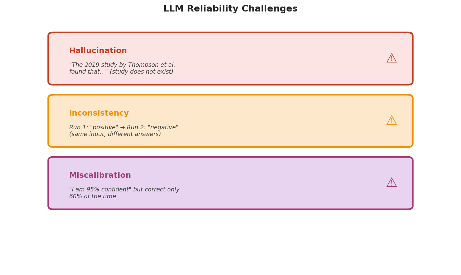
Fig. 242 Figure 6.8.1: The three pillars of LLM unreliability. Hallucination invents facts; inconsistency produces different answers to the same question; overconfidence makes a wrong answer look certain. Each demands different measurement and mitigation strategies.

LLMs are unreliable by default. This is not a bug—it is a consequence of how they work. A model trained to predict the most likely next token will sometimes produce plausible-sounding text that happens to be wrong. Understanding the specific failure modes helps us design targeted mitigations.

Hallucination occurs when a model generates claims not supported by its input or any factual source. This ranges from fabricated citations to invented statistics. RAG (Section 6.5) is the primary mitigation for knowledge-based hallucination.

Inconsistency means the model gives different answers to the same question across runs. LLM generation is inherently stochastic—the model samples each token from a probability distribution, with the amount of randomness governed by server-side sampling settings (such as temperature) that our genai_studio calls leave at their defaults—so repeated queries can yield contradictory results. Self-consistency (Section 6.6) aggregates across runs.

Overconfidence means the model’s apparent certainty does not match its accuracy—it can state, or unshakably repeat, a wrong answer with total assurance. As we will see, any usable uncertainty has to come from the model’s behavior (its consistency across runs), not from asking the model how sure it is—and even then it must be validated against ground truth, not trusted.

Consistency Assessment

Test-Retest Reliability

The simplest consistency check: ask the same question multiple times and measure how often the answer is the same.

from genai_studio import GenAIStudio
from collections import Counter
import numpy as np

ai = GenAIStudio()
ai.select_model("gemma3:12b")

def test_retest(question, prompt_template, n_runs=10):
    """Measure answer consistency across repeated runs."""
    answers = []
    for _ in range(n_runs):
        response = ai.chat(prompt_template.format(question=question))
        answer = response.strip().lower()
        answers.append(answer)

    counter = Counter(answers)
    majority, majority_count = counter.most_common(1)[0]
    agreement = majority_count / n_runs

    return {
        "question": question,
        "majority_answer": majority,
        "agreement": agreement,
        "unique_answers": len(counter),
        "all_answers": answers,
    }

CLASSIFY_PROMPT = """Classify this text as positive, negative, or neutral.
Respond with ONLY one word.

Text: {question}
Label:"""

result = test_retest("The product is decent but a bit overpriced.",
                      CLASSIFY_PROMPT, n_runs=10)
print(f"Question: {result['question']}")
print(f"Majority: {result['majority_answer']} ({result['agreement']:.0%})")
print(f"Unique answers: {result['unique_answers']}")
print(f"All answers: {result['all_answers']}")

Question: The product is decent but a bit overpriced.
Majority: neutral (60%)
Unique answers: 2
All answers: ['neutral', 'negative', 'neutral', 'neutral', 'negative', 'neutral', 'neutral', 'negative', 'negative', 'neutral']

A 60% agreement rate means the model is genuinely uncertain about this ambiguous input. This is valuable information: items with low test-retest reliability should be flagged for human review.

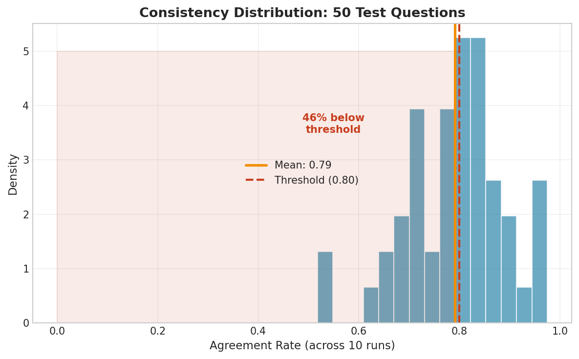
Fig. 243 Figure 6.8.2: Distribution of agreement rates across 50 test questions. Most items achieve high consistency (>80%), but a significant minority falls below the threshold, indicating genuine model uncertainty or task ambiguity.

Paraphrase Invariance

A reliable model should give the same answer regardless of how the question is phrased:

def paraphrase_invariance(paraphrases, annotate_fn):
    """Check if the model gives consistent labels across paraphrases."""
    labels = [annotate_fn(p) for p in paraphrases]
    counter = Counter(labels)
    majority, count = counter.most_common(1)[0]
    return {
        "paraphrases": paraphrases,
        "labels": labels,
        "majority": majority,
        "agreement": count / len(labels),
        "invariant": len(counter) == 1,
    }

paraphrases = [
    "The product quality is good but the price is too high.",
    "Good quality, though it's overpriced.",
    "Quality-wise it's fine, but I paid too much.",
    "Nice product, just wish it were cheaper.",
    "The quality is decent but the cost is steep.",
]

def classify(text):
    return ai.chat(CLASSIFY_PROMPT.format(question=text)).strip().lower()

result = paraphrase_invariance(paraphrases, classify)
print(f"Labels: {result['labels']}")
print(f"Agreement: {result['agreement']:.0%}")
print(f"Invariant: {result['invariant']}")

Labels: ['neutral', 'neutral', 'negative', 'positive', 'negative']
Agreement: 40%
Invariant: False

This reveals a significant reliability problem: semantically equivalent inputs produce different labels. For any analysis relying on these labels, this inconsistency introduces noise that weakens statistical power and may bias results.

Can You Trust a Confidence Number?

It is natural to want a single number for how sure the model is—and tempting to get it by asking. Both the shortcut and the classical tool need care here.

Don’t ask the model. The obvious move is to have the model rate itself—“answer, and give your confidence from 0 to 1.” Resist it. A verbalized confidence is just more generated text: the model produces a plausible-looking number, it does not measure a probability. It has no reliable introspective access to whether its own answer is correct, and empirically—especially for the smaller open models here—these self-reports are poor: they cluster near the top (a model will say “95%” for almost any question), respond only weakly to whether the answer is right, and shift under trivial rewordings. A self-reported “95%” on a wrong answer is worse than useless: it manufactures false certainty.

A reported confidence is not a probability

Asking an LLM “how sure are you?” returns a number the model wrote, not one it computed—it reflects how confident such answers tend to sound in the training data, not this answer’s chance of being right. Treat any self-reported confidence as narrative, not measurement.

And you can’t read a calibrated probability off the model either. A generative LLM answering free-form questions through the gateway does not hand us a probability of being correct: the token probabilities are not exposed, and a self-report is not one. So we will not manufacture a confidence where the model produced none—no diagram drawn over an LLM’s raw answers turns a guess into a measured probability. What we can do is build an uncertainty signal from the model’s behavior and treat it honestly as a heuristic.

Self-consistency is that heuristic—so validate it. The test-retest agreement rate from the previous section is grounded in observed outputs, so it is usable—but it measures stability, not correctness, and the two can come apart:

# Reuse test_retest() from above. The agreement rate is a behavior-based signal —
# but it reports how STABLE the answer is, not whether it is RIGHT.
QA_PROMPT = "Answer in as few words as possible.\n\nQuestion: {question}\nAnswer:"

for q, truth in [("What is the capital of France?", "paris"),
                 ("Who wrote Hamlet?", "shakespeare"),
                 ("In what year did the Berlin Wall fall?", "1989"),
                 ("What is the 12th prime number?", "37")]:
    r = test_retest(q, QA_PROMPT, n_runs=10)
    hit = truth in r["majority_answer"]
    print(f"  [{r['agreement']:.0%} agree] {'OK ' if hit else 'X  '}{q[:38]} -> {r['majority_answer'][:12]}")

[100% agree] OK  What is the capital of France?         -> paris
[ 75% agree] OK  Who wrote Hamlet?                      -> shakespeare
[100% agree] OK  In what year did the Berlin Wall fall? -> 1989
[100% agree] X   What is the 12th prime number?         -> 19

The last line is the whole point: the model is 100% consistent and 100% wrong—unshakably sure the 12th prime is 19 (it is 37). A high agreement rate means the answer is stable, not that it is correct. So use it as a triage signal—route low-agreement items to a human—never as a probability of being right, and always check it against ground truth rather than trusting it on faith. Under Uncertainty Quantification below, we turn this agreement rate into an uncertainty estimate with a bootstrap interval.

LLM-as-Judge

For tasks without ground-truth labels—open-ended generation, summarization, explanation quality—we can use one LLM to evaluate another.

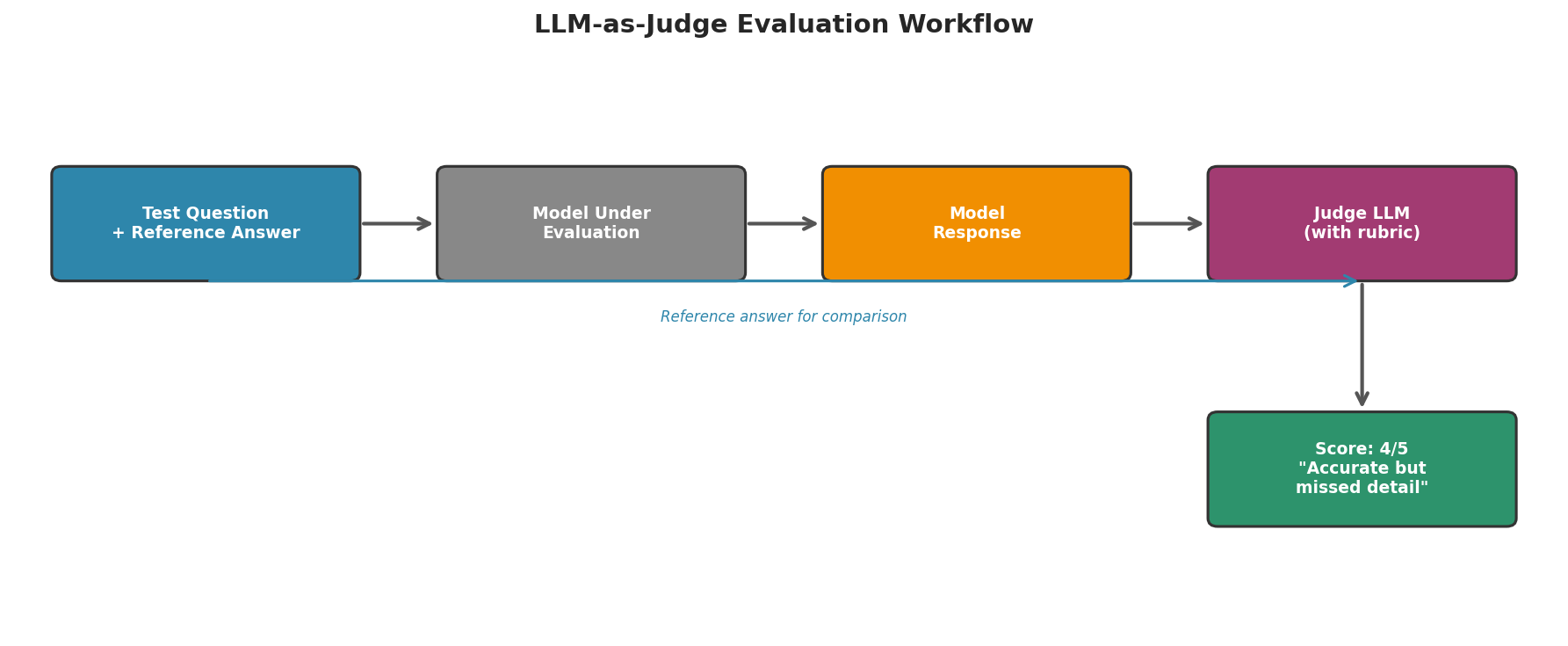
Fig. 244 Figure 6.8.3: In LLM-as-judge evaluation, a separate model evaluates the quality of the model under test. The judge receives the question, reference answer, and model response, then scores using a predefined rubric.

JUDGE_PROMPT = """You are an evaluation assistant. Score the following response
on a scale of 1-5 based on this rubric:

5: Completely accurate, well-organized, addresses all aspects
4: Mostly accurate with minor omissions
3: Partially accurate, missing important details
2: Contains significant errors or misunderstandings
1: Largely incorrect or irrelevant

### Question ###
{question}

### Reference Answer ###
{reference}

### Response to Evaluate ###
{response}

Score (1-5):"""

def judge_response(question, reference, response, ai):
    prompt = JUDGE_PROMPT.format(
        question=question, reference=reference, response=response
    )
    score_text = ai.chat(prompt).strip()
    try:
        score = int(score_text[0])
        return min(max(score, 1), 5)
    except (ValueError, IndexError):
        return 3

question = "What is the bootstrap method?"
reference = ("The bootstrap resamples observed data with replacement to "
             "estimate the sampling distribution of a statistic.")
model_response = ("The bootstrap is a statistical technique that creates "
                  "multiple datasets by randomly sampling with replacement. "
                  "It helps estimate confidence intervals.")

score = judge_response(question, reference, model_response, ai)
print(f"Judge score: {score}/5")

Judge score: 4/5

Limitations of LLM-as-Judge

LLM judges have known biases: they tend to prefer longer responses, favor responses that match their own style, and may be overly generous. Use judge scores as one signal among many, not as the sole evaluation metric.

In the SDK: a judge you can trust more

The single-judge biases above are exactly what a panel mitigates. genai_studio ships llm_judge(client, rubric=...) as a rubric-scoring judge, and critic_panel runs several independent critics with distinct models and lenses—so a lone dissenter cannot condemn a good answer and a lone booster cannot rescue a bad one. Diverse, independent judges beat a single judge for the same reason an ensemble beats a single model.

Uncertainty Quantification

Self-Consistency as Uncertainty

The self-consistency technique from Section 6.6 naturally produces an uncertainty estimate: the proportion of runs that agree with the majority answer.

from collections import Counter

def uncertainty_via_consistency(question, prompt_template, ai, n_runs=10):
    """Estimate uncertainty by measuring consistency across runs."""
    answers = [ai.chat(prompt_template.format(question=question)).strip().lower()
               for _ in range(n_runs)]
    counter = Counter(answers)
    majority, count = counter.most_common(1)[0]
    agreement = count / n_runs

    return {
        "answer": majority,
        "confidence": agreement,
        "uncertainty": 1 - agreement,
        "distribution": dict(counter),
    }

# Test on clear vs ambiguous cases
test_cases = [
    "This is the best product I have ever purchased!",
    "It works.",
    "I love the quality but hate the price.",
]

for text in test_cases:
    result = uncertainty_via_consistency(text, CLASSIFY_PROMPT, ai)
    print(f"  [{result['confidence']:.0%} conf] {result['answer']:>8} | "
          f"{text[:50]}")
    print(f"    Distribution: {result['distribution']}")

[100% conf] positive | This is the best product I have ever purchased!
  Distribution: {'positive': 10}
[70% conf]  neutral | It works.
  Distribution: {'neutral': 7, 'positive': 3}
[50% conf]  neutral | I love the quality but hate the price.
  Distribution: {'neutral': 5, 'negative': 3, 'positive': 2}

The confidence measure directly reflects the model’s stability: unambiguous inputs yield 100% agreement, while ambiguous inputs produce distributed responses. This is a natural, interpretable uncertainty measure that requires no special prompting—just multiple runs.

Bootstrap CIs on Uncertainty Estimates

The agreement rate is itself an estimate computed from a handful of runs, so it deserves the same treatment we give any estimate: an interval. Chapter 4’s bootstrap applies directly—resample the recorded answers with replacement and read off the percentiles.

import numpy as np

def bootstrap_ci_on_agreement(answers, n_bootstrap=1000, alpha=0.05):
    """Bootstrap CI on the agreement rate."""
    n = len(answers)
    counter = Counter(answers)
    majority = counter.most_common(1)[0][0]
    is_majority = np.array([1 if a == majority else 0 for a in answers])

    boot_agreements = []
    for _ in range(n_bootstrap):
        idx = np.random.choice(n, size=n, replace=True)
        boot_agreements.append(np.mean(is_majority[idx]))

    ci_low = np.percentile(boot_agreements, 100 * alpha / 2)
    ci_high = np.percentile(boot_agreements, 100 * (1 - alpha / 2))
    return ci_low, ci_high

# Get answers from multiple runs
answers = ['neutral', 'negative', 'neutral', 'neutral', 'negative',
           'neutral', 'neutral', 'negative', 'negative', 'neutral']
ci = bootstrap_ci_on_agreement(answers)
majority_rate = Counter(answers).most_common(1)[0][1] / len(answers)
print(f"Agreement: {majority_rate:.0%}")
print(f"95% Bootstrap CI: [{ci[0]:.0%}, {ci[1]:.0%}]")

Agreement: 60%
95% Bootstrap CI: [30%, 90%]

The wide CI reflects our limited sample (only 10 runs). With more runs, the CI narrows, but each run costs an API call.

Evaluation Protocols

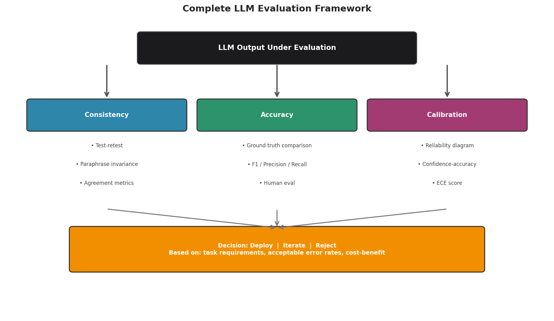
Fig. 245 Figure 6.8.4: A complete evaluation framework assesses three dimensions: consistency (does the model give stable answers?), accuracy (are the answers correct?), and uncertainty (does low agreement actually flag the wrong answers?). Together, these inform the deployment decision.

Building an Evaluation Dataset

Every protocol starts with a labeled evaluation set: a fixed collection of inputs with known answers, held apart from anything the prompt was tuned on.

def create_eval_dataset(questions, ground_truth, categories=None):
    """Create a structured evaluation dataset."""
    dataset = []
    for q, gt in zip(questions, ground_truth):
        dataset.append({
            "question": q,
            "ground_truth": gt,
            "category": categories[len(dataset)] if categories else "general",
        })
    return dataset

eval_data = create_eval_dataset(
    questions=[
        "Great product!", "Terrible quality.", "It's fine.",
        "Love everything about it!", "Worst purchase ever.",
        "Standard quality.", "Highly recommend!", "Don't buy this.",
        "Nothing special.", "Perfect in every way.",
    ],
    ground_truth=[
        "positive", "negative", "neutral",
        "positive", "negative",
        "neutral", "positive", "negative",
        "neutral", "positive",
    ],
)

Computing Evaluation Metrics

With the dataset in place, evaluation is a loop over its items: one prediction per item for accuracy and F1, several more per item to score consistency.

from sklearn.metrics import accuracy_score, f1_score

def evaluate_model(eval_data, annotate_fn, n_consistency_runs=5):
    """Complete evaluation: accuracy, F1, consistency."""
    predictions = []
    consistencies = []

    for item in eval_data:
        # Single prediction for accuracy
        pred = annotate_fn(item["question"])
        predictions.append(pred)

        # Multiple runs for consistency
        runs = [annotate_fn(item["question"]) for _ in range(n_consistency_runs)]
        agreement = Counter(runs).most_common(1)[0][1] / n_consistency_runs
        consistencies.append(agreement)

    ground_truth = [item["ground_truth"] for item in eval_data]

    acc = accuracy_score(ground_truth, predictions)
    f1 = f1_score(ground_truth, predictions, average='weighted',
                  zero_division=0)
    mean_consistency = np.mean(consistencies)

    return {
        "accuracy": acc,
        "f1_weighted": f1,
        "mean_consistency": mean_consistency,
        "predictions": predictions,
        "consistencies": consistencies,
    }

results = evaluate_model(eval_data, classify, n_consistency_runs=5)
print(f"Accuracy: {results['accuracy']:.3f}")
print(f"F1 (weighted): {results['f1_weighted']:.3f}")
print(f"Mean consistency: {results['mean_consistency']:.3f}")

Accuracy: 0.900
F1 (weighted): 0.897
Mean consistency: 0.860

In the SDK: the evaluation loop as a primitive

The consistency-and-accuracy loop we built by hand is a first-class primitive in genai_studio: from genai_studio.agents.eval import Case, evaluate runs each case k times and reports the per-run pass rate, pass@k, and self-consistency in one call—the evaluate_model / uncertainty_via_consistency pattern, packaged. Build it by hand once to understand it; reach for the primitive when you run evaluations for real.

Chapter 6.8 Exercises: Reliability and Evaluation

Exercise 6.8.1 — Consistency Audit

1. Select 15 texts (5 clearly positive, 5 clearly negative, 5 ambiguous). Run each through a sentiment classifier 10 times.

2. Compute the agreement rate for each text. Plot the distribution of agreement rates.

3. Compare the agreement rate for clear texts vs. ambiguous texts. Is the difference statistically significant? (Use a permutation test from Chapter 4.)

Solution

import numpy as np

clear_texts = [
    "Absolutely love it!", "Best ever!", "Amazing quality!",
    "Highly recommend!", "Perfect product!",
    "Terrible.", "Worst purchase.", "Complete waste.",
    "Awful quality.", "Horrible.",
]
ambiguous_texts = [
    "It's okay.", "Good but pricey.", "Not bad.",
    "Could be better.", "Mixed feelings.",
]

clear_agreements = []
for text in clear_texts:
    runs = [classify(text) for _ in range(10)]
    agreement = Counter(runs).most_common(1)[0][1] / 10
    clear_agreements.append(agreement)

ambiguous_agreements = []
for text in ambiguous_texts:
    runs = [classify(text) for _ in range(10)]
    agreement = Counter(runs).most_common(1)[0][1] / 10
    ambiguous_agreements.append(agreement)

print(f"Clear mean agreement: {np.mean(clear_agreements):.3f}")
print(f"Ambiguous mean agreement: {np.mean(ambiguous_agreements):.3f}")

# Permutation test
observed_diff = np.mean(clear_agreements) - np.mean(ambiguous_agreements)
combined = clear_agreements + ambiguous_agreements
n_clear = len(clear_agreements)
n_perm = 10000
perm_diffs = []
for _ in range(n_perm):
    perm = np.random.permutation(combined)
    d = np.mean(perm[:n_clear]) - np.mean(perm[n_clear:])
    perm_diffs.append(d)
p_value = np.mean(np.array(perm_diffs) >= observed_diff)
print(f"Permutation test p-value: {p_value:.4f}")

Exercise 6.8.2 — Does Agreement Predict Correctness?

1. Create 30 factual questions with known answers. For each, run the model 10 times (as in test_retest) and record the self-consistency agreement rate and whether the majority answer is correct—do not ask the model to rate itself.

2. Split the items into high-agreement (>= 0.8) and low-agreement (< 0.8). Compare the accuracy of each group. Is high agreement associated with higher accuracy?

3. Find the confidently wrong items—agreement >= 0.8 but the majority answer is incorrect. What fraction of high-agreement items are actually wrong? Explain why this makes the agreement rate a triage signal, not a probability of being right.

Solution

import numpy as np

questions_and_answers = [
    ("What is the capital of Japan?", "tokyo"),
    ("What is 7 * 8?", "56"),
    ("Who painted the Mona Lisa?", "leonardo"),
    # ... add 27 more
]

agree, correct = [], []
for q, truth in questions_and_answers:
    r = test_retest(q, QA_PROMPT, n_runs=10)     # 10 samples per question
    agree.append(r["agreement"])
    correct.append(int(truth.lower() in r["majority_answer"]))
agree, correct = np.array(agree), np.array(correct)

high = agree >= 0.8
print(f"high-agreement (>=0.8): accuracy {correct[high].mean():.2f}  (n={high.sum()})")
print(f"low-agreement  (<0.8):  accuracy {correct[~high].mean():.2f}  (n={(~high).sum()})")

confidently_wrong = high & (correct == 0)
print(f"confidently wrong: {confidently_wrong.sum()} of {high.sum()} high-agreement items")
# High agreement usually means higher accuracy — but the confidently-wrong
# items show it is not a guarantee, so use agreement to triage, not to trust.

Exercise 6.8.3 — LLM-as-Judge Correlation

1. Generate 10 short summaries of texts using an LLM. Manually rate each summary on a 1–5 scale (your human judgment).

2. Have an LLM judge rate the same summaries using the judge_response() function.

3. Compute the Spearman rank correlation between human and LLM judge scores. How well does the LLM judge track human preferences?

Solution

from scipy.stats import spearmanr

texts_to_summarize = [
    "Long text about bootstrap methods...",
    # ... 9 more
]

summaries = [ai.chat(f"Summarize briefly: {t}") for t in texts_to_summarize]
human_scores = [4, 3, 5, 2, 4, 3, 5, 4, 2, 3]  # Your ratings

llm_scores = []
for text, summary in zip(texts_to_summarize, summaries):
    score = judge_response(
        f"Summarize: {text[:100]}",
        text[:200],
        summary, ai
    )
    llm_scores.append(score)

rho, p_value = spearmanr(human_scores, llm_scores)
print(f"Spearman correlation: {rho:.3f} (p={p_value:.4f})")

Exercise 6.8.4 — Self-Consistency Uncertainty with Bootstrap CIs

1. Select 10 texts. For each, run 20 classification attempts and compute the majority-vote answer and agreement rate.

2. For each text, compute a 95% bootstrap CI on the agreement rate using bootstrap_ci_on_agreement().

3. Identify texts whose CI reaches 0.5 or below (the “coin flip” threshold). These are the items where the model is genuinely uncertain.

Solution

texts = [
    "Best product ever!", "Terrible quality.",
    "It's okay I guess.", "Not bad but not great.",
    "Amazing value!", "Slight disappointment.",
    "Works perfectly.", "Could be better.",
    "Love it!", "Meh.",
]

for text in texts:
    answers = [classify(text) for _ in range(20)]
    majority = Counter(answers).most_common(1)[0][0]
    agreement = Counter(answers).most_common(1)[0][1] / 20
    ci = bootstrap_ci_on_agreement(answers)
    uncertain = ci[0] <= 0.5
    print(f"  [{agreement:.0%}] CI=[{ci[0]:.0%},{ci[1]:.0%}] "
          f"{'⚠ UNCERTAIN' if uncertain else '✓'} "
          f"{majority:>8} | {text[:40]}")

Exercise 6.8.5 — Evaluation Protocol Design

Design a complete evaluation protocol for an LLM-based annotation system (e.g., the sentiment pipeline from Section 6.4). Your protocol should include:

1. An evaluation dataset (at least 30 items with ground-truth labels).

2. Metrics: accuracy, F1, Cohen’s kappa, and mean consistency.

3. A decision rule: what thresholds must be met for deployment?

4. Run the full evaluation and report results. Does the system meet your deployment criteria?

Solution

from sklearn.metrics import cohen_kappa_score

# Full evaluation protocol — each threshold is a floor the system must clear
DEPLOYMENT_CRITERIA = {
    "accuracy": 0.80,
    "f1_weighted": 0.75,
    "kappa": 0.60,
    "mean_consistency": 0.70,
}

# Create eval dataset (30+ items)
eval_dataset = create_eval_dataset(
    questions=[...],  # 30 texts
    ground_truth=[...],  # 30 ground-truth labels
)

# Run evaluation, then add Cohen's kappa (chance-corrected agreement,
# as in Section 6.4) alongside the metrics evaluate_model() reports
results = evaluate_model(eval_dataset, classify, n_consistency_runs=5)
truth = [item["ground_truth"] for item in eval_dataset]
results["kappa"] = cohen_kappa_score(truth, results["predictions"])

# Check criteria
print("Deployment Readiness Report:")
for metric, threshold in DEPLOYMENT_CRITERIA.items():
    actual = results[metric]
    passed = actual >= threshold
    status = "✓ PASS" if passed else "✗ FAIL"
    print(f"  {metric}: {actual:.3f} (threshold: {threshold}) {status}")

Transition to What Follows

Reliability assessment tells us how well an LLM performs. But there are questions beyond performance: should we use the LLM at all? Is the data safe to send to an API? Could the model’s outputs encode biases that distort our analysis? Are we obligated to disclose that AI assisted our work? In Section 6.9, we address these ethical and practical concerns—the responsible AI practices that must accompany any LLM deployment.

Key Takeaways

Key Takeaways 📝

1. LLMs are unreliable by default — hallucination, inconsistency, and overconfidence are inherent, not exceptional. Every LLM-assisted workflow needs explicit reliability checks.

2. Test-retest and paraphrase invariance measure consistency. Items with low agreement should be flagged for human review or treated with uncertainty.

3. Self-consistency is an uncertainty heuristic, not a probability. A usable confidence comes from the model’s behavior (agreement across runs), never a self-reported score—but it measures stability, not correctness: a consistently wrong model still looks sure. Validate it against ground truth and use it for triage, not as a probability of being right.

4. LLM-as-judge provides evaluation for open-ended tasks, but judge scores have known biases and should be one signal among many.

5. Self-consistency naturally produces uncertainty estimates — the agreement rate across multiple runs serves as an interpretable confidence measure, analogous to bootstrap-based inference from Chapter 4.