Appendix F: Python Random Generation
From Mathematical Distributions to Computational Samples
In Chapter 1.1, we established what probability means—whether as long-run frequencies or degrees of belief. In Appendix D, we catalogued the probability distributions that model real phenomena—Normal, Exponential, Gamma, Poisson, and dozens more—understanding their mathematical properties, relationships, and when they arise naturally.
But theoretical understanding alone doesn’t generate data. When we need 10,000 bootstrap samples, a million Monte Carlo iterations, or posterior draws from an MCMC chain, we must bridge the gap from mathematical abstraction to computational reality. This appendix provides that bridge: a comprehensive guide to Python’s ecosystem for random number generation and probability computation.
Sampling from probability distributions underpins simulation, Bayesian inference, uncertainty quantification, and generative modeling. Python offers a rich ecosystem—from the zero-dependency standard library to high-performance scientific computing frameworks. Understanding when and how to use each tool is essential for effective computational statistics.
Road Map 🧭
Understand: How pseudo-random number generators create reproducible “randomness” and why explicit seeding matters for scientific work
Develop: Fluency with Python’s
randommodule, NumPy’sGeneratorAPI, and SciPy’sstatsdistribution objectsImplement: Sampling from all distributions covered in Appendix D; weighted sampling; sequence operations
Evaluate: Performance trade-offs, parameterization conventions, and management of parallel random streams
Prerequisites Check
This appendix assumes familiarity with:
Probability distributions: families, parameters (rate vs scale), and moments (Appendix D)
Basic Python: functions, list comprehensions, and imports
The Python Ecosystem at a Glance
Before diving into details, here’s a map of the tools we’ll explore:
Category |
Library |
Why You Might Pick It |
Best For |
|---|---|---|---|
Standard Library |
|
Always available; quick scalar draws; simple shuffles; 11 classic distributions |
Teaching, prototyping, dependency-free scripts |
Scientific Computing |
|
Vectorized C/Fortran backends; roughly 5–10× faster for simple draws (more for heavier distributions); array output; 35+ distributions |
Monte Carlo, bootstrap, large-scale simulation |
Statistical Modeling |
|
100+ distributions; PDF/CDF/PPF/fitting; statistical tests |
Distribution fitting, hypothesis testing, complete statistical toolkit |
Deep Learning |
|
GPU acceleration; differentiable distributions |
Neural network initialization, VAEs, reinforcement learning |
Probabilistic Programming |
PyMC, Pyro, Stan |
High-level model syntax; MCMC & VI engines |
Complex Bayesian models (covered in Chapter 5) |
The choice of library depends on your task. As a rule of thumb:
Need just a few random numbers? →
randommoduleNeed arrays of random numbers fast? → NumPy
GeneratorNeed probability calculations (PDF, CDF, quantiles)? →
scipy.statsBuilding a Bayesian model? → PyMC, Pyro, or Stan (Chapter 5)
Understanding Pseudo-Random Number Generation
Before using any library, we should understand what’s happening under the hood. Computers are deterministic machines—given the same input, they produce the same output. So how do they generate “random” numbers? This section gives a working overview; for the full theory of how uniform generators are designed and tested, see Ch2.2.
The Nature of Pseudo-Randomness
Pseudo-random number generators (PRNGs) are deterministic algorithms that produce sequences of numbers which, while entirely predictable given the algorithm and starting point, pass stringent statistical tests for randomness. When you call random.random(), you’re executing a mathematical formula that computes the next number in a deterministic sequence.
This determinism is actually a feature, not a bug:
Reproducibility: Given the same starting point (the seed), a PRNG produces exactly the same sequence. This enables scientific reproducibility—if you report bootstrap results, others can verify your exact computation.
Debugging: When a simulation produces unexpected results, fixing the seed lets you reproduce the problematic run while investigating.
Testing: Unit tests for stochastic code can have deterministic pass/fail criteria.
What Makes a Good PRNG?
A sequence \(u_1, u_2, u_3, \ldots\) behaves like independent draws from \(\text{Uniform}(0, 1)\) if it satisfies:
Uniformity: Values should be evenly distributed across \([0, 1)\). Dividing into \(k\) equal bins, each should contain approximately \(n/k\) of \(n\) total values.
Independence: Knowing \(u_t\) should provide no information about \(u_{t+1}\). No correlation between values at any lag.
Long period: The period—the length before the sequence repeats—should vastly exceed any practical simulation length.
High-dimensional equidistribution: When consecutive outputs are used as coordinates in high-dimensional space, points should fill the space uniformly.
Modern PRNGs are tested against extensive statistical test suites (like TestU01’s BigCrush). NumPy’s default generator (PCG64) passes BigCrush; Python’s Mersenne Twister fails two of its linear-complexity tests—one motivation for preferring PCG64 in new code.
The Mersenne Twister
Python’s standard library uses the Mersenne Twister (MT19937), developed by Matsumoto and Nishimura in 1997:
Period: \(2^{19937} - 1\) (approximately \(10^{6001}\))—far exceeding any simulation need
623-dimensional equidistribution: Suitable for high-dimensional Monte Carlo
State size: 624 × 32-bit integers (19,968 bits)
Speed: Uses simple bit operations; very fast
Limitations: Not cryptographically secure (given 624 outputs, the state can be reconstructed). For security applications, use Python’s secrets module.
NumPy’s PCG64
NumPy’s modern Generator API defaults to PCG64 (Permuted Congruential Generator):
Period: \(2^{128}\) with smaller state (256 bits)
Better statistical properties: Passes even more stringent tests
Faster: Simpler operations on modern 64-bit CPUs
Jumpable: Can efficiently skip ahead, enabling parallel streams
For new projects, NumPy’s PCG64 is generally preferred over Mersenne Twister.
The Standard Library: random Module
The random module ships with every Python installation—no pip install required. It’s ideal for teaching, prototyping, and situations where external dependencies are problematic.
Generating Random Numbers
The foundation of all random generation is the uniform distribution on \([0, 1)\):
Function |
Output |
Notes |
|---|---|---|
|
|
Uniform on \([0, 1)\); the fundamental building block |
|
|
Uniform on \([a, b]\); implemented as |
|
|
Discrete uniform on \(\{a, a+1, \ldots, b\}\); inclusive on both ends |
|
|
Like |
Rule of thumb: Use random() for unit-interval floats; uniform(a, b) for self-documenting intervals; randint(a, b) for dice rolls and indices.
import random
from statistics import mean, pvariance

random.seed(42)  # For reproducibility

# Generate U(0,1) samples
n = 1000
samples = [random.random() for _ in range(n)]

# Verify distributional properties
print(f"U(0,1)  n={n}")
print(f"  mean     : {mean(samples):.5f}  (theory 0.5000)")
print(f"  variance : {pvariance(samples):.5f}  (theory 0.0833)")
print(f"  min…max  : {min(samples):.5f} … {max(samples):.5f}")
Random Operations on Sequences
Beyond generating numbers, we often need to sample from existing sequences—selecting survey respondents, shuffling experimental treatments, or drawing cards.
Function |
Returns |
Replacement? |
Size |
Weights? |
When to Use |
|---|---|---|---|---|---|
|
One element |
— |
— |
No |
Pick a single winner, coin-flip between labels |
|
List of |
With |
|
Yes |
Bootstrap resampling, Monte Carlo from categorical |
|
List of |
Without |
|
No |
Deal cards, random subset for cross-validation |
|
|
— |
whole seq |
— |
In-place permutation (e.g., shuffle deck) |
Key distinction: choices (with replacement) allows duplicates; sample (without replacement) guarantees uniqueness. Bootstrap resampling uses choices; survey sampling uses sample.
import random
from collections import Counter

random.seed(42)

# choice: single random element
volunteers = ["Alice", "Bob", "Carol", "Deepak", "Eve"]
print(f"Today's volunteer: {random.choice(volunteers)}")

# choices: weighted sampling WITH replacement (loaded die)
faces = [1, 2, 3, 4, 5, 6]
weights = [0.05, 0.10, 0.15, 0.20, 0.25, 0.25]  # Biased toward high values
rolls = random.choices(faces, weights=weights, k=10000)

print("\nLoaded die frequencies:")
for face, target_p in zip(faces, weights):
    empirical_p = rolls.count(face) / len(rolls)
    print(f"  {face}: {empirical_p:.3f}  (target {target_p:.2f})")

# sample: WITHOUT replacement (poker hand)
deck = [f"{r}{s}" for s in "♠♥♦♣" for r in "A23456789TJQK"]
hand = random.sample(deck, 5)
print(f"\nPoker hand: {hand}")

# shuffle: in-place randomization
items = list(range(10))
random.shuffle(items)
print(f"Shuffled: {items}")
Common Pitfall ⚠️
shuffle() works only on mutable sequences (lists). For strings or tuples, convert to a list first:
text = "HELLO"
letters = list(text)
random.shuffle(letters)
shuffled = ''.join(letters)  # e.g., "OELHL"
Distribution Generators
The random module provides generators for common continuous distributions. Each uses the rate or scale parameterization noted below—pay attention to avoid errors.
Function |
Distribution |
Parameters & Notes |
|---|---|---|
|
Normal \(N(\mu, \sigma^2)\) |
Slightly faster than |
|
Normal \(N(\mu, \sigma^2)\) |
Thread-safe version |
|
Exponential with rate \(\lambda\) |
Mean = \(1/\lambda\). Not scale! |
|
Gamma with shape \(\alpha\), scale \(\beta\) |
Mean = \(\alpha \beta\) |
|
Beta(\(\alpha, \beta\)) |
Support \([0, 1]\); mean = \(\alpha/(\alpha+\beta)\) |
|
Log-Normal |
\(\exp(N(\mu, \sigma^2))\) |
|
Weibull with scale \(\alpha\), shape \(\beta\) |
Note: scale first, shape second |
|
Pareto Type I with shape \(\alpha\) |
Support \([1, \infty)\) |
|
Von Mises (circular normal) |
\(\mu\) = mean angle, \(\kappa\) = concentration |
|
Triangular |
Peak at |
import random
random.seed(42)

# Normal distribution
normal_samples = [random.gauss(0, 1) for _ in range(5)]
print(f"N(0,1): {[f'{x:.3f}' for x in normal_samples]}")

# Exponential - RATE parameter (mean = 1/rate)
# For mean = 2, use rate = 0.5
exp_samples = [random.expovariate(0.5) for _ in range(5)]
print(f"Exp(rate=0.5, mean=2): {[f'{x:.3f}' for x in exp_samples]}")

# Gamma distribution
gamma_samples = [random.gammavariate(2, 3) for _ in range(5)]
print(f"Gamma(α=2, β=3): {[f'{x:.3f}' for x in gamma_samples]}")

# Beta distribution
beta_samples = [random.betavariate(2, 5) for _ in range(5)]
print(f"Beta(2,5): {[f'{x:.3f}' for x in beta_samples]}")
Example 💡: Verifying Distribution Properties
Problem: Verify that samples from standard distributions match their theoretical moments.
Implementation:
import random
from statistics import mean, pvariance
from math import gamma as math_gamma

random.seed(42)
n = 10000

distributions = [
    ("Normal(0,1)", lambda: random.gauss(0, 1), 0, 1),
    ("Exponential(λ=1)", lambda: random.expovariate(1), 1, 1),
    ("Gamma(α=2, θ=3)", lambda: random.gammavariate(2, 3), 6, 18),
    ("Beta(2,5)", lambda: random.betavariate(2, 5), 2/7, (2*5)/(49*8)),
]

print(f"{'Distribution':<22} {'Sample μ':>10} {'Theory μ':>10} {'Sample σ²':>10} {'Theory σ²':>10}")
print("-" * 66)

for name, sampler, mu_th, var_th in distributions:
    samples = [sampler() for _ in range(n)]
    mu_emp = mean(samples)
    var_emp = pvariance(samples)
    print(f"{name:<22} {mu_emp:>10.4f} {mu_th:>10.4f} {var_emp:>10.4f} {var_th:>10.4f}")
Result: Sample moments closely match theoretical values, confirming correct implementation.
Controlling Randomness: Seeds and State
Reproducibility is essential for scientific computing. The random module provides three mechanisms:
Function |
Purpose |
Key Details |
|---|---|---|
|
Initialize the PRNG |
Same seed → identical sequence; |
|
Capture full internal state |
Returns a tuple containing the 625-integer Mersenne Twister state |
|
Restore captured state |
Resumes stream exactly where it left off |
|
Independent RNG object |
Keeps multiple deterministic streams without touching global |
Typical patterns:
Scenario |
Recommended Approach |
|---|---|
Intro demo / unit test |
Call |
Pause & resume long simulation |
|
Parallel simulations |
Give each worker its own |
Temporary determinism |
Store state, run code, restore: |
import random

# Reproducibility demonstration
random.seed(42)
run1 = [random.random() for _ in range(5)]

random.seed(42)  # Reset to same seed
run2 = [random.random() for _ in range(5)]

print(f"Run 1: {run1}")
print(f"Run 2: {run2}")
print(f"Identical: {run1 == run2}")  # True

# State save/restore
random.seed(42)
_ = [random.random() for _ in range(100)]  # Advance state
saved = random.getstate()

batch1 = [random.random() for _ in range(5)]
random.setstate(saved)  # Restore
batch2 = [random.random() for _ in range(5)]
print(f"Batches match: {batch1 == batch2}")  # True
NumPy: Fast Vectorized Random Sampling
For serious scientific computing—Monte Carlo simulations, bootstrap resampling, machine learning—NumPy’s random module is essential. It’s typically 5–10× faster than Python loops for simple draws—more for heavier distributions—and provides far more distributions.
Why NumPy Is the Default for Scientific Work
Feature |
What It Buys You |
|---|---|
ndarray-native |
Draws arrive in the same structure you use for linear algebra, broadcasting, pandas I/O |
Vectorized C/Fortran core |
|
Modern Generator API |
Independent streams ( |
PCG64 PRNG |
Tiny state, period \(2^{128}\), passes BigCrush; spawns parallel streams safely |
Dozens of distributions |
Uniform to Dirichlet, plus multinomial, hypergeometric, log-series, … |
The Modern Generator API
NumPy provides two APIs: the legacy API (np.random.rand(), etc.) using global state, and the modern Generator API using explicit objects. Always use the modern API:
import numpy as np

# Create a Generator with specific seed
rng = np.random.default_rng(42)

# Generate arrays of random numbers
uniforms = rng.random(10)           # 10 U(0,1) values
normals = rng.standard_normal(10)   # 10 N(0,1) values
integers = rng.integers(1, 7, 10)   # 10 dice rolls {1,2,3,4,5,6}

print(f"Uniforms: {uniforms[:5].round(4)}")
print(f"Normals: {normals[:5].round(4)}")
print(f"Integers: {integers}")
Why explicit generators are better:
No hidden global state: Different code sections don’t interfere
Clear reproducibility: Pass generators to functions explicitly
Parallel safety: Create independent streams for workers
Better algorithms: Default PCG64 beats Mersenne Twister
Performance Comparison
import random
import numpy as np
import time

n = 1_000_000

# Python standard library
random.seed(42)
start = time.perf_counter()
python_samples = [random.random() for _ in range(n)]
python_time = time.perf_counter() - start

# NumPy Generator
rng = np.random.default_rng(42)
start = time.perf_counter()
numpy_samples = rng.random(n)
numpy_time = time.perf_counter() - start

print(f"Python: {python_time:.4f} sec")
print(f"NumPy:  {numpy_time:.4f} sec")
print(f"Speedup: {python_time/numpy_time:.1f}×")
# Typical: 5-10× speedup for simple draws; more for heavier distributions
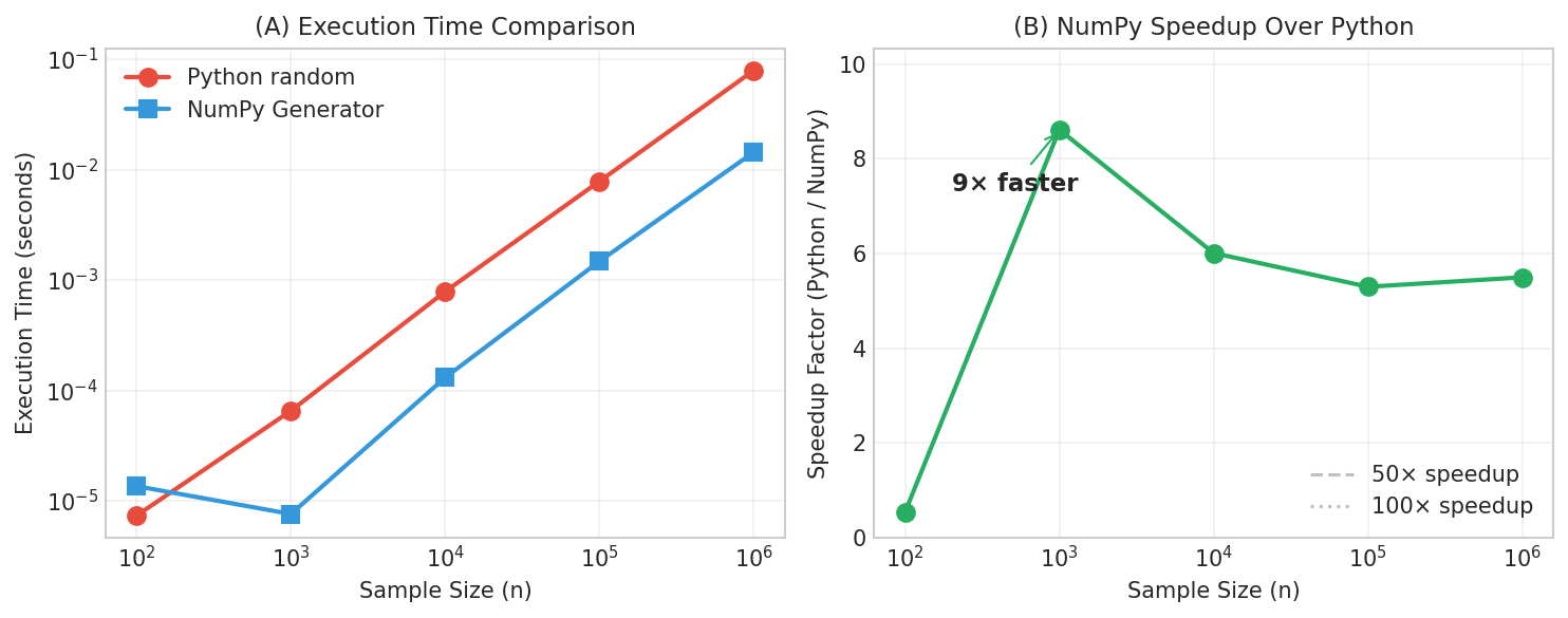
Fig. 286 NumPy Performance Advantage. Speedups of roughly 5–10× for simple draws (more for heavier distributions) come from eliminating Python’s per-element overhead, not from faster random number algorithms.
Univariate Distributions
NumPy provides generators for all distributions from Appendix D:
import numpy as np
rng = np.random.default_rng(42)
n = 10000

# Continuous distributions
uniform_01 = rng.random(n)                        # U(0,1)
uniform_ab = rng.uniform(-3, 2, n)                # U(-3, 2)
normal = rng.normal(loc=100, scale=15, size=n)   # N(100, 225)
exponential = rng.exponential(scale=2, size=n)   # Exp(scale=2), mean=2
gamma = rng.gamma(shape=2, scale=3, size=n)      # Gamma(k=2, θ=3)
beta = rng.beta(a=2, b=5, size=n)                # Beta(2, 5)

# Discrete distributions
binomial = rng.binomial(n=20, p=0.3, size=n)     # Binom(20, 0.3)
poisson = rng.poisson(lam=5, size=n)             # Poisson(λ=5)
geometric = rng.geometric(p=0.2, size=n)         # Geom(p=0.2)

# Verify moments
print(f"N(100,15²):  mean={normal.mean():.2f}, std={normal.std():.2f}")
print(f"Exp(θ=2):    mean={exponential.mean():.3f}")
print(f"Gamma(2,3):  mean={gamma.mean():.2f} (theory: 6)")
print(f"Poisson(5):  mean={poisson.mean():.2f}, var={poisson.var():.2f}")
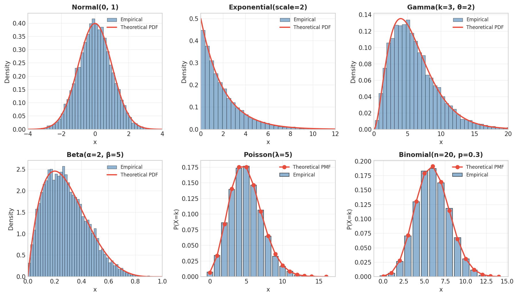
Fig. 287 Sampling from Common Distributions. Histograms of 10,000 samples with theoretical curves overlaid confirm correct implementation. The gallery uses representative parameter choices, which differ from those in the adjacent code example.
Multivariate Distributions
NumPy excels at multivariate distributions essential for modeling correlated data:
Multivariate Normal:
import numpy as np
rng = np.random.default_rng(42)

# Bivariate normal with correlation ρ = 0.8
mean = [0, 0]
cov = [[1.0, 0.8],
       [0.8, 1.0]]

samples = rng.multivariate_normal(mean, cov, size=5000)

print(f"Sample correlation: {np.corrcoef(samples.T)[0,1]:.3f}")
print(f"Sample covariance:\n{np.cov(samples.T).round(3)}")
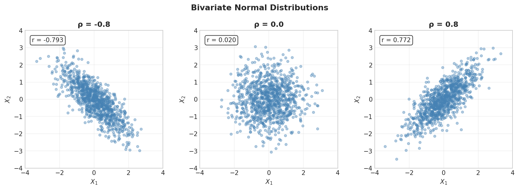
Fig. 288 Bivariate Normal with Different Correlations. Negative correlation creates downward-sloping clouds; positive correlation creates upward-sloping clouds.
Dirichlet Distribution:
The Dirichlet generates probability vectors (samples sum to 1)—essential as a prior for categorical data in Bayesian statistics:
import numpy as np
rng = np.random.default_rng(42)

# Dirichlet with concentration α = [2, 5, 3]
alpha = [2, 5, 3]
samples = rng.dirichlet(alpha, size=5)

print("Dirichlet samples (each row sums to 1):")
for i, s in enumerate(samples):
    print(f"  {i+1}: [{s[0]:.3f}, {s[1]:.3f}, {s[2]:.3f}], sum={s.sum():.6f}")

# Theoretical mean = α / sum(α)
print(f"\nTheory mean: {np.array(alpha)/sum(alpha)}")
NumPy Sampling Utilities
NumPy provides powerful functions for sampling from existing arrays:
Function |
Description |
|---|---|
|
Weighted sampling with/without replacement; axis-aware (NumPy ≥1.17) |
|
Return permuted copy along axis |
|
Shuffle in-place along axis |
|
Generate |
|
Random integers in |
import numpy as np
rng = np.random.default_rng(42)

data = np.array([10, 20, 30, 40, 50])

# Sample WITH replacement (bootstrap)
bootstrap = rng.choice(data, size=10, replace=True)
print(f"Bootstrap sample: {bootstrap}")

# Sample WITHOUT replacement
subset = rng.choice(data, size=3, replace=False)
print(f"Unique subset: {subset}")

# Weighted sampling
weights = [0.1, 0.1, 0.1, 0.3, 0.4]
weighted = rng.choice(data, size=10, replace=True, p=weights)
print(f"Weighted (favors 40,50): {weighted}")

# Axis-aware bootstrap of rows
X = np.arange(15).reshape(5, 3)
boot_rows = rng.choice(X, size=5, replace=True, axis=0)
print(f"\nOriginal:\n{X}")
print(f"Bootstrap rows:\n{boot_rows}")
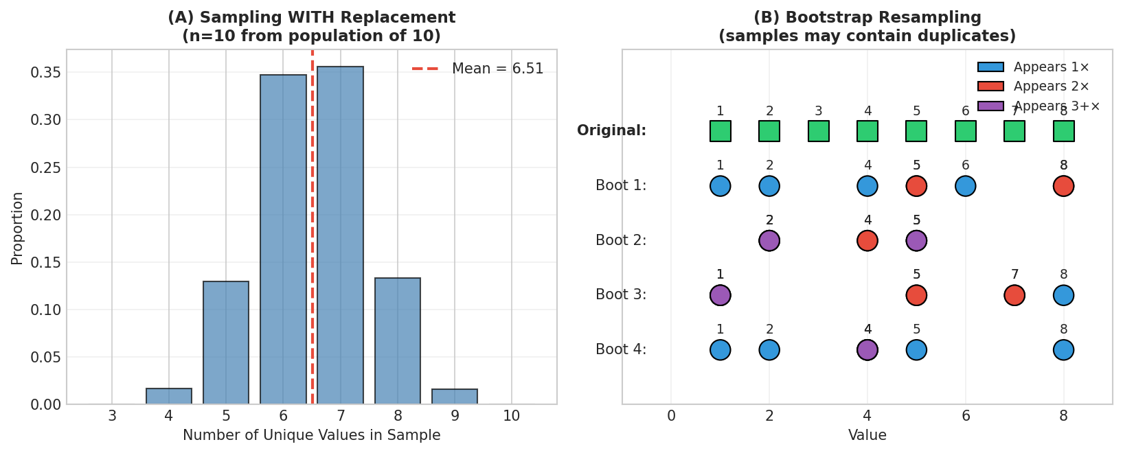
Fig. 289 Sampling With Replacement. Both panels show draws made with replacement, as in bootstrap resampling—duplicates can occur. Sampling without replacement (replace=False) would instead guarantee unique elements.
Parallel Random Number Generation
For parallel computing, each worker needs an independent random stream. Naively using seeds 0, 1, 2, … doesn’t guarantee independence. NumPy’s SeedSequence provides the solution (see Ch2.2 for the underlying theory):
import numpy as np
from numpy.random import SeedSequence, default_rng

def mc_pi(child_seed, n_points=1_000_000):
    """Estimate π using one worker's independent stream."""
    rng = default_rng(child_seed)
    x, y = rng.random(n_points), rng.random(n_points)
    return 4 * np.sum(x**2 + y**2 <= 1) / n_points

# Create master seed and spawn children
master = SeedSequence(42)
child_seeds = master.spawn(4)

# Each worker gets independent stream
estimates = [mc_pi(seed) for seed in child_seeds]
print(f"π estimates from 4 workers: {estimates}")
print(f"Mean: {np.mean(estimates):.6f}")
Common Pitfall ⚠️
Never share a Generator across threads or processes! Each parallel worker must have its own Generator from SeedSequence.spawn(). Sharing leads to:
Race conditions (undefined behavior)
Correlated streams (invalid statistics)
Non-reproducibility (results depend on timing)
SciPy Stats: The Complete Statistical Toolkit
While NumPy generates samples fast, scipy.stats provides the complete mathematical infrastructure: probability density functions, cumulative distributions, quantile functions, parameter fitting, and statistical tests.
Why SciPy Is the “Next Stop” After NumPy
Feature |
What It Buys You |
|---|---|
100+ distributions |
Gaussian to Zipf, each with PDF, CDF, PPF, RVS, fit |
Analytic functions |
Evaluate density, quantile, or survival at any point—no Monte Carlo noise |
Parameter fitting |
|
Hypothesis tests |
t-, KS-, Shapiro-Wilk, χ², Levene, Kruskal-Wallis, … |
Bootstrap helpers |
|
Decision cheat-sheet:
Task |
NumPy |
SciPy |
Go Beyond |
|---|---|---|---|
Vectorized random draws |
✅ |
— |
— |
Analytic PDF/CDF/quantile |
— |
✅ |
— |
Fit distribution parameters |
— |
✅ |
— |
Classical tests (t, KS, χ², ANOVA) |
— |
✅ |
— |
Linear/GLM/mixed models |
— |
— |
statsmodels |
Full Bayesian inference |
— |
— |
PyMC, Stan |
The Frozen Distribution Pattern
SciPy’s key design: create a distribution object with fixed parameters, then call methods on it:
from scipy import stats

# Create "frozen" distribution
iq_dist = stats.norm(loc=100, scale=15)

# Access properties
print(f"Mean: {iq_dist.mean()}")
print(f"Variance: {iq_dist.var()}")
print(f"Median: {iq_dist.median()}")

# Probability calculations
print(f"P(IQ ≤ 130) = {iq_dist.cdf(130):.4f}")
print(f"P(IQ > 130) = {iq_dist.sf(130):.4f}")

# Quantiles
print(f"90th percentile: {iq_dist.ppf(0.90):.2f}")

# Random samples
samples = iq_dist.rvs(size=5, random_state=42)
print(f"5 samples: {samples.round(1)}")
The Unified Interface
Every distribution provides the same methods:
Method |
Mathematical |
Description |
|---|---|---|
|
\(f(x)\) or \(P(X=x)\) |
Density (continuous) or mass (discrete) |
|
\(F(x) = P(X \leq x)\) |
Cumulative distribution function |
|
\(1 - F(x)\) |
Survival function |
|
\(F^{-1}(q)\) |
Quantile function (inverse CDF) |
|
— |
Random samples |
|
\(E[X]\), \(\text{Var}(X)\) |
Moments |
|
\([a,b]\): \(P(a \leq X \leq b) = \alpha\) |
Central probability interval |
|
\(\hat{\theta}_{\text{MLE}}\) |
Maximum likelihood estimation |
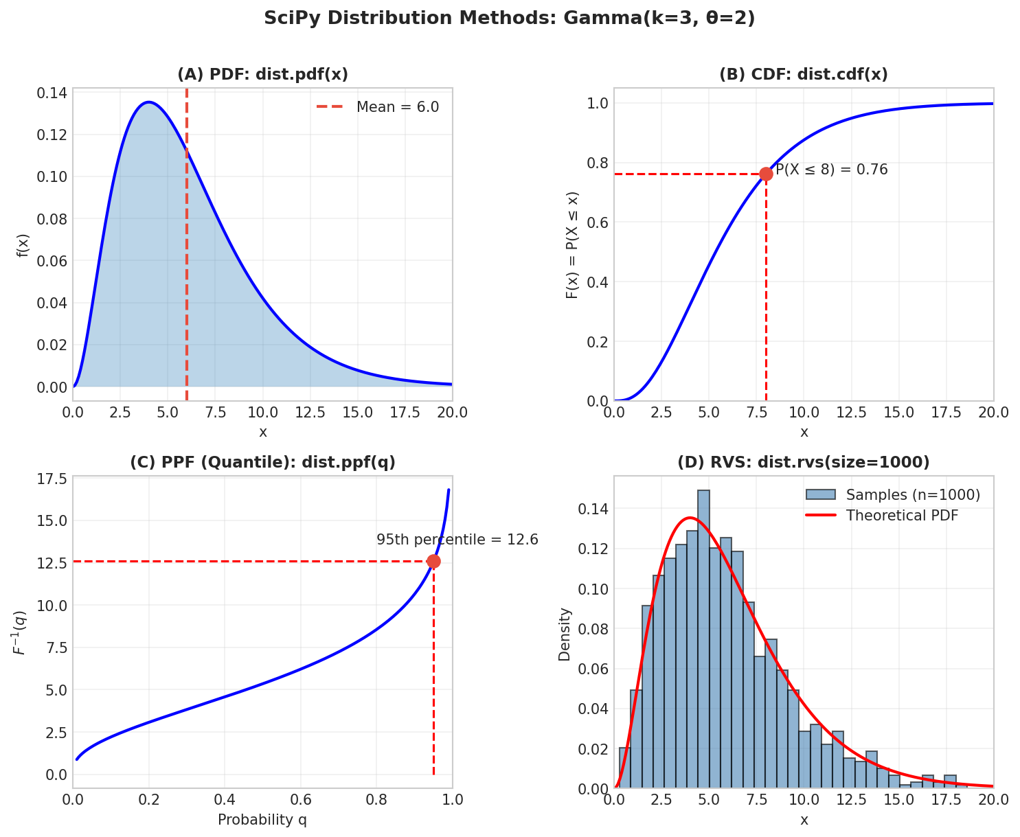
Fig. 290 SciPy Distribution Methods. (A) PDF gives density at any point. (B) CDF gives cumulative probability. (C) PPF (quantile function) inverts the CDF. (D) RVS generates samples matching the distribution.
Parameterization: The Most Common Error Source
Different sources use different parameterizations. SciPy has its own conventions:
Distribution |
SciPy Call |
Notes & Gotchas |
|---|---|---|
Normal |
|
|
Exponential |
|
Mean = scale = 1/rate. For rate λ=2, use |
Gamma |
|
|
Beta |
|
Shape parameters α, β |
Chi-square |
|
Degrees of freedom only |
Student’s t |
|
Add |
F |
|
Numerator df first |
Poisson |
|
|
Binomial |
|
n trials, probability p |
Negative Binomial |
|
Counts failures before n successes |
Common Pitfall ⚠️: Exponential Parameterization
The exponential distribution causes endless confusion:
Rate parameterization (textbooks): \(f(x) = \lambda e^{-\lambda x}\), mean = \(1/\lambda\)
Scale parameterization (SciPy/NumPy): \(f(x) = \frac{1}{\beta}e^{-x/\beta}\), mean = \(\beta\)
For mean = 2:
random.expovariate(0.5)— rate = 0.5rng.exponential(2)— scale = 2stats.expon(scale=2)— scale = 2
Always verify by checking the sample mean!
from scipy import stats
import numpy as np

# Want mean = 2
dist = stats.expon(scale=2)  # Correct
samples = dist.rvs(10000, random_state=42)
print(f"Mean: {samples.mean():.3f}")  # ≈ 2.0

# Common mistake
wrong = stats.expon(scale=0.5)  # This has mean = 0.5!
Complete Analysis Example
Example 💡: Distribution Fitting and Diagnostics
Problem: Fit a Gamma distribution to data and assess the fit.
from scipy import stats
import numpy as np

# Generate "observed" data
rng = np.random.default_rng(42)
true_dist = stats.gamma(a=2, scale=2)
data = true_dist.rvs(1000, random_state=rng)

# Fit Gamma distribution (fix location at 0)
a_hat, loc_hat, scale_hat = stats.gamma.fit(data, floc=0)
print(f"Fitted: shape={a_hat:.3f}, scale={scale_hat:.3f}")
print(f"True:   shape=2.000, scale=2.000")

# Create fitted distribution
fitted = stats.gamma(a=a_hat, loc=loc_hat, scale=scale_hat)

# Goodness-of-fit test
D, p_value = stats.kstest(data, fitted.cdf)
print(f"\nKS test: D={D:.4f}, p-value={p_value:.4f}")

# Theoretical vs empirical quantiles
print(f"\n95th percentile: fitted={fitted.ppf(0.95):.2f}, empirical={np.percentile(data, 95):.2f}")
Caveat: Because the Gamma parameters were estimated from the same data being tested, the standard KS p-value is biased toward acceptance (the Lilliefors problem); for a calibrated test, use a parametric bootstrap or a Lilliefors-type correction.
Bringing It All Together: Library Selection Guide
Use ``random`` (standard library) when:
Zero dependencies required
Teaching probability concepts
Simple prototypes or scripts
Sample sizes under ~10,000
You need
choice,shuffle,sampleon lists
Use NumPy ``Generator`` when:
Working with arrays and matrices
Sample sizes exceed 10,000
Performance is critical
You need multivariate distributions
Parallel computing with independent streams
Use ``scipy.stats`` when:
You need PDF, CDF, or quantile functions
Fitting distributions to data
Performing statistical tests
Computing theoretical properties exactly
You need exotic distributions (100+ available)
Combine them:
from scipy import stats
import numpy as np

# SciPy for distribution definition and analysis
dist = stats.gamma(a=2, scale=3)
theoretical_mean = dist.mean()
critical_value = dist.ppf(0.95)

# NumPy for efficient sampling
rng = np.random.default_rng(42)
samples = rng.gamma(shape=2, scale=3, size=100000)

# Verify
print(f"Theory mean: {theoretical_mean}, Sample mean: {samples.mean():.4f}")
Key Takeaways 📝
Pseudo-randomness is deterministic: PRNGs produce sequences determined by their seed. Reproducibility requires explicit seeding.
Three libraries, three purposes: Standard library for simplicity; NumPy for performance with arrays; SciPy for complete distribution analysis.
Know your parameterizations: Rate vs scale causes endless bugs. Always verify sample means match expectations.
Vectorize for speed: NumPy provides roughly 5–10× speedup for simple draws—more for heavier distributions—by eliminating Python loop overhead.
Independent streams for parallel work: Use
SeedSequence.spawn(). Never share generators across threads/processes.Outcome alignment: This appendix directly supports Learning Outcome 1 (simulation techniques) and provides the computational foundation for the rest of the course.
Looking Ahead: From Random Numbers to Monte Carlo Methods
With Python’s random generation ecosystem mastered, we are ready to put these tools to work. The ability to draw samples from probability distributions is not merely a computational convenience—it is the engine that powers modern statistical inference.
Chapter 2 (Ch2.1) puts these tools to work in Monte Carlo methods: using random sampling to solve problems that would be analytically intractable. The techniques you’ve learned here—generating uniforms, transforming to other distributions, managing random streams—become the building blocks for:
Monte Carlo integration: Estimating integrals via random sampling, essential when closed-form solutions don’t exist
The inverse CDF method: Transforming uniform samples to arbitrary distributions using quantile functions (
ppf)Rejection sampling: Generating samples from complex distributions by accepting/rejecting proposals
Variance reduction: Techniques like antithetic variates and control variates that improve Monte Carlo efficiency
The connection is direct: every Monte Carlo estimate begins with a call to a random number generator. The numpy.random.Generator you’ve learned to use will generate the uniform samples; the scipy.stats distributions will provide the CDFs and PDFs needed for transformations and density evaluation. Understanding the computational tools in this appendix is prerequisite to understanding why Monte Carlo methods work and how to implement them efficiently.
Consider the practice problem on parallel simulation below—it demonstrates exactly this bridge: spawning independent random streams, generating samples, and averaging to estimate a probability. Chapter 2 develops the theory behind why this works and when it fails.
Practice Problem
This exercise puts the random generation tools from this appendix into practice, focusing on the reproducibility and parallel computing patterns essential for serious simulation work.
Exercise 1: Reproducibility and Parallel Simulation
You need to run a simulation study with 4 parallel workers, each generating 25,000 samples from a mixture distribution: with probability 0.3 draw from \(N(\mu=-2, \sigma^2=1)\), otherwise draw from \(N(\mu=3, \sigma^2=0.25)\).
Background: The Parallel Reproducibility Problem
When running simulations in parallel, we need each worker to have an independent random stream, but we also want reproducibility—rerunning with the same seed should give identical results. NumPy’s SeedSequence solves this elegantly.
Implement the mixture sampler using NumPy’s
GeneratorAPI (vianp.random.default_rng()).Hint: Sampling from a Mixture
To sample from \(0.3 \cdot N(\mu_1, \sigma_1^2) + 0.7 \cdot N(\mu_2, \sigma_2^2)\):
Draw a uniform \(U \sim \text{Uniform}(0, 1)\)
If \(U < 0.3\), sample from \(N(\mu_1, \sigma_1^2)\); otherwise sample from \(N(\mu_2, \sigma_2^2)\)
Vectorized:
np.where(rng.random(size) < 0.3, rng.normal(-2, 1, size), rng.normal(3, 0.5, size))Use
SeedSequence.spawn()to create independent random streams for each worker. Verify independence by checking that the correlation between samples from different workers is near zero.Hint: SeedSequence API
from numpy.random import SeedSequence, default_rng

# Create parent seed sequence
parent_ss = SeedSequence(12345)

# Spawn independent child sequences
child_seeds = parent_ss.spawn(4)  # One per worker

# Create independent generators
rngs = [default_rng(seed) for seed in child_seeds]
Each child
SeedSequenceproduces a statistically independent stream. Verify by computingnp.corrcoef()between worker outputs—correlations should be near zero.Run the full simulation and estimate \(P(X > 0)\) along with its Monte Carlo standard error.
Hint: Monte Carlo Standard Error
If \(\hat{p} = \frac{1}{n}\sum_{i=1}^n \mathbf{1}(X_i > 0)\) is the proportion of samples exceeding 0, then:
\[\text{SE}(\hat{p}) = \sqrt{\frac{\hat{p}(1 - \hat{p})}{n}}\]Demonstrate reproducibility: re-run with the same parent seed and verify identical results.
What would go wrong if all workers shared the same
Generatorinstance? Design a small experiment to demonstrate the problem.Hint: Race Conditions
If workers share a single
Generator, the order in which they draw numbers depends on execution timing—a race condition. Different runs may produce different results even with the same seed. Demonstrate by running the same “parallel” simulation twice and showing the results differ.
Solution
Part (a): Mixture Sampler Implementation
The mixture distribution is:
Theoretical moments:
Mean: \(\mathbb{E}[X] = 0.3 \times (-2) + 0.7 \times 3 = 1.5\)
Second moment: \(\mathbb{E}[X^2] = 0.3 \times (1 + 4) + 0.7 \times (0.25 + 9) = 1.5 + 6.475 = 7.975\)
Variance: \(\text{Var}(X) = 7.975 - 1.5^2 = 5.725\)
Std: \(\sqrt{5.725} \approx 2.393\)
import numpy as np

def sample_mixture(rng, size):
    """
    Sample from mixture: 0.3 * N(μ=-2, σ=1) + 0.7 * N(μ=3, σ=0.5)

    Parameters
    ----------
    rng : np.random.Generator
        A NumPy Generator instance created via np.random.default_rng()
    size : int
        Number of samples to generate

    Returns
    -------
    np.ndarray
        Samples from the mixture distribution
    """
    # Draw component indicators: True means component 1 (N(μ=-2, σ=1))
    components = rng.random(size) < 0.3

    # Generate from both components using rng.normal(loc, scale, size)
    samples = np.where(
        components,
        rng.normal(loc=-2, scale=1, size=size),    # Component 1: N(μ=-2, σ=1)
        rng.normal(loc=3, scale=0.5, size=size)    # Component 2: N(μ=3, σ=0.5)
    )
    return samples

# Test the sampler with a reproducible Generator
rng_test = np.random.default_rng(seed=42)
test_samples = sample_mixture(rng_test, 10000)

print(f"Test run with 10,000 samples:")
print(f"  Sample mean: {np.mean(test_samples):.4f} (theoretical: 1.5000)")
print(f"  Sample std:  {np.std(test_samples):.4f} (theoretical: 2.3927)")
Test run with 10,000 samples:
  Sample mean: 1.4935 (theoretical: 1.5000)
  Sample std:  2.3977 (theoretical: 2.3927)
Part (b): Independent Random Streams
The key to parallel reproducibility is SeedSequence.spawn():
from numpy.random import SeedSequence, default_rng

parent_seed = 12345
ss = SeedSequence(parent_seed)

# Spawn 4 independent child sequences
child_seeds = ss.spawn(4)
rngs = [default_rng(s) for s in child_seeds]

# Each worker generates its samples
n_per_worker = 25000
worker_samples = [sample_mixture(rng, n_per_worker) for rng in rngs]

print(f"Parent seed: {parent_seed}")
print(f"Workers: 4, samples per worker: {n_per_worker}")

# Check independence via correlation
print(f"\nCorrelation matrix between workers:")
corr_matrix = np.corrcoef(worker_samples)
print(np.array2string(corr_matrix, precision=4, suppress_small=True))
Parent seed: 12345
Workers: 4, samples per worker: 25000

Correlation matrix between workers:
[[ 1.     -0.0046 -0.0067 -0.0105]
 [-0.0046  1.      0.0005 -0.0021]
 [-0.0067  0.0005  1.      0.0051]
 [-0.0105 -0.0021  0.0051  1.    ]]
Interpretation: Off-diagonal correlations are all within ±0.01, consistent with sampling noise for independent streams. With 25,000 samples, the expected standard error of a correlation between truly independent samples is \(1/\sqrt{n} \approx 0.006\), so these values are exactly what we’d expect.
Part (c): Estimate P(X > 0)
from scipy import stats

# Combine all samples
all_samples = np.concatenate(worker_samples)
n_total = len(all_samples)

# Monte Carlo estimate
prob_gt_0 = np.mean(all_samples > 0)
se = np.sqrt(prob_gt_0 * (1 - prob_gt_0) / n_total)

print(f"Total samples: {n_total:,}")
print(f"Estimate P(X > 0): {prob_gt_0:.4f}")
print(f"Monte Carlo SE: {se:.6f}")
print(f"95% CI: ({prob_gt_0 - 1.96*se:.4f}, {prob_gt_0 + 1.96*se:.4f})")

# Theoretical value via the mixture CDF
def mixture_cdf(x):
    return 0.3 * stats.norm.cdf(x, -2, 1) + 0.7 * stats.norm.cdf(x, 3, 0.5)

prob_theoretical = 1 - mixture_cdf(0)
print(f"\nTheoretical P(X > 0): {prob_theoretical:.4f}")
print(f"Estimation error: {abs(prob_gt_0 - prob_theoretical):.4f}")
Total samples: 100,000
Estimate P(X > 0): 0.7107
Monte Carlo SE: 0.001434
95% CI: (0.7079, 0.7135)

Theoretical P(X > 0): 0.7068
Estimation error: 0.0038
The Monte Carlo estimate is within 3 standard errors of the theoretical value—exactly the behavior we expect.

Fig. 291 Mixture Distribution and Parallel Simulation. Left: True mixture density with components shown and \(P(X > 0)\) shaded in green. Right: Histogram of 100,000 samples from 4 parallel workers matches the theoretical density closely.
Part (d): Reproducibility Demonstration
# Re-run with the same parent seed
ss_replay = SeedSequence(parent_seed)
child_seeds_replay = ss_replay.spawn(4)
rngs_replay = [default_rng(s) for s in child_seeds_replay]
worker_samples_replay = [sample_mixture(rng, n_per_worker) for rng in rngs_replay]

# Check if results are identical
identical = all(np.array_equal(a, b)
               for a, b in zip(worker_samples, worker_samples_replay))

print(f"Results identical when re-run: {identical}")
print(f"\nFirst 5 samples from worker 0:")
print(f"  Run 1: {worker_samples[0][:5]}")
print(f"  Run 2: {worker_samples_replay[0][:5]}")
Results identical when re-run: True

First 5 samples from worker 0:
  Run 1: [ 2.88863529  3.41362782 -2.45465146 -1.19442245  3.10323739]
  Run 2: [ 2.88863529  3.41362782 -2.45465146 -1.19442245  3.10323739]
Perfect reproducibility: With the same parent seed, spawn() creates identical child sequences, guaranteeing bit-for-bit identical results on the same NumPy version (NEP 19).
Part (e): Problems with Shared Generators
print("PROBLEM: Shared Generator in Parallel Execution")
print("=" * 55)

# Scenario: All workers share one generator (BAD PRACTICE)
shared_rng = np.random.default_rng(42)

# Simulate parallel execution with race conditions
# In reality, the order workers access the generator is non-deterministic

# Run 1: Worker 0, then Worker 1
run1_w0 = sample_mixture(shared_rng, 100)
run1_w1 = sample_mixture(shared_rng, 100)
run1_w0_mean = np.mean(run1_w0)

# Reset and run again
shared_rng = np.random.default_rng(42)

# Run 2: Worker 1 first (simulating different scheduling)
run2_w1 = sample_mixture(shared_rng, 100)
run2_w0 = sample_mixture(shared_rng, 100)
run2_w0_mean = np.mean(run2_w0)

print(f"\nRun 1 (W0 first): Worker 0 mean = {run1_w0_mean:.4f}")
print(f"Run 2 (W1 first): Worker 0 mean = {run2_w0_mean:.4f}")
print(f"Difference: {abs(run1_w0_mean - run2_w0_mean):.4f}")

print(f"\nWith shared generator, Worker 0 gets DIFFERENT random")
print(f"numbers depending on execution order—results are non-reproducible!")

print(f"\n" + "-" * 55)
print("SOLUTION: Independent streams (as shown in parts b-d)")
print(f"\nWith SeedSequence.spawn(), each worker gets its own")
print(f"deterministic stream, regardless of execution order.")
PROBLEM: Shared Generator in Parallel Execution
=======================================================

Run 1 (W0 first): Worker 0 mean = 1.4742
Run 2 (W1 first): Worker 0 mean = 1.7813
Difference: 0.3072

With shared generator, Worker 0 gets DIFFERENT random
numbers depending on execution order—results are non-reproducible!

-------------------------------------------------------
SOLUTION: Independent streams (as shown in parts b-d)

With SeedSequence.spawn(), each worker gets its own
deterministic stream, regardless of execution order.
Summary of problems with shared generators:
Race conditions: In true parallel execution, threads/processes may interleave their generator calls unpredictably.
Non-reproducibility: Different execution orders produce different results, even with the same seed.
Correlation artifacts: If workers happen to access the generator in a correlated pattern, their samples may inadvertently become correlated.
Performance: Lock contention on a shared generator can severely degrade parallel performance.