Section 5.3 Posterior Inference: Credible Intervals and Hypothesis Assessment
Section 5.2 built the machinery for computing posteriors — analytically for conjugate models, approximately on a grid for low-dimensional problems. But a posterior distribution is not an inferential answer; it is the raw material from which answers are extracted. This section develops the tools for extracting those answers. How do we communicate posterior uncertainty as an interval? How do we assess a directional claim such as “the treatment effect is positive”? How do we evaluate a point null hypothesis without committing to the frequentist framework of p-values and sampling distributions? And when we predict a new observation, how do we propagate both types of uncertainty that arise in any prediction: aleatoric uncertainty — the irreducible randomness in data generation that would remain even if the parameter were known exactly — and epistemic uncertainty — the uncertainty about the parameter itself, which decreases as more data are collected?
These questions have clean Bayesian answers, and the answers are often easier to interpret than their frequentist counterparts. A 95% credible interval is a probability statement about the parameter given the observed data — not a statement about the coverage of a procedure in repeated sampling. A directional probability is exactly what it sounds like: the posterior probability that the effect is in the claimed direction. These interpretations are what scientists and practitioners actually want from an interval and from a hypothesis test; the Bayesian framework delivers them directly.
The comparisons with frequentist procedures in Section 3.3 Sampling Variability and Variance Estimation will be made explicit throughout: when and how the two frameworks agree, and where they diverge in consequential ways. The methods developed here apply to any posterior — conjugate, grid-based, or MCMC — setting up the general-purpose inference tools that will be used across the remainder of the chapter.
Road Map 🧭
Understand: Why credible intervals have a more direct probabilistic interpretation than frequentist confidence intervals, and the precise conditions under which the two coincide numerically
Develop: Facility with equal-tailed credible intervals, highest density intervals, and the ROPE framework for practical hypothesis assessment
Implement: Python functions for posterior interval computation, directional probability, ROPE analysis, and posterior predictive intervals that work with any posterior representation (conjugate analytic, grid, or MCMC sample array)
Evaluate: When the choice of interval type matters, how to communicate Bayesian results to a frequentist audience, and the conditions under which Bayesian and frequentist inference yield equivalent conclusions
Credible Intervals: Probability Statements About Parameters
The fundamental difference between a Bayesian credible interval and a frequentist confidence interval is not computational — for many standard models they produce nearly identical numbers — but interpretive. Understanding this difference is not a philosophical nicety; it directly affects how results should be communicated and used.
What a Credible Interval Is
Given the posterior distribution \(p(\theta \mid y)\), a credible interval (also called a posterior interval or Bayesian interval) is a region \([L, U]\) such that:
The statement has exactly the natural interpretation: given the observed data \(y\), the probability that the parameter \(\theta\) lies in \([L, U]\) is \(1 - \alpha\). This is a probability statement about \(\theta\), which the Bayesian framework treats as a random variable with distribution \(p(\theta \mid y)\) — it is precisely because \(\theta\) is modelled as random that this probability statement is well-defined. It does not require hypothetical repetitions of the experiment; it is a statement about the current inferential state after seeing \(y\).
Contrast this with the frequentist confidence interval from Section 3.3 Sampling Variability and Variance Estimation: a 95% confidence interval is constructed by a procedure that, in 95% of hypothetical repeated experiments, will produce an interval containing the true parameter. The interval from any single experiment either contains \(\theta\) or it does not — it is not correct to say “there is a 95% probability that this particular interval contains \(\theta\).” The probability attaches to the procedure, not the realized interval.
Common Pitfall ⚠️
The most common misinterpretation in applied research is treating a frequentist 95% confidence interval as if it were a 95% credible interval — saying “there is a 95% probability that the true parameter is in this interval.” Technically this is false for the frequentist interval but true for the Bayesian credible interval. In practice, many scientists intend the Bayesian interpretation when they report frequentist intervals. The Bayesian framework delivers the interpretation they actually want, but it requires a prior. When a flat or Jeffreys prior is used and the sample is large, the two intervals are numerically similar — but the interpretation remains different, and communicating correctly matters in high-stakes applications.
Equal-Tailed Credible Intervals
Given the general credible interval definition (157), the most common construction is the equal-tailed credible interval (also called the central posterior interval), which places \(\alpha/2\) probability in each tail:
where \(\theta_q\) denotes the \(q\)-th quantile of the posterior distribution. For a posterior with closed-form quantile function (Beta, Normal, t, Gamma), computation is direct via scipy.stats:
from scipy import stats

def equal_tailed_interval(posterior_dist, level: float = 0.95) -> tuple[float, float]:
    """
    Equal-tailed credible interval from any frozen scipy distribution.

    Parameters
    ----------
    posterior_dist : scipy.stats frozen distribution
        The posterior distribution (e.g., stats.beta(40, 14)).
    level : float
        Credible interval coverage (default 0.95).

    Returns
    -------
    tuple[float, float]
        (lower, upper) interval bounds.
    """
    alpha = 1 - level
    return posterior_dist.ppf(alpha / 2), posterior_dist.ppf(1 - alpha / 2)


# Free-throw example: Curry's first 36 FT (34 makes) under a flat prior -> Beta(35, 3)
posterior = stats.beta(35, 3)
lo, hi = equal_tailed_interval(posterior)
print(f"95% ETI: ({lo:.4f}, {hi:.4f})")
print(f"Posterior mean: {posterior.mean():.4f}")
For MCMC samples or grid-based posteriors — where the posterior is represented as a weighted sample array rather than a named distribution — the equal-tailed interval is computed from the quantiles of the sample:
import numpy as np

def eti_from_samples(samples: np.ndarray,
                      level: float = 0.95) -> tuple[float, float]:
    """
    Equal-tailed credible interval from posterior samples or a
    normalized grid-weight array.

    Parameters
    ----------
    samples : np.ndarray
        1D array of posterior draws (MCMC) or grid parameter values
        with weights interpretable as a discrete posterior.
    level : float
        Coverage probability.

    Returns
    -------
    tuple[float, float]
        (lower, upper) quantile-based interval.
    """
    alpha = 1 - level
    return float(np.quantile(samples, alpha / 2)), \
           float(np.quantile(samples, 1 - alpha / 2))
Highest Density Intervals
The equal-tailed interval is not the unique \((1-\alpha)\) credible interval — any region with total posterior mass \(1-\alpha\) qualifies. Among all such regions, the Highest Density Interval (HDI) is a shortest contiguous interval (in terms of parameter-space width). For unimodal posteriors it is unique; for multimodal posteriors the globally shortest region may be a union of disjoint intervals, in which case the single-interval HDI is a useful approximation but the formally correct object is the Highest Density Region (HDR):
where \(c^*\) is chosen so that \(P(\theta \in \text{HDR}_{1-\alpha} \mid y) = 1 - \alpha\). For unimodal posteriors this set is a single interval \([L^*, U^*]\); for multimodal posteriors it is a union of intervals, each corresponding to a mode. The HDR has minimum total width — the sum of the lengths of all its component intervals — among all \((1-\alpha)\) credible regions.
Equivalently, for a unimodal posterior the HDI is the interval \([L^*, U^*]\) such that every point inside has higher posterior density than every point outside — the interval contains the most probable values of \(\theta\).
For a symmetric unimodal posterior, the ETI and HDI coincide. They diverge when the posterior is skewed. For a right-skewed posterior (common for scale parameters, rare events, or bounded quantities near their support boundary), the HDI is shifted toward the mode relative to the ETI, more accurately representing the region of highest probability mass. For multimodal posteriors, a single-interval HDI may span a low-density valley between modes — always plot the posterior before reporting any interval.
Definition: Highest Density Interval (unimodal case)
For a unimodal posterior \(p(\theta \mid y)\), the highest density interval (HDI) at level \(1-\alpha\) is the interval \([L^*, U^*]\) satisfying:
\(\int_{L^*}^{U^*} p(\theta \mid y) \, d\theta = 1 - \alpha\)
\(p(L^* \mid y) = p(U^* \mid y)\) (equal density at both endpoints — the “cutoff” condition)
For all \(\theta \in [L^*, U^*]\) and \(\theta' \notin [L^*, U^*]\): \(p(\theta \mid y) \geq p(\theta' \mid y)\)
Condition 2 defines the optimal cutoff density \(c^* = p(L^* \mid y) = p(U^* \mid y)\) such that \(\{\theta : p(\theta \mid y) \geq c^*\}\) has exactly mass \(1-\alpha\). For unimodal posteriors this level set is a single interval, and the HDI is unique up to ties at the boundary. For multimodal posteriors the level set may be a union of disjoint intervals — see the HDR implementation below.
The HDI is computed by finding the density cutoff \(c^*\) and identifying the region above it. For sample-based posteriors, a scan over sorted samples is efficient for the unimodal case; the multimodal generalisation (hdr_from_samples) uses the cutoff directly:
import numpy as np
from scipy import stats
from scipy.stats import gaussian_kde


def hdi_from_samples(samples: np.ndarray,
                      level: float = 0.95) -> tuple[float, float]:
    """
    Shortest contiguous (highest density) credible interval from
    posterior samples.  **Assumes a unimodal posterior.**

    Uses a sliding window of width = level * n_samples over the sorted
    sample array: the window with minimum width is the HDI.

    For multimodal posteriors use hdr_from_samples instead, which
    correctly returns disjoint intervals rather than a single window
    that may span a low-density valley.

    Parameters
    ----------
    samples : np.ndarray
        1D array of posterior draws.
    level : float
        Credible interval coverage (default 0.95).

    Returns
    -------
    tuple[float, float]
        (lower, upper) bounds of the HDI.
    """
    n = len(samples)
    sorted_s = np.sort(samples)
    # Width of each possible window of size floor(level * n)
    window = int(np.floor(level * n))
    widths = sorted_s[window:] - sorted_s[:n - window]
    best   = int(np.argmin(widths))
    return float(sorted_s[best]), float(sorted_s[best + window])


def hdr_from_samples(samples: np.ndarray,
                      level: float = 0.95,
                      n_grid: int = 1_000) -> list[tuple[float, float]]:
    """
    Highest Density Region (HDR) from posterior samples.

    Works for **unimodal and multimodal** posteriors.  Uses a kernel
    density estimate (KDE) — a smooth curve fitted to the sample
    histogram — to estimate the density, finds the cutoff c* such that
    the region above c* has probability mass = level, and returns the
    contiguous intervals of that region.

    Parameters
    ----------
    samples : np.ndarray
        1D array of posterior draws (MCMC or otherwise).
    level : float
        Coverage probability (default 0.95).
    n_grid : int
        Number of points for KDE evaluation (default 1_000).

    Returns
    -------
    list of tuple[float, float]
        Each tuple is (lower, upper) for one contiguous HDR segment.
        Length 1 for unimodal posteriors; length > 1 for multimodal.
    """
    kde = gaussian_kde(samples)
    theta_grid = np.linspace(samples.min(), samples.max(), n_grid)
    density    = kde(theta_grid)

    # Find c* by bisection: P(density >= c) = level
    def coverage(c):
        mask = density >= c
        # Integrate by trapezoid over the grid
        return np.trapezoid(np.where(mask, density, 0), theta_grid)

    lo_c, hi_c = 0.0, density.max()
    for _ in range(50):
        mid = (lo_c + hi_c) / 2
        if coverage(mid) > level:
            lo_c = mid
        else:
            hi_c = mid
    c_star = (lo_c + hi_c) / 2

    # Extract contiguous intervals above c*
    above = density >= c_star
    intervals = []
    in_region = False
    seg_start = None
    for i, a in enumerate(above):
        if a and not in_region:
            seg_start = theta_grid[i]
            in_region = True
        elif not a and in_region:
            intervals.append((float(seg_start), float(theta_grid[i - 1])))
            in_region = False
    if in_region:
        intervals.append((float(seg_start), float(theta_grid[-1])))

    return intervals

def hdi_from_distribution(dist,
                            level: float = 0.95,
                            n_grid: int = 10_000) -> tuple[float, float]:
    """
    HDI from a frozen scipy distribution using vectorised CDF scanning.

    Uses np.searchsorted to locate the upper bound for each candidate
    lower bound in O(N log N) time entirely in C — no Python loops.
    Safe for high-resolution grids (n_grid = 50_000+).

    Parameters
    ----------
    dist : scipy.stats frozen distribution
        Posterior (e.g., stats.beta(40, 14)).
    level : float
        Coverage probability.
    n_grid : int
        Grid resolution (default 10_000; increase for sharply peaked
        posteriors, decrease if speed is critical).

    Returns
    -------
    tuple[float, float]
        (lower, upper) HDI bounds.
    """
    lo_q, hi_q = dist.ppf(0.0001), dist.ppf(0.9999)
    theta = np.linspace(lo_q, hi_q, n_grid)
    cdf   = dist.cdf(theta)

    # For each lower-bound index i, find the smallest j such that
    # cdf[j] - cdf[i] >= level.  searchsorted locates this in O(log N)
    # per query, so the full scan is O(N log N) in C -- no Python loop.
    target_cdf   = cdf + level
    upper_indices = np.searchsorted(cdf, target_cdf)

    # Drop indices whose upper bound falls off the end of the grid
    valid      = upper_indices < n_grid
    lower_idx  = np.arange(n_grid)[valid]
    upper_idx  = upper_indices[valid]

    # Minimum-width window is the HDI
    widths   = theta[upper_idx] - theta[lower_idx]
    best     = int(np.argmin(widths))
    return float(theta[lower_idx[best]]), float(theta[upper_idx[best]])
Example 💡 ETI vs HDI for a Skewed Posterior
Given: Stephen Curry’s first 36 free throws of the 2023-24 season — 34 makes — under a flat Beta(1, 1) prior give the posterior \(\theta \mid y \sim \text{Beta}(35, 3)\). Because a make-rate is bounded above by 1, this posterior is left-skewed (mode 0.944 pressed against the upper boundary, with a long tail to the left), so the ETI and HDI will differ.
Find: The 95% ETI and HDI, and quantify the difference in interval width.
Python implementation:
import numpy as np
from scipy import stats

# Curry's first 36 free throws, 34/36, flat prior -> Beta(35, 3)
post = stats.beta(35, 3)

eti_lo, eti_hi = equal_tailed_interval(post, 0.95)
hdi_lo, hdi_hi = hdi_from_distribution(post, 0.95)

post_mode = (35 - 1) / (35 + 3 - 2)   # 0.944
print(f"Beta(35, 3): mean {post.mean():.3f}, mode {post_mode:.3f} (left-skewed)")
print(f"95% ETI: ({eti_lo:.3f}, {eti_hi:.3f})  width = {eti_hi - eti_lo:.3f}")
print(f"95% HDI: ({hdi_lo:.3f}, {hdi_hi:.3f})  width = {hdi_hi - hdi_lo:.3f}")
print(f"HDI is {(1 - (hdi_hi-hdi_lo)/(eti_hi-eti_lo))*100:.1f}% shorter than ETI")
print(f"Density at ETI ends: f(lo)={post.pdf(eti_lo):.3f}, f(hi)={post.pdf(eti_hi):.3f}")
print(f"Density at HDI ends: f(lo)={post.pdf(hdi_lo):.3f}, f(hi)={post.pdf(hdi_hi):.3f}")
Beta(35, 3): mean 0.921, mode 0.944 (left-skewed)
95% ETI: (0.818, 0.983)  width = 0.165
95% HDI: (0.836, 0.991)  width = 0.155
HDI is 6.3% shorter than ETI
Density at ETI ends: f(lo)=0.836, f(hi)=3.774
Density at HDI ends: f(lo)=1.432, f(hi)=1.431
Result: Because the posterior is left-skewed, the HDI shifts toward the mode: both of its endpoints sit higher than the ETI’s (lower bound 0.836 vs 0.818; upper bound 0.991 vs 0.983), and it is 6.3% shorter. The defining property is visible in the endpoint densities — the HDI’s two endpoints have essentially equal density (1.432 vs 1.431), whereas the ETI’s are wildly unequal (0.836 vs 3.774). The ETI spends width in the flat left tail purely to balance the two tail probabilities, even though those low values are far less plausible than the high values near 0.99 that it excludes. For a quantity bounded above — a free-throw rate, any proportion near 1, a rate near 0 — this skew is the rule rather than the exception, which is why the HDI is the more faithful “most plausible values” summary. (For a strongly skewed posterior the gap is larger still; for a symmetric posterior the two intervals coincide.)
When to Use ETI vs HDI
The choice between ETI and HDI matters primarily for asymmetric posteriors. The ETI is simpler to compute, has a direct quantile interpretation, and is analogous in structure to frequentist confidence intervals. The HDI (159) is always shorter (for unimodal distributions), always contains the posterior mode, and is the interval that most accurately represents “the most probable values.” Neither is universally superior; the choice should be based on the purpose of the interval:
ETI: preferred for symmetric posteriors, for communication with frequentist audiences (the structure is familiar), and when the interval will be used for testing procedures that require tail probabilities
HDI: preferred for skewed posteriors (scale parameters, bounded parameters), when interval length is being compared across models or studies, and when the goal is to identify the most plausible values
Property |
Equal-Tailed Interval (ETI) |
Highest Density Interval (HDI) |
|---|---|---|
Construction |
\([\theta_{\alpha/2},\, \theta_{1-\alpha/2}]\) (posterior quantiles) |
Shortest interval with mass \(1-\alpha\) |
Symmetric posteriors |
ETI = HDI |
HDI = ETI |
Skewed posteriors |
Longer; may exclude mode; “wastes” probability in thin upper tail |
Shorter; always contains mode; efficient |
Multimodal posteriors |
Single interval only; may mislead |
Single-interval HDI may span a low-density valley; use HDR ( |
Computation |
\(O(1)\) for analytic posteriors; \(O(n\log n)\) for samples |
\(O(n)\) sliding window for samples (unimodal); \(O(n)\) KDE-based HDR for multimodal |
Frequentist analog |
Closest to CI structure |
No direct analog |
Invariance to reparameterization |
Not invariant (quantiles transform non-linearly) |
Invariant under monotone increasing transforms |
Comparison with Frequentist Confidence Intervals
The numerical agreement between Bayesian credible intervals and frequentist confidence intervals under reference priors, established for specific conjugate models in Section 5.2 Prior Specification and Conjugate Analysis, generalizes as follows:
Normal model, known variance: Under a flat prior on \(\mu\), the Bayesian ETI for \(\mu\) is exactly equal to the frequentist CI: \(\bar{y} \pm z_{\alpha/2} \cdot \sigma/\sqrt{n}\).
Normal-Inverse-Gamma model: Under the reference prior, the Bayesian ETI for \(\mu\) equals the frequentist t-interval up to a one-degree-of-freedom difference (df = \(n\) vs df = \(n-1\)), which is negligible for \(n \geq 30\).
Large-sample asymptotics (Bernstein–von Mises): For any regular model and proper prior, as \(n \to \infty\) the posterior converges to a Normal distribution centered at the MLE with variance equal to the inverse Fisher information, so the Bayesian ETI and frequentist CI converge to the same interval regardless of the prior.
Small samples with informative priors: The two frameworks diverge. The Bayesian interval reflects both the data and the prior; the frequentist interval reflects only the data. Which is more appropriate depends on whether the prior information is scientifically defensible.
The key asymmetry: when a frequentist confidence interval contains a boundary value (e.g., zero, or the boundary of a bounded parameter space), it can produce nonsensical intervals — confidence intervals for a proportion that extend below 0 or above 1, for instance. Bayesian credible intervals derived from posteriors supported on \([0,1]\) are naturally constrained to the support; they cannot exceed the boundary.
Posterior Probability and Directional Hypothesis Assessment
In the frequentist framework, hypothesis testing begins with a null hypothesis and asks: if the null were true, how likely is the observed data or something more extreme? The resulting p-value does not answer the question scientists most often want to ask: given the observed data, how probable is the hypothesis?
The Bayesian framework answers this question directly. Given the posterior \(p(\theta \mid y)\), the probability that \(\theta\) exceeds any threshold \(\theta_0\) is simply:
where \(F_{\text{post}}\) is the posterior CDF. This is a genuine probability, not a tail-area under a null distribution.
Directional Probabilities
The most common application is assessing whether an effect is positive:
import numpy as np
from scipy import stats


def posterior_probability(posterior_dist,
                            threshold: float = 0.0,
                            direction: str = 'greater') -> float:
    """
    Compute the posterior probability that the parameter exceeds
    (or falls below) a threshold.

    Parameters
    ----------
    posterior_dist : scipy.stats frozen distribution
        Posterior distribution.
    threshold : float
        The threshold value theta_0.
    direction : str
        'greater' for P(theta > threshold | y),
        'less'    for P(theta < threshold | y).

    Returns
    -------
    float
        Posterior probability in [0, 1].
    """
    if direction == 'greater':
        return float(1 - posterior_dist.cdf(threshold))
    elif direction == 'less':
        return float(posterior_dist.cdf(threshold))
    else:
        raise ValueError("direction must be 'greater' or 'less'")


def posterior_probability_from_samples(samples: np.ndarray,
                                        threshold: float = 0.0,
                                        direction: str = 'greater') -> float:
    """
    Compute directional posterior probability from sample array.

    Works for any posterior representation (MCMC, grid-weighted samples).

    Parameters
    ----------
    samples : np.ndarray
        1D array of posterior draws.
    threshold : float
        The threshold value.
    direction : str
        'greater' or 'less'.

    Returns
    -------
    float
        Estimated posterior probability.
    """
    if direction == 'greater':
        return float(np.mean(samples > threshold))
    elif direction == 'less':
        return float(np.mean(samples < threshold))
    else:
        raise ValueError("direction must be 'greater' or 'less'")
Example 💡 Directional Assessment — Is Curry Truly Elite?
Given: Curry’s early free-throw posterior Beta(35, 3) (34 makes in his first 36 attempts, flat prior). Two natural thresholds: the league free-throw rate is about 0.78, and an “elite” shooter is conventionally one who makes 90% or more.
Find:
\(P(\theta > 0.90 \mid y)\) — posterior probability that Curry’s true rate is elite (90%+)
\(P(\theta > 0.78 \mid y)\) — posterior probability that he is above league average
Compare with one-sided frequentist p-values for the same hypotheses
Python implementation:
import numpy as np
from scipy import stats

# Flat prior: Beta(1,1) + 34 makes in 36 attempts → Beta(35, 3)
posterior = stats.beta(35, 3)
k, n = 34, 36

# (a) elite (90%+) and (b) above league average (78%)
p_elite        = posterior_probability(posterior, 0.90, 'greater')
p_above_league = posterior_probability(posterior, 0.78, 'greater')

# (c) Frequentist one-sided p-values: P(K >= 34 | theta = theta_0, n=36)
p_freq_090 = 1 - stats.binom.cdf(k - 1, n, 0.90)
p_freq_078 = 1 - stats.binom.cdf(k - 1, n, 0.78)

print(f"Posterior Beta(35, 3):  mean={posterior.mean():.4f}, "
      f"mode={(35-1)/(35+3-2):.4f}")
print()
print("Bayesian directional probabilities:")
print(f"  P(theta > 0.90 | y) = {p_elite:.4f}"
      f"  [{p_elite*100:.1f}%]   (truly elite?)")
print(f"  P(theta > 0.78 | y) = {p_above_league:.4f}"
      f"  [{p_above_league*100:.1f}%]   (above league average?)")
print()
print("Frequentist one-sided p-values:")
print(f"  p-value (H0: theta=0.90) = {p_freq_090:.4f}")
print(f"  p-value (H0: theta=0.78) = {p_freq_078:.4f}")

# Posterior probability breakdown
rng = np.random.default_rng(42)
samples = rng.beta(35, 3, size=100_000)
print()
print("Monte Carlo verification (100k samples):")
print(f"  P(theta > 0.90) = {(samples > 0.90).mean():.4f}")
print(f"  P(theta > 0.78) = {(samples > 0.78).mean():.4f}")
Posterior Beta(35, 3):  mean=0.9211, mode=0.9444

Bayesian directional probabilities:
  P(theta > 0.90 | y) = 0.7297  [73.0%]   (truly elite?)
  P(theta > 0.78 | y) = 0.9934  [99.3%]   (above league average?)

Frequentist one-sided p-values:
  p-value (H0: theta=0.90) = 0.2879
  p-value (H0: theta=0.78) = 0.0080

Monte Carlo verification (100k samples):
  P(theta > 0.90) = 0.7295
  P(theta > 0.78) = 0.9937
Result: The posterior answers each question directly: it is near-certain (99.3%) that Curry is above league average, but only moderately likely (73.0%) that his true rate clears the elite 90% bar — 36 attempts are simply not enough to settle the second claim. The frequentist p-values address the different “how surprising under the null” question: \(p = 0.008\) rejects \(\theta = 0.78\) at the 5% level, while \(p = 0.288\) cannot reject \(\theta = 0.90\) — but neither p-value reports the probability of the claim itself, which is what an analyst actually wants. This is also where directional probability and a point estimate diverge: the MLE (0.944) sits comfortably above 0.90, yet the posterior puts only 73% of its mass there.
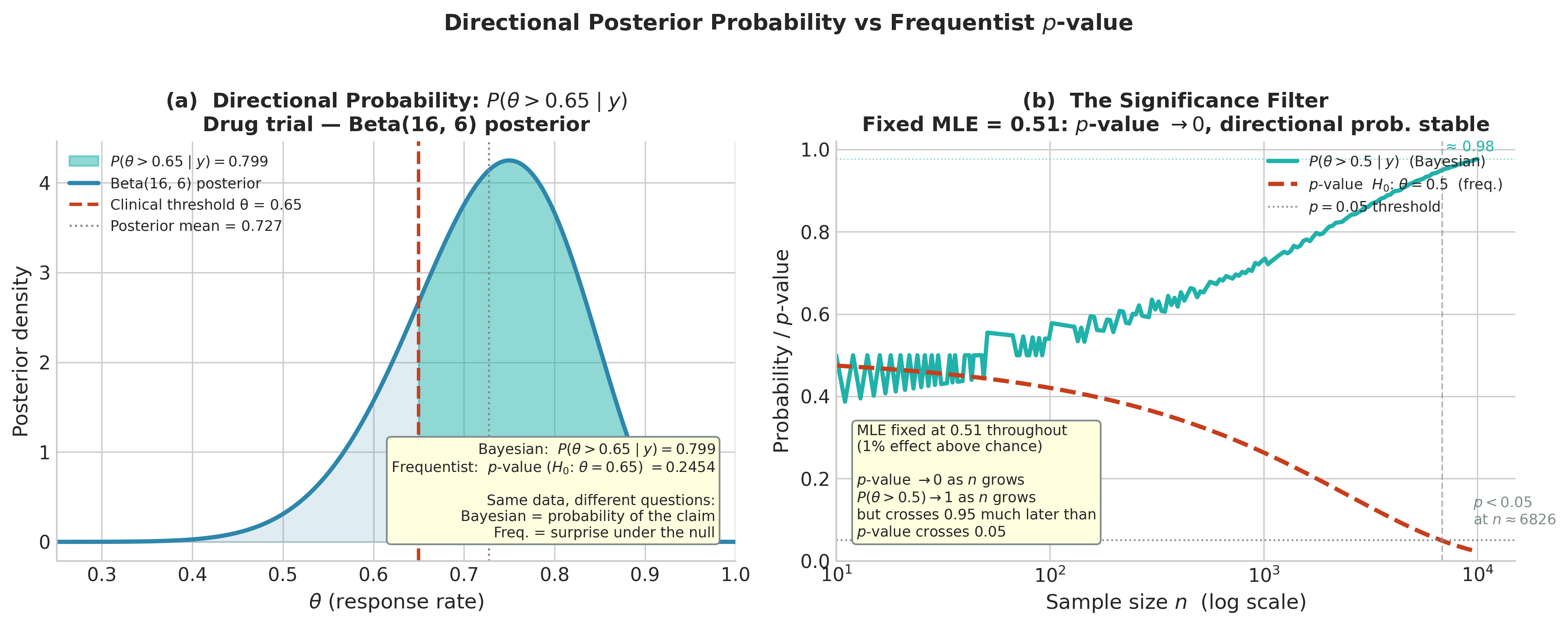
Fig. 188 Figure 5.17: Directional posterior probability vs. frequentist p-value. Left: Curry’s Beta(35, 3) posterior with the “elite” region \(\theta > 0.90\) shaded; the posterior probability of that claim (73.0%) is read directly from the shaded area, while the frequentist p-value (0.288) answers the different question of how surprising 34 makes in 36 would be if \(\theta = 0.90\) exactly. Right: the significance filter — for a shooter genuinely 1 percentage point above league average (MLE fixed at 0.79, null 0.78), both \(P(\theta > 0.78 \mid y)\) and the p-value evolve as \(n\) grows. The p-value crosses 0.05 at a moderate sample size, declaring “statistical significance” for a practically negligible one-point edge, while the Bayesian directional probability climbs toward 1 without the binary threshold. The ROPE analysis below is the appropriate tool for assessing practical significance.
Region of Practical Equivalence (ROPE)
Point null hypotheses — \(H_0: \theta = \theta_0\) — rarely make scientific sense. An effect size of exactly zero is physically implausible in most applications; the interesting question is whether the effect is large enough to matter. The Region of Practical Equivalence (ROPE) framework, introduced by Kruschke (2011), operationalizes this by defining a small interval around the null value:
where \(\epsilon\) is chosen based on domain knowledge — the smallest effect size that would be scientifically or practically meaningful. The analysis then examines the relationship between the posterior and the ROPE:
Definition: ROPE Decision Rules
Given a posterior \(p(\theta \mid y)\) and a ROPE \([\theta_0 - \epsilon, \theta_0 + \epsilon]\):
Accept :math:`H_0` (declare practical equivalence): if the 95% HDI lies entirely inside the ROPE
Reject :math:`H_0` (declare practical significance): if the 95% HDI lies entirely outside the ROPE
Remain undecided: if the HDI overlaps the ROPE — more data are needed
The posterior probability in the ROPE is a continuous summary of evidence:
This framework avoids the binary accept/reject structure of null hypothesis testing while still providing operational decision criteria. The decision depends on both the posterior and the ROPE (161), both of which are substantively specified.
import numpy as np
from scipy import stats
from dataclasses import dataclass


@dataclass
class ROPEResult:
    """
    Summary of a ROPE analysis.

    Attributes
    ----------
    p_rope : float
        Posterior probability inside the ROPE.
    p_below : float
        Posterior probability below ROPE (effect negative).
    p_above : float
        Posterior probability above ROPE (effect positive).
    hdi_lo, hdi_hi : float
        95% HDI bounds.
    decision : str
        'accept H0', 'reject H0', or 'undecided'.
    """
    p_rope:    float
    p_below:   float
    p_above:   float
    hdi_lo:    float
    hdi_hi:    float
    rope_lo:   float
    rope_hi:   float
    decision:  str

    def __str__(self) -> str:
        return (f"ROPE [{self.rope_lo:.3f}, {self.rope_hi:.3f}]\n"
                f"  P(in ROPE)   = {self.p_rope:.4f}\n"
                f"  P(below)     = {self.p_below:.4f}\n"
                f"  P(above)     = {self.p_above:.4f}\n"
                f"  95% HDI      = ({self.hdi_lo:.4f}, {self.hdi_hi:.4f})\n"
                f"  Decision     = {self.decision}")


def rope_analysis(posterior_dist,
                   rope_lo: float,
                   rope_hi: float,
                   level: float = 0.95) -> ROPEResult:
    """
    ROPE analysis from a frozen scipy posterior distribution.

    Parameters
    ----------
    posterior_dist : scipy.stats frozen distribution
        The posterior.
    rope_lo, rope_hi : float
        Lower and upper ROPE bounds.
    level : float
        HDI coverage (default 0.95).

    Returns
    -------
    ROPEResult
        Structured summary with probabilities and decision.
    """
    p_rope  = float(posterior_dist.cdf(rope_hi) - posterior_dist.cdf(rope_lo))
    p_below = float(posterior_dist.cdf(rope_lo))
    p_above = float(1 - posterior_dist.cdf(rope_hi))
    h_lo, h_hi = hdi_from_distribution(posterior_dist, level)

    # Decision rules
    if h_hi <= rope_hi and h_lo >= rope_lo:
        decision = 'accept H0 (HDI inside ROPE)'
    elif h_lo >= rope_hi or h_hi <= rope_lo:
        decision = 'reject H0 (HDI outside ROPE)'
    else:
        decision = 'undecided (HDI overlaps ROPE)'

    return ROPEResult(p_rope, p_below, p_above, h_lo, h_hi,
                       rope_lo, rope_hi, decision)
Example 💡 ROPE Analysis — Clinical Equivalence
Given: Three real shooters, each asked the same question — is this player’s true free-throw rate practically league-average? The league rate is about 0.78, so we treat rates within ±0.02 of it as practically equivalent to average: ROPE = [0.76, 0.80].
Holiday: first 31 free throws, \(k=26\) (flat prior → Beta(27, 6)) — a small sample
Westbrook: career 6109 of 7928 (flat prior → Beta(6110, 1820)) — a genuine ~0.77 career shooter
Curry: full 2023-24 season, 299 of 324 (flat prior → Beta(300, 26)) — elite
Find: For each shooter, the posterior probability in the ROPE and the ROPE decision.
Python implementation:
import numpy as np
from scipy import stats

shooters = [
    ('Holiday (first 31 FTA)',       stats.beta(27,   6)),
    ('Westbrook (career 6109/7928)', stats.beta(6110, 1820)),
    ('Curry (full season 299/324)',  stats.beta(300,  26)),
]
rope_lo, rope_hi = 0.76, 0.80   # "practically league-average" (0.78 ± 0.02)

for name, posterior in shooters:
    result = rope_analysis(posterior, rope_lo, rope_hi)
    print(f"\n{name}:")
    print(result)
Holiday (first 31 FTA):
ROPE [0.760, 0.800]
  P(in ROPE)   = 0.1750
  P(below)     = 0.1852
  P(above)     = 0.6398
  95% HDI      = (0.6873, 0.9381)
  Decision     = undecided (HDI overlaps ROPE)

Westbrook (career 6109/7928):
ROPE [0.760, 0.800]
  P(in ROPE)   = 0.9862
  P(below)     = 0.0138
  P(above)     = 0.0000
  95% HDI      = (0.7606, 0.7801)
  Decision     = accept H0 (HDI inside ROPE)

Curry (full season 299/324):
ROPE [0.760, 0.800]
  P(in ROPE)   = 0.0000
  P(below)     = 0.0000
  P(above)     = 1.0000
  95% HDI      = (0.8898, 0.9486)
  Decision     = reject H0 (HDI outside ROPE)
Result: The three shooters realise the three different ROPE verdicts. Holiday’s 31 attempts leave the posterior too diffuse — its HDI (0.687–0.938) straddles the ROPE, so the honest verdict is undecided: we cannot yet say whether he is league-average. Westbrook, with nearly 8,000 career attempts, has a posterior so tight (HDI 0.761–0.780) that it sits entirely inside the ROPE — we accept practical equivalence; he is, to high precision, a genuinely league-average free-throw shooter. Curry’s full season concentrates his HDI (0.890–0.949) entirely above the ROPE — we reject practical equivalence and conclude his rate is meaningfully better than average. Note that “accept” here is a real, data-earned conclusion (Westbrook’s enormous sample buys it), not the frequentist’s “fail to reject.”
![Three-panel ROPE cascade showing Beta(27,6) (Holiday), Beta(6110,1820) (Westbrook), and Beta(300,26) (Curry) posteriors with the ROPE [0.76,0.80] shaded in amber and the 95% HDI annotated in each panel; the decision badge reads undecided (Holiday), accept H0 (Westbrook), and reject H0 (Curry).](https://pqyjaywwccbnqpwgeiuv.supabase.co/storage/v1/object/public/STAT%20418%20Images/assets/PartIII/Chapter5/ch5_3_fig18_rope_cascade.png)
Fig. 189 Figure 5.18: ROPE analysis across three real free-throw shooters against the “practically league-average” region \([0.76, 0.80]\) (league rate ≈ 0.78 ± 0.02). Left (Holiday, first 31 FTA, Beta(27, 6)): the small sample leaves a wide HDI (0.687–0.938) straddling the ROPE — undecided. Center (Westbrook, career 6109/7928, Beta(6110, 1820)): nearly 8,000 attempts pin the HDI (0.761–0.780) entirely inside the ROPE — accept practical equivalence, a genuine league-average shooter. Right (Curry, full season 299/324, Beta(300, 26)): the HDI (0.890–0.949) lies entirely above the ROPE — reject practical equivalence; Curry is meaningfully better than average. The three shooters realise the three ROPE outcomes — undecided, accept, reject — driven by sample size and true rate rather than by a binary threshold.
Try It Yourself 🖥️
The ROPE & HDI Decision Dashboard makes the three-outcome decision rule dynamic. Drag the sample size \(n\) from 4 to 300 and watch the HDI shrink until it crosses the ROPE boundary, flipping the decision from “undecided” to “reject” in real time.
Launch: ROPE & HDI Decision Dashboard
Experiments to try:
Reproduce the three outcomes: Set ROPE centre = 0.78, ε = 0.02 (“practically league-average”). A small high-rate sample (e.g. \(k/n \approx 0.84\), \(n = 31\)) stays undecided; a large league-average sample (\(k/n \approx 0.77\), large \(n\)) is accepted; an elite rate (\(k/n \approx 0.92\)) is rejected.
Effect of ROPE width: Fix \(n = 50\) and widen ε from 0.05 to 0.25. How much does the ROPE need to widen before “undecided” flips to “accept H₀”?
Prior influence: Increase α₀ from 1 to 10 (a strongly informative symmetric prior). At fixed \(n = 20\), does the prior shrink or widen the HDI? In which direction does it pull the decision?
Keyboard shortcut: ← / → adjust \(n\) in steps of 5 without touching the slider.
Posterior Predictive Intervals
A posterior predictive interval quantifies uncertainty about a future observation \(\tilde{y}\) and is generally wider, because it incorporates both:
Epistemic uncertainty: uncertainty about \(\theta\), captured by the posterior width
Aleatoric uncertainty: inherent sampling variability, \(p(\tilde{y} \mid \theta)\)
The posterior predictive distribution, derived in Section 5.1 Foundations of Bayesian Inference, is:
This marginalizes over all possible values of \(\theta\), weighted by their posterior probability, as defined in (162). For conjugate models, the posterior predictive often has a closed form (Beta-Binomial for binary outcomes, Negative Binomial for count outcomes, t-distribution for Normal observations). For non-conjugate models, it is approximated by Monte Carlo:
Frequentist prediction intervals, by contrast, condition on a single point estimate \(\hat{\theta}\) and add an additional term for estimation uncertainty via the delta method or bootstrap. The Bayesian predictive is the natural, internally consistent approach that propagates all uncertainty automatically.
Computational Framework
The following utility function generates posterior predictive samples from any model and supports both analytic and sample-based posteriors:
import numpy as np
from scipy import stats


def posterior_predictive_interval(
    posterior_dist,
    likelihood_sampler,
    n_new: int = 1,
    level: float = 0.95,
    n_mc: int = 50_000,
    rng: np.random.Generator | None = None,
    interval_type: str = 'eti'
) -> tuple[float, float]:
    """
    Posterior predictive interval by Monte Carlo integration.

    Samples theta from the posterior, then samples new observations
    from the likelihood — propagating both epistemic and aleatoric
    uncertainty into the interval.

    Parameters
    ----------
    posterior_dist : scipy.stats frozen distribution
        Posterior distribution for the parameter(s).
    likelihood_sampler : callable
        Signature (theta_samples, rng, n_new) -> array of shape
        (n_mc, n_new). Generates new observations from the likelihood
        given posterior draws.
    n_new : int
        Number of new observations to predict (default 1).
    level : float
        Predictive interval coverage (default 0.95).
    n_mc : int
        Number of Monte Carlo samples.
    rng : np.random.Generator, optional
        For reproducibility.
    interval_type : str
        'eti' for equal-tailed, 'hdi' for highest density.

    Returns
    -------
    tuple[float, float]
        (lower, upper) posterior predictive interval bounds.
    """
    if rng is None:
        rng = np.random.default_rng()

    # Step 1: draw from posterior
    theta_samples = posterior_dist.rvs(size=n_mc, random_state=rng)

    # Step 2: draw new observations given each posterior draw
    y_new = likelihood_sampler(theta_samples, rng, n_new)

    # Step 3: compute interval from the predictive sample
    y_flat = y_new.ravel() if n_new == 1 else y_new.mean(axis=1)
    if interval_type == 'eti':
        return eti_from_samples(y_flat, level)
    else:
        return hdi_from_samples(y_flat, level)
Example 💡 Comparing Credible and Predictive Intervals
Given: Curry’s early free-throw posterior Beta(35, 3). We want to compare:
The 95% credible interval for the true make rate \(\theta\)
The 95% posterior predictive interval for the number of makes in his next 20 free throws
A 95% frequentist prediction interval using the plug-in estimate
Mathematical approach:
For the Beta-Binomial predictive, the exact distribution for \(\tilde{k}\) new successes in \(m = 20\) trials is:
Python implementation:
import numpy as np
from scipy import stats
from scipy.special import gammaln, betaln

rng = np.random.default_rng(42)
posterior = stats.beta(35, 3)
m_new = 20

# (a) 95% credible interval for theta
cri_lo, cri_hi = equal_tailed_interval(posterior)
print(f"(a) 95% Credible Interval for theta: ({cri_lo:.4f}, {cri_hi:.4f})")
print(f"    Width: {cri_hi - cri_lo:.4f}")

# (b) Posterior predictive: Beta-Binomial distribution
def beta_binomial_pmf(k, m, a, b):
    log_pmf = (gammaln(m+1) - gammaln(k+1) - gammaln(m-k+1)
               + gammaln(k+a) + gammaln(m-k+b) - gammaln(m+a+b)
               + gammaln(a+b) - gammaln(a) - gammaln(b))
    return np.exp(log_pmf)

k_vals = np.arange(0, m_new + 1)
pred_pmf = beta_binomial_pmf(k_vals, m_new, 35, 3)
pred_cdf = np.cumsum(pred_pmf)

pred_lo = int(k_vals[np.argmax(pred_cdf >= 0.025)])
pred_hi = int(k_vals[np.argmax(pred_cdf >= 0.975)])
pred_mean = np.sum(k_vals * pred_pmf)
pred_var  = np.sum(k_vals**2 * pred_pmf) - pred_mean**2

print(f"\n(b) 95% Posterior Predictive Interval for k_new in {m_new} free throws:")
print(f"    [{pred_lo}, {pred_hi}]  ({pred_lo/m_new:.2f} to {pred_hi/m_new:.2f})")
print(f"    Predictive mean: {pred_mean:.3f}  std: {pred_var**0.5:.3f}")

# (c) Plug-in prediction: Binomial with theta = MLE
mle = 34 / 36
binom_dist = stats.binom(m_new, mle)
plug_lo = int(binom_dist.ppf(0.025))
plug_hi = int(binom_dist.ppf(0.975))
print(f"\n(c) Frequentist Plug-in Prediction Interval for k_new:")
print(f"    [{plug_lo}, {plug_hi}]  ({plug_lo/m_new:.2f} to {plug_hi/m_new:.2f})")
print(f"    (ignores estimation uncertainty in theta; std: {binom_dist.std():.3f})")
(a) 95% Credible Interval for theta: (0.8180, 0.9831)
    Width: 0.1651

(b) 95% Posterior Predictive Interval for k_new in 20 free throws:
    [15, 20]  (0.75 to 1.00)
    Predictive mean: 18.421  std: 1.471

(c) Frequentist Plug-in Prediction Interval for k_new:
    [17, 20]  (0.85 to 1.00)
    (ignores estimation uncertainty in theta; std: 1.024)
Result: The posterior predictive interval [15, 20] is wider than the plug-in interval [17, 20] and reaches further into the lower tail. The predictive interval is wider because the Bayesian prediction accounts for uncertainty in \(\theta\) — some posterior mass sits on smaller make rates, which generate fewer makes — whereas the plug-in interval uses \(\hat{\theta} = 0.944\) as if it were known exactly, placing too little probability on low-count outcomes. The predictive standard deviation (1.47) exceeds the plug-in Binomial standard deviation (1.02), quantifying the additional uncertainty from not knowing \(\theta\). The credible interval in (a) answers “where is Curry’s true rate?”; the predictive interval in (b) answers “how many of his next 20 will he make?” — different questions, not interchangeable.
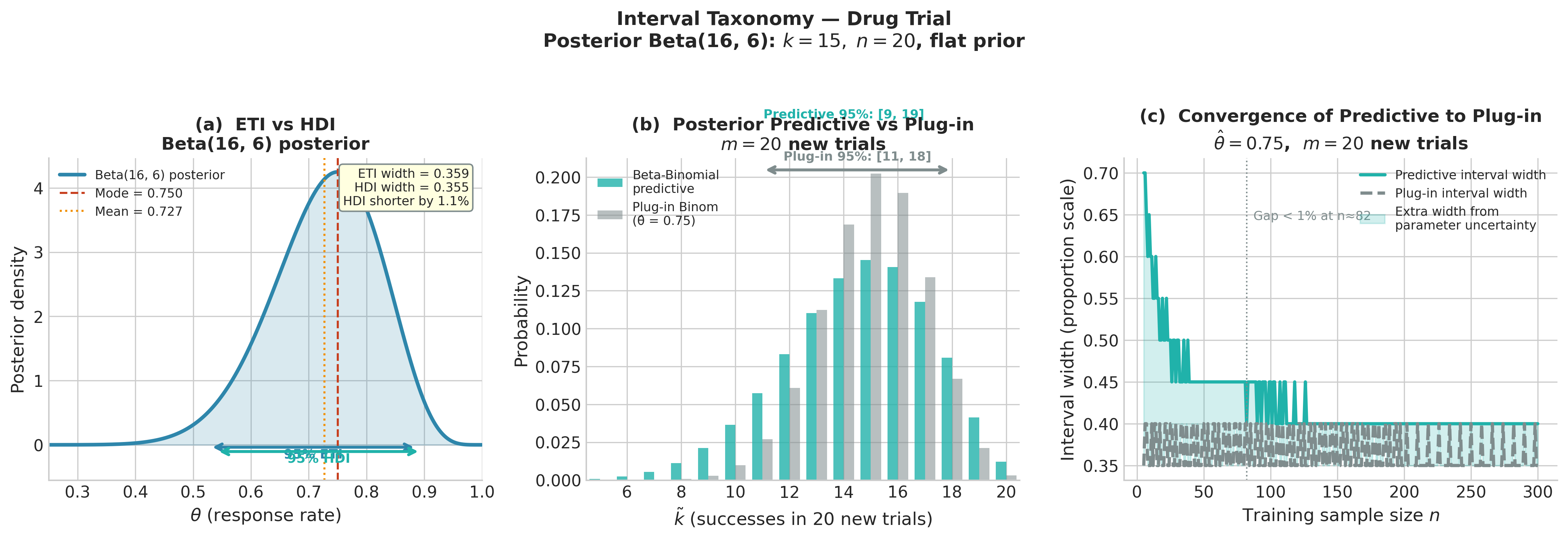
Fig. 190 Figure 5.19: Interval taxonomy for Curry’s free throws. Left: the posterior Beta(35, 3) with the 95% ETI (blue bracket, width 0.165) and HDI (teal bracket, width 0.155); because the posterior is left-skewed the HDI shifts toward the mode (0.944) and is 6.3% shorter. Center: the Beta-Binomial posterior predictive PMF for the next 20 free throws (teal bars) vs. the plug-in Binomial at \(\hat{\theta} = 0.944\) (grey bars); the 95% predictive interval [15, 20] is wider and reaches lower than the plug-in interval [17, 20] because the predictive marginalizes over uncertainty in \(\theta\), assigning more probability to lower-count outcomes. Right: interval width as a function of training sample size \(n\) — the gap between predictive and plug-in widths shrinks as parameter uncertainty vanishes.
Communicating Bayesian Results
Effective communication of Bayesian intervals and probabilities requires attention to audience and context. Three common scenarios arise in practice.
Reporting for a Bayesian audience
State the prior, posterior family, and posterior summaries. A complete report includes: the prior specification with justification, the posterior distribution (named family and parameters or MCMC summary statistics), the point estimate used (mean, median, or mode, with justification), the credible interval type and coverage, and directional probabilities for key hypotheses. For Curry’s early free-throw posterior:
Prior: Beta(1, 1) [flat, uninformative — no prior free-throw history used]
Data: 34 makes in n=36 free throws (Curry, first 36 of 2023-24)
Posterior: Beta(35, 3)
Point estimate (posterior mean): 0.921 [95% ETI: (0.818, 0.983)]
P(theta > 0.90 | data): 0.730 [elite (90%+) threshold]
ROPE [0.76, 0.80] analysis: 1.0% of posterior mass in ROPE; HDI (0.836, 0.991) lies entirely above — reject practical equivalence (better than league-average)
Reporting for a frequentist audience
With a reference prior and adequate sample size, Bayesian and frequentist intervals are numerically similar. The key communication point is the interpretive difference: “Based on the observed data and a non-informative prior, the posterior 95% interval for Curry’s make rate is (0.818, 0.983). Unlike a frequentist confidence interval, this can be interpreted as a probability statement: there is a 95% posterior probability that his true rate lies in this interval.” Under large-n asymptotics, this statement is approximately (but not exactly) equivalent to the frequentist statement about repeated-sampling coverage.
Converting between the two frameworks
When presenting results to mixed audiences, the following table clarifies the parallel structures:
Goal |
Frequentist |
Bayesian |
|---|---|---|
Point estimate |
MLE \(\hat{\theta}\) |
Posterior mean \(\mathbb{E}[\theta \mid y]\) (or mode/median) |
Interval estimate |
Confidence interval: procedure covers \(\theta\) in 95% of repetitions |
Credible interval: \(P(\theta \in [L,U] \mid y) = 0.95\) |
Hypothesis test |
p-value: \(P(\text{data} \geq \text{obs} \mid H_0)\) |
Directional probability: \(P(\theta > \theta_0 \mid y)\); or ROPE |
Prediction |
Plug-in: \(p(\tilde{y} \mid \hat{\theta})\); underestimates uncertainty |
Posterior predictive: \(p(\tilde{y} \mid y) = \int p(\tilde{y}\mid\theta)p(\theta\mid y)d\theta\) |
When they agree |
Large \(n\), reference prior (Bernstein–von Mises) |
Large \(n\), reference prior (Bernstein–von Mises) |
When they diverge |
Small \(n\), informative prior, boundary parameters |
Small \(n\) (prior matters); Bayesian naturally handles boundaries |
Practical Considerations
Choosing the interval level. The 95% convention from frequentist practice is widely used for Bayesian credible intervals, but it is not sacred. When the posterior is being used for a decision — e.g., whether to proceed with an expensive Phase III trial — the decision-relevant probability is \(P(\theta > \theta_{\text{threshold}} \mid y)\), not the 95% interval. Report directional probabilities alongside intervals when decision thresholds are defined.
Multimodal posteriors. The HDI is defined for unimodal posteriors; for multimodal posteriors the correct object is the Highest Density Region (HDR) — a union of disjoint intervals that together contain \(1-\alpha\) posterior mass, with every point inside having higher density than any point outside. The hdr_from_samples function above computes this via a cutoff search on a kernel density estimate (KDE) — a smooth curve fitted to the sample histogram by placing a small bump at each observed value and summing them up; this gives a continuous estimate of the density even from a finite sample. Single-interval ETI and HDI can both be misleading for bimodal posteriors — the ETI may entirely miss one mode, and the single-interval HDI may span a low-density valley. Always plot the posterior before reporting any interval; if the posterior is multimodal, report the HDR and note the number of disjoint components.
Predictive vs parameter intervals. A credible interval answers “where is \(\theta\)?” A predictive interval answers “where will \(\tilde{y}\) be?” These serve different scientific purposes. Credible intervals for parameters inform inference about the data-generating mechanism. Predictive intervals inform decisions about future outcomes. Always distinguish which quantity is being reported.
The coverage of Bayesian intervals. A Bayesian 95% credible interval does not guarantee 95% frequentist coverage for every prior and model. Under the reference prior and large \(n\), it approximately does (Bernstein–von Mises). Under an informative prior, the frequentist coverage of the credible interval depends on how well-calibrated the prior is. If the prior is correct, coverage is nominally at 95%; if the prior is misspecified, coverage can be above or below the nominal level. This is not a defect of the Bayesian framework — it is a consequence of the fact that Bayesian intervals incorporate prior information that frequentist intervals do not.
Common Pitfall ⚠️
A 95% credible interval from a strongly informative prior is not the same as a 95% credible interval from a flat prior, even if the posterior means coincide. The width, shape, and coverage properties differ. When reporting Bayesian intervals, always state the prior: a 95% credible interval for Curry’s make rate under a flat prior, (0.818, 0.983), communicates something genuinely different from the same interval computed under an informative skeptical prior centred at the league rate, which pulls the estimate down toward 0.78 (see the §5.2 prior-sensitivity analysis). Omitting the prior is equivalent to omitting the sample size from a frequentist confidence interval.
Bringing It All Together
This section transformed the posterior from a mathematical object into a practical inferential toolkit. The equal-tailed interval (ETI) and highest density interval (HDI) provide two approaches to posterior uncertainty quantification, with the HDI preferred for skewed posteriors and the ETI preferred for communication with frequentist audiences. Directional probabilities — \(P(\theta > \theta_0 \mid y)\) — answer the question scientists actually ask, directly and without the conceptual apparatus of null hypothesis testing. The ROPE framework extends this to practical equivalence testing, replacing the binary reject/fail-to-reject structure with a three-outcome decision that acknowledges uncertainty. The posterior predictive interval propagates both epistemic and aleatoric uncertainty into predictions, producing wider and more honest intervals than frequentist plug-in alternatives.
These tools apply to any posterior: the analytic conjugate posteriors from Section 5.2, the grid-based posteriors from Section 5.1, and the MCMC sample arrays generated throughout Sections 5.4–5.6. The functions in this section accept either frozen scipy distributions or numpy sample arrays, making them immediately reusable once MCMC replaces the conjugate/grid computation.
The next section, Section 5.4 Markov Chains: The Mathematical Foundation of MCMC, lays the mathematical foundation for MCMC by developing Markov chain theory — the convergence guarantees that allow MCMC samples to be used in the inference functions developed here without modification.
Key Takeaways 📝
Core concept: A Bayesian credible interval \([L, U]\) is a probability statement about the parameter given the observed data: \(P(L \leq \theta \leq U \mid y) = 1-\alpha\). This is the interpretation scientists and practitioners want from an interval — the frequentist confidence interval provides the same numbers (under reference priors, large \(n\)) but not the same interpretation. [LO 2, 4]
ETI vs HDI: The equal-tailed interval (ETI) uses posterior quantiles and is easiest to compute. The highest density interval (HDI) is the shortest interval at coverage \(1-\alpha\), preferred for skewed posteriors because it concentrates mass on the most probable values. For symmetric posteriors, ETI = HDI. The difference is consequential for scale parameters and bounded quantities. [LO 4]
Directional probability: \(P(\theta > \theta_0 \mid y) = 1 - F_{\text{post}}(\theta_0)\) is computable directly from the posterior CDF and directly answers directional scientific claims without constructing a sampling distribution under a null hypothesis. The ROPE framework extends this to practical equivalence testing by comparing the HDI to a “null region” rather than a null point. [LO 2, 4]
Predictive intervals: The posterior predictive interval, obtained by marginalizing \(p(\tilde{y} \mid \theta)\) over the posterior, is wider than the plug-in prediction interval because it propagates parameter uncertainty. As \(n \to \infty\), the posterior concentrates on the MLE and the two intervals converge — but for finite samples the Bayesian predictive is more honest about total uncertainty. [LO 4]
Outcome alignment: All interval and hypothesis assessment tools in this section are implemented as functions accepting either frozen distributions or sample arrays, making them directly applicable to MCMC output in Sections 5.4–5.6 and to the posterior predictive checks developed in Section 5.6. [LO 3, 4]
Exercises
Exercise 5.3.1: HDI vs ETI Comparison
(a) For each of the following posteriors, compute the 95% ETI and HDI. In each case, state whether the choice of ETI vs HDI matters and why.
\(\theta \sim \text{Beta}(300, 26)\) (Curry’s full-season free-throw posterior from §5.1)
\(\sigma^2 \sim \text{Inv-Gamma}(7.5, 1.874)\) (an illustrative right-skewed scale-parameter posterior)
\(\lambda \sim \text{Gamma}(38, 13)\) (an illustrative count-rate posterior)
\(\mu \sim t_{99}(852.4, 7.9^2)\) (Michelson speed-of-light mean marginal from §5.2)
(b) For each distribution above, compute the percentage by which the HDI is shorter than the ETI. Rank the four posteriors by degree of asymmetry, and verify that the ranking matches the HDI/ETI width ratio.
(c) Python. Write a function compare_intervals(dist, level=0.95) that returns a dictionary with keys ‘eti’, ‘hdi’, ‘width_eti’, ‘width_hdi’, ‘hdi_shortening_pct’, and ‘both_contain_mode’. Apply it to all four distributions and display the results as a table.
Solution
(a) Beta(300,26): highly concentrated and nearly symmetric — ETI ≈ HDI, choice barely matters. Inv-Gamma: strongly right-skewed — HDI meaningfully shorter. Gamma(38,13): mild right skew — small HDI advantage. t₉₉: symmetric — ETI = HDI.
(b) HDI shortening largest for Inv-Gamma (≈7%), smallest for t (≈0%). Skewness order: Inv-Gamma > Gamma > Beta(300,26) ≈ t₉₉.
Exercise 5.3.2: ROPE Analysis for Treatment Comparison
A randomized controlled trial compares a new treatment to placebo on a continuous outcome. The primary endpoint is mean reduction in symptom score. You have posterior estimates for the treatment effect \(\delta = \mu_{\text{treat}} - \mu_{\text{control}}\):
Small trial (\(n=20\) per arm): posterior \(\delta \sim \mathcal{N}(2.1, 1.8^2)\)
Large trial (\(n=200\) per arm): posterior \(\delta \sim \mathcal{N}(2.1, 0.57^2)\)
A clinical advisory board specifies that a treatment effect smaller than ±1.0 point is clinically negligible. ROPE = [−1.0, 1.0].
(a) For each trial, compute the posterior probability in the ROPE, the 95% HDI, and the ROPE decision (accept \(H_0\) / reject \(H_0\) / undecided).
(b) At what posterior standard deviation does the decision change from “undecided” to “reject \(H_0\)”? (Keep posterior mean fixed at 2.1.)
(c) The frequentist t-test for the small trial yields \(t = 2.1/1.8 = 1.167\) with df≈38, giving \(p = 0.125\) (two-sided). Compare this to the posterior probability that the effect exceeds 1.0. Interpret the discrepancy.
Solution
(a) Small trial: P(ROPE) = P(-1 ≤ δ ≤ 1 | y) = Φ((1-2.1)/1.8) - Φ((-1-2.1)/1.8) = Φ(-0.611) - Φ(-1.722) = 0.270 - 0.043 = 0.228. 95% HDI ≈ (2.1 ± 1.96×1.8) = (−1.43, 5.63) — undecided (HDI spans ROPE). Large trial: P(ROPE) = Φ((1-2.1)/0.57) - Φ((-1-2.1)/0.57) = Φ(-1.930) - Φ(-5.44) ≈ 0.027. 95% HDI ≈ (0.98, 3.22) — reject (HDI mostly above ROPE, though barely clips lower boundary). Actually since HDI lo=0.98 < ROPE hi=1.0, technically undecided; increases by a small amount of n would push it over.
(c) \(P(\delta > 1.0 \mid y_{\text{small}}) = 1 - \Phi((1.0 - 2.1)/1.8) = 1 - \Phi(-0.611) = 0.730\). The frequentist p-value (0.125) assesses whether the data are surprising under \(H_0: \delta = 0\); the Bayesian probability (0.730) directly quantifies how probable the meaningful effect is. These answer different questions, which is why they can diverge substantially.
Exercise 5.3.3: Posterior Predictive Calibration
A Bayesian model is calibrated if its posterior predictive intervals have correct frequentist coverage: the 95% posterior predictive interval should contain the true observation 95% of the time, in the frequentist sense, when the model is correctly specified.
(a) The Beta-Binomial posterior predictive for Curry’s early posterior (Beta(35, 3), \(m=20\) new free throws) gives a 95% interval of [15, 20]. Simulate 10,000 datasets from the true model (assume \(\theta = 0.944\)) and compute the empirical coverage of this interval. Is the Bayesian predictive well-calibrated here?
(b) Now assume the prior was misspecified: use a skeptical Beta(10, 10) prior (centred at 0.5) instead of the flat prior. The posterior under this prior for the same \(k=34, n=36\) data is Beta(44, 12) (mean 0.786). Compute the 95% posterior predictive interval under this prior, then repeat the calibration simulation from (a). How does calibration change?
(c) Plot the empirical coverage of the posterior predictive interval as a function of the assumed true \(\theta \in [0.5, 0.99]\) for both priors. At what values of \(\theta\) is the skeptical prior’s predictive interval most poorly calibrated?
Solution
(a) For theta_true=0.944, the frequentist coverage of [15, 20] for Binom(20, 0.944) is stats.binom.cdf(20, 20, 0.944) - stats.binom.cdf(14, 20, 0.944) ≈ 0.999. The Bayesian predictive interval achieves about 99.9% coverage at the true theta — well-calibrated, and slightly conservative because the interval is pressed against the ceiling of 20 makes; the flat prior lets the posterior track the data.
(b) The skeptical Beta(10, 10) prior pulls the posterior toward 0.5, giving Beta(44, 12) (mean 0.786) and a predictive interval [11, 19] shifted well below the true rate. At theta=0.944 its coverage collapses to ≈ 0.68 — badly miscalibrated, because the misspecified prior moves predictions away from the true high make rate. The skeptical prior is most poorly calibrated for the highest true theta values, where prior and data disagree most.
Exercise 5.3.4: ROPE vs p-Value Comparison Study
This exercise demonstrates that p-values and directional probabilities can reach opposite qualitative conclusions.
(a) For each of the following scenarios, compute both the one-sided p-value \(P(K \geq k_{\text{obs}} \mid H_0: \theta = 0.5)\) and the Bayesian directional probability \(P(\theta > 0.5 \mid k_{\text{obs}}, n)\) under a flat prior.
Scenario 1: \(k = 51\),; \(n = 100\)
Scenario 2: \(k = 510\),; \(n = 1{,}000\)
Scenario 3: \(k = 5{,}100\),; \(n = 10{,}000\)
Scenario 4: \(k = 51{,}000\),; \(n = 100{,}000\)
All four scenarios have the exact same MLE: \(\hat{\theta} = 0.51\).
(b) Compute both metrics for all four scenarios and display in a table. What happens to the p-value as \(n\) grows? What happens to the Bayesian directional probability?
(c) At \(n = 100{,}000, k = 51{,}000\), the p-value is essentially zero. Is this a scientifically important finding? Use the ROPE analysis with ROPE = [0.49, 0.51] to give a practical answer.
(d) This exercise illustrates the “significance filter” problem. Explain in your own words why a small p-value at large \(n\) does not imply a large effect, and how Bayesian directional probabilities and ROPE analysis provide complementary information.
Solution
(b) All four scenarios share MLE = 0.51. As \(n\) increases, the posterior standard deviation shrinks proportionally to \(1/\sqrt{n}\), concentrating ever more tightly around 0.51. Because the posterior becomes increasingly precise, \(P(\theta > 0.5 \mid y)\) grows monotonically from ≈0.58 (n=100) to effectively 1.0 (n=100,000) — not stays constant. The one-sided frequentist p-value also shrinks toward 0 over the same range. Both metrics are correctly reporting that we are increasingly certain the effect is positive. The pedagogical point is not that they diverge in direction, but that neither tells us the magnitude matters: a 1-percentage-point advantage over chance is being detected with increasing certainty, yet remains practically negligible. The ROPE analysis in part (c) is the tool that surfaces this distinction.
(c) For n=100,000, k=51,000: posterior is approximately Beta(51001, 49001), tightly concentrated at 0.51 with SD ≈ 0.0016. The 95% HDI is roughly (0.507, 0.513). ROPE [0.49, 0.51]: the HDI lies almost entirely above 0.51, so P(in ROPE) ≈ 0.02 and the decision is “reject practical equivalence” in the sense that the effect is detectable — but the effect size is only 1 percentage point. The ROPE correctly surfaces that this is statistically significant but scientifically negligible.
(d) The p-value asks: “if H₀ were true, how often would we see data this extreme?” With n=100,000, even a 1% deviation from 0.5 is detected with near-certainty because the standard error shrinks as \(1/\sqrt{n}\). The Bayesian directional probability separates precision (how certain we are about the direction of the effect) from magnitude (how large the effect is). ROPE analysis operationalises magnitude by asking whether the posterior sits inside a scientifically meaningful null region — a question the p-value never answers.