Appendix E: Statistical Inference Review
This appendix reviews the core concepts of statistical inference that serve as prerequisites for the computational methods developed in this course. Where other textbooks might present these topics as bare definitions, we develop them with mathematical rigor — including full proofs of fundamental results — and pair each concept with computational verification. The main chapters reference this appendix for foundational results, allowing them to focus on computational methods rather than re-deriving classical theory.
Road Map 🧭
This appendix covers the complete inferential toolkit assumed by the main chapters:
Point Estimation — Bias, variance, MSE decomposition, consistency, efficiency, method of moments, UMVUE, sampling distributions, standard error
Confidence Intervals — Pivotal quantities, coverage guarantees, the t-interval derivation, duality with hypothesis tests
Hypothesis Testing — Neyman-Pearson framework, p-values, power analysis, the Neyman-Pearson lemma, multiple testing
Sufficiency and Information — Factorization theorem (proof), Fisher information (two equivalent forms, proof of equivalence), Cramér-Rao lower bound (proof)
The Likelihood Function — Log-likelihood, score function, observed vs expected information, MLE derivations, profile likelihood
Asymptotic Theory — Convergence modes, WLLN (proof), CLT (proof), Slutsky’s theorem (proof), delta method (proof), asymptotic MLE theory (proof)
Connections — How each topic feeds into Chapters 3–5
Prerequisites Check
This appendix assumes familiarity with:
Probability: Random variables, distributions, expectation, variance (Appendix D: Probability Distributions — Theory and Computation)
Calculus: Differentiation, integration, Taylor series (Appendix A: Calculus Review)
Linear algebra: Matrix operations, quadratic forms (for multiparameter results) (Appendix B: Linear Algebra for Data Science)
Connection to Course Material
Chapter 3 (Parametric Inference) references this appendix for: MSE decomposition, Fisher information equivalence, CRLB proof, score function properties, asymptotic MLE theory, delta method
Chapter 4 (Resampling Methods) builds on: sampling distributions, confidence interval interpretation, bootstrap as alternative to asymptotic theory
Chapter 5 (Bayesian Inference) contrasts with: frequentist confidence intervals vs credible intervals, likelihood as the bridge between paradigms
Point Estimation
Estimators and Their Properties
Definition
An estimator \(\hat{\theta} = T(X_1, \ldots, X_n)\) is a function of a random sample \(X_1, X_2, \ldots, X_n\) used to approximate an unknown parameter \(\theta\). As a function of random variables, the estimator is itself a random variable with a sampling distribution.
Intuition. An estimator is a recipe that takes a dataset and returns a guess for an unknown parameter. Different recipes (sample mean, sample median, trimmed mean) all estimate the same quantity but have different properties — some are systematically off-center, some are more variable, some are more robust to outliers. Statistical theory provides the vocabulary and tools to compare these recipes rigorously before collecting data: we ask how the estimator behaves across all possible datasets (its sampling distribution), not just for one particular dataset. This shift from one sample to the ensemble of all possible samples is the foundational move of frequentist inference.
The quality of an estimator is assessed through several properties. We develop each formally.
Bias. The bias of an estimator measures systematic deviation from the target:
An estimator is unbiased if \(\text{Bias}(\hat{\theta}) = 0\) for all \(\theta\). Unbiasedness is desirable but neither necessary nor sufficient for a good estimator — a highly variable unbiased estimator may be less useful than a slightly biased but stable one.
Variance. The variance measures the spread of the estimator’s sampling distribution:
Mean Squared Error. The MSE combines bias and variance into a single measure of accuracy:
Theorem: MSE Bias-Variance Decomposition
For any estimator \(\hat{\theta}\) of \(\theta\):
Derivation: MSE Decomposition
Let \(\mu = \mathbb{E}[\hat{\theta}]\). Then:
The cross term vanishes because \(\mathbb{E}[\hat{\theta} - \mu] = 0\) by definition of \(\mu\).
For an unbiased estimator, MSE equals variance. For a biased estimator, the bias contributes an additional penalty. This decomposition is the foundation of the bias-variance tradeoff: a small amount of bias can be worthwhile if it substantially reduces variance.
Consistency. An estimator is consistent if it converges in probability to the true parameter as the sample size grows: \(\hat{\theta}_n \xrightarrow{P} \theta\) as \(n \to \infty\). A sufficient (but not necessary) condition for consistency is that the estimator is unbiased with variance tending to zero:
This follows from Chebyshev’s inequality applied to \(\text{MSE}(\hat{\theta}_n) \to 0\).
Efficiency. Among all unbiased estimators, some have smaller variance than others. The relative efficiency of \(\hat{\theta}_1\) to \(\hat{\theta}_2\) is:
If \(\text{eff} > 1\), then \(\hat{\theta}_1\) is more efficient. The Cramér-Rao lower bound (developed in the Sufficiency and Information section below) establishes the minimum variance achievable by any unbiased estimator, and estimators achieving this bound are called efficient.
Asymptotic relative efficiency (ARE). When comparing estimators whose exact variances depend on \(n\) in complicated ways, we use the limiting ratio:
If \(\text{ARE} = c\), then \(\hat{\theta}_2\) needs approximately \(c \cdot n\) observations to achieve the same precision as \(\hat{\theta}_1\) with \(n\) observations. For example, the sample median has \(\text{ARE} = 2/\pi \approx 0.64\) relative to the sample mean for normal data — the median wastes about 36% of the information.
Uniformly Minimum Variance Unbiased Estimators
Among all unbiased estimators of \(\theta\), is there a best one? The UMVUE (uniformly minimum variance unbiased estimator) achieves the smallest variance for every value of \(\theta\). The route to it runs through sufficiency — informally, a statistic that captures everything the data say about \(\theta\) (defined formally in the Sufficiency and Information section below).
Theorem: Rao-Blackwell
Let \(\hat{\theta}\) be any unbiased estimator of \(\theta\) and \(T\) be a sufficient statistic for \(\theta\). Then \(\hat{\theta}^* = \mathbb{E}[\hat{\theta} \mid T]\) satisfies:
\(\hat{\theta}^*\) is unbiased for \(\theta\)
\(\text{Var}(\hat{\theta}^*) \le \text{Var}(\hat{\theta})\) for all \(\theta\)
\(\hat{\theta}^*\) depends on the data only through \(T\)
Proof
(1) By the tower property: \(\mathbb{E}[\hat{\theta}^*] = \mathbb{E}[\mathbb{E}[\hat{\theta} \mid T]] = \mathbb{E}[\hat{\theta}] = \theta\).
(2) By the law of total variance:
Since \(\mathbb{E}[\text{Var}(\hat{\theta} \mid T)] \ge 0\), we have \(\text{Var}(\hat{\theta}^*) \le \text{Var}(\hat{\theta})\). Equality holds iff \(\hat{\theta}\) is already a function of \(T\).
The Rao-Blackwell theorem says: conditioning on a sufficient statistic can never increase variance and usually decreases it. But different starting estimators may Rao-Blackwellize to different functions of \(T\). To guarantee a unique best estimator, we need completeness: a sufficient statistic \(T\) is complete if \(\mathbb{E}_\theta[g(T)] = 0\) for all \(\theta\) implies \(g(T) = 0\) a.s., so that \(T\) admits no non-trivial unbiased estimator of zero (the formal definition appears in the Sufficiency and Information section below).
Theorem: Lehmann-Scheffé
If \(T\) is a complete sufficient statistic and \(h(T)\) is any unbiased estimator of \(\theta\) based on \(T\), then \(h(T)\) is the unique UMVUE of \(\theta\).
Proof
The proof follows immediately: if \(h_1(T)\) and \(h_2(T)\) are both unbiased for \(\theta\), then \(\mathbb{E}[h_1(T) - h_2(T)] = 0\) for all \(\theta\). By completeness, \(h_1(T) = h_2(T)\) a.s.
Example: For \(X_1, \ldots, X_n \sim N(\mu, \sigma^2)\) with \(\sigma^2\) known, \(T = \sum X_i\) is complete sufficient for \(\mu\). Since \(\bar{X} = T/n\) is unbiased for \(\mu\) and is a function of \(T\), the Lehmann-Scheffé theorem guarantees that \(\bar{X}\) is the UMVUE of \(\mu\).
For exponential families (which include Normal, Poisson, Binomial, Gamma, and Beta), the natural sufficient statistic is always complete. This is why the “obvious” estimators — \(\bar{X}\) for the Poisson rate, \(\bar{X}\) for the normal mean — are UMVUEs: they are unbiased functions of the complete sufficient statistic.
Common Estimators
Sample mean: \(\bar{X} = \frac{1}{n}\sum_{i=1}^n X_i\) is unbiased for \(\mu\) with variance \(\sigma^2/n\). By the WLLN (proved in the Asymptotic Theory section below), \(\bar{X}\) is consistent for \(\mu\).
Sample variance: \(S^2 = \frac{1}{n-1}\sum_{i=1}^n (X_i - \bar{X})^2\) is unbiased for \(\sigma^2\). The \(n-1\) denominator (Bessel’s correction) is not arbitrary:
Derivation: Why n-1 in the Sample Variance
We show \(\mathbb{E}[S^2] = \sigma^2\). Start with the identity:
Taking expectations:
Therefore \(\mathbb{E}\left[\frac{1}{n-1}\sum(X_i - \bar{X})^2\right] = \sigma^2\). The factor \(n-1\) compensates for estimating \(\mu\) from the same data: replacing the unknown \(\mu\) with \(\bar{X}\) systematically reduces the sum of squares. This is a simple instance of degrees of freedom — we lose one degree of freedom by estimating the mean.
Biased variance estimator: The alternative \(\hat{\sigma}^2_{\text{MLE}} = \frac{1}{n}\sum_{i=1}^n (X_i - \bar{X})^2\) has \(\text{Bias}(\hat{\sigma}^2_{\text{MLE}}) = -\sigma^2/n\) but lower variance than \(S^2\). As the next code block shows, \(\hat{\sigma}^2_{\text{MLE}}\) can have lower MSE than \(S^2\) — unbiasedness does not guarantee optimality.
import numpy as np

rng = np.random.default_rng(42)

# Compare σ̂²_MLE (biased) vs S² (unbiased) variance estimators
mu, sigma = 5.0, 2.0
sigma2 = sigma**2
n_reps = 50000

print(f"{'n':>5}  {'MSE(σ̂²_MLE)':>13}  {'MSE(S²)':>10}  "
      f"{'Bias²(σ̂²_MLE)':>15}  {'Winner':>8}")
print("-" * 60)

for n in [5, 10, 25, 50, 100]:
    biased = np.zeros(n_reps)
    unbiased = np.zeros(n_reps)
    for i in range(n_reps):
        sample = rng.normal(mu, sigma, n)
        biased[i] = np.var(sample, ddof=0)    # σ̂²_MLE
        unbiased[i] = np.var(sample, ddof=1)  # S²

    mse_biased = np.mean((biased - sigma2)**2)
    mse_unbiased = np.mean((unbiased - sigma2)**2)
    bias_sq = (np.mean(biased) - sigma2)**2
    winner = ("σ̂²_MLE" if mse_biased < mse_unbiased
              else "S²")
    print(f"{n:>5}  {mse_biased:>13.4f}  "
          f"{mse_unbiased:>10.4f}  "
          f"{bias_sq:>15.4f}  {winner:>8}")
\(n\) |
\(\text{MSE}(\hat{\sigma}^2_{\text{MLE}})\) |
\(\text{MSE}(S^2)\) |
\(\text{Bias}^2(\hat{\sigma}^2_{\text{MLE}})\) |
Winner |
|---|---|---|---|---|
5 |
5.8806 |
8.2137 |
0.6239 |
\(\hat{\sigma}^2_{\text{MLE}}\) |
10 |
3.0612 |
3.5863 |
0.1563 |
\(\hat{\sigma}^2_{\text{MLE}}\) |
25 |
1.2490 |
1.3263 |
0.0267 |
\(\hat{\sigma}^2_{\text{MLE}}\) |
50 |
0.6337 |
0.6524 |
0.0071 |
\(\hat{\sigma}^2_{\text{MLE}}\) |
100 |
0.3193 |
0.3241 |
0.0017 |
\(\hat{\sigma}^2_{\text{MLE}}\) |
The biased estimator wins in MSE at every sample size. For normal data, the MSE of the biased estimator is \(\frac{2n-1}{n^2}\sigma^4\) versus \(\frac{2}{n-1}\sigma^4\) for the unbiased version. As \(n \to \infty\) both approach \(2\sigma^4/n\), but the biased estimator is always smaller. This illustrates the bias-variance tradeoff: accepting a small bias (\(-\sigma^2/n \to 0\)) buys a meaningful variance reduction.
Method of Moments
Definition
The method of moments (MoM) equates population moments \(\mu_k' = \mathbb{E}[X^k]\) with their sample counterparts \(m_k' = \frac{1}{n}\sum_{i=1}^n X_i^k\) and solves for unknown parameters.
For a distribution with \(p\) parameters, equate the first \(p\) moments and solve the resulting system. MoM estimators are always easy to compute (no optimization required) and are consistent under mild conditions, but they are generally less efficient than MLEs.
Example: Gamma distribution. The Gamma(\(\alpha, \beta\)) distribution (shape \(\alpha\), scale \(\beta\)) has \(\mathbb{E}[X] = \alpha\beta\) and \(\mathbb{E}[X^2] = \alpha\beta^2(1 + \alpha)\). Setting \(m_1 = \alpha\beta\) and \(m_2 = \alpha\beta^2(1+\alpha)\):
import numpy as np
from scipy import stats

rng = np.random.default_rng(42)

# Method of Moments for Gamma(α=3, β=2)
alpha_true, beta_true = 3.0, 2.0
n = 200

sample = rng.gamma(alpha_true, beta_true, n)

# Sample moments
m1 = np.mean(sample)
m2 = np.mean(sample**2)

# MoM estimates
beta_mom = m2 / m1 - m1
alpha_mom = m1 / beta_mom

# MLE for comparison
alpha_mle, _, beta_mle = stats.gamma.fit(sample, floc=0)

print(f"Gamma({alpha_true}, {beta_true}) sample (n={n}):")
print(f"  Sample moments: m₁ = {m1:.4f}, m₂ = {m2:.4f}")
print(f"")
print(f"  Method of Moments: α̂ = {alpha_mom:.4f}, β̂ = {beta_mom:.4f}")
print(f"  Maximum Likelihood: α̂ = {alpha_mle:.4f}, β̂ = {beta_mle:.4f}")
print(f"  True values:        α = {alpha_true:.4f}, β = {beta_true:.4f}")
Gamma(3.0, 2.0) sample (n=200):
  Sample moments: m₁ = 6.2028, m₂ = 50.5877

  Method of Moments: α̂ = 3.1761, β̂ = 1.9529
  Maximum Likelihood: α̂ = 3.2931, β̂ = 1.8836
  True values:        α = 3.0000, β = 2.0000
Both MoM and MLE are close to the true values for this sample. MoM has the advantage of a closed-form solution, while the MLE requires numerical optimization (there is no closed form for the Gamma MLE). The MLE is asymptotically efficient; the MoM estimator generally is not. We develop the MLE formally in the Likelihood section below and computationally in Section 3.2 Maximum Likelihood Estimation.
Sampling Distributions
Definition
The sampling distribution of an estimator \(\hat{\theta} = T(X_1, \ldots, X_n)\) is its probability distribution induced by the random sample. Because the sample is random, the estimator is a random variable; its distribution describes how \(\hat{\theta}\) varies across hypothetical repeated samples of the same size from the same population.
Understanding the sampling distribution is the central problem of frequentist inference. It governs the precision of our estimates, determines the width of confidence intervals, and defines the null distributions used in hypothesis tests. We develop the exact results for normal populations and then describe what changes for non-normal data.
Exact Results for Normal Populations
When \(X_1, \ldots, X_n \sim N(\mu, \sigma^2)\), the sampling distributions of the fundamental statistics are known exactly — no large-sample approximation needed.
Distribution of the sample mean.
This follows from the fact that a linear combination of independent normal random variables is normal, with mean \(\mu\) and variance \(\sigma^2/n\). The precision of \(\bar{X}\) improves like \(1/n\).
Distribution of the sample variance.
The \(\chi^2_{n-1}\) distribution has mean \(n-1\) and variance \(2(n-1)\), so \(\mathbb{E}[S^2] = \sigma^2\) (confirming unbiasedness) and \(\text{Var}(S^2) = 2\sigma^4/(n-1)\).
Independence of \(\bar{X}\) and \(S^2\). For normal data, \(\bar{X}\) and \(S^2\) are independent — a non-obvious but fundamental property. This is specific to the normal distribution and does not hold in general. The independence is what makes the \(t\)-statistic tractable.
The \(t\)-distribution. Combining the three results above:
where \(Z = (\bar{X}-\mu)/(\sigma/\sqrt{n}) \sim N(0,1)\) and \(V = (n-1)S^2/\sigma^2 \sim \chi^2_{n-1}\) are independent. The \(t_{n-1}\) distribution has heavier tails than \(N(0,1)\): its variance is \((n-1)/(n-3)\) (for \(n > 3\)) rather than 1, and its excess kurtosis is \(6/(n-5)\) (for \(n > 5\)). As \(n \to \infty\), the \(t_{n-1}\) distribution converges to \(N(0,1)\).
The Standard Error
Definition
The standard error of an estimator \(\hat{\theta}\) is the standard deviation of its sampling distribution:
When the standard error depends on unknown parameters, we substitute estimates to obtain the estimated standard error \(\widehat{\text{SE}}\).
For the sample mean: \(\text{SE}(\bar{X}) = \sigma/\sqrt{n}\), estimated by \(\widehat{\text{SE}}(\bar{X}) = S/\sqrt{n}\). The standard error quantifies the precision of the estimator — it is the “typical” distance between \(\hat{\theta}\) and \(\theta\) in a single experiment. Confidence intervals are built from it (the margin of error is a multiple of the SE), and it is the denominator of every test statistic.
Approximate Results for Non-Normal Populations
When the population is not normal, the exact results above no longer hold. However, the Central Limit Theorem (developed fully in the Asymptotic Theory section below) guarantees that for large \(n\):
The approximation quality depends on the population’s shape: symmetric distributions converge quickly (\(n \ge 15\) is often sufficient), while highly skewed distributions (e.g., Exponential, Lognormal) may need \(n \ge 50\) or more. The \(t\)-statistic \(T = (\bar{X} - \mu)/(S/\sqrt{n})\) remains approximately \(t_{n-1}\) by Slutsky’s theorem (proved in the Asymptotic Theory section below), since \(S \xrightarrow{P} \sigma\).
The \(\chi^2\) result for \(S^2\) and the independence of \(\bar{X}\) and \(S^2\) are not approximately true for non-normal data. The distribution of \(S^2\) depends on the population kurtosis, and \(\bar{X}\) and \(S^2\) can be correlated for skewed populations. These failures are why the \(t\)-interval has poor coverage for small \(n\) with skewed data (demonstrated in Exercise 1(a)).
Computational Verification
import numpy as np
from scipy import stats

rng = np.random.default_rng(42)

# Sampling distributions of x̄ and S² for Normal(μ=5, σ=2)
mu, sigma = 5.0, 2.0
n_reps = 10000

for n in [15, 100]:
    xbar = np.zeros(n_reps)
    s2 = np.zeros(n_reps)
    for i in range(n_reps):
        sample = rng.normal(mu, sigma, n)
        xbar[i] = np.mean(sample)
        s2[i] = np.var(sample, ddof=1)

    # Chi-squared check: (n-1)S²/σ² ~ χ²_{n-1}
    chi2_vals = (n - 1) * s2 / sigma**2

    print(f"n = {n} ({n_reps:,} replicates):")
    print(f"  x̄: E[x̄] = {np.mean(xbar):.4f} "
          f"(theory {mu:.1f}), "
          f"Var(x̄) = {np.var(xbar):.4f} "
          f"(theory {sigma**2/n:.4f})")
    print(f"  S²: E[S²] = {np.mean(s2):.4f} "
          f"(theory {sigma**2:.1f}), "
          f"SD(S²) = {np.std(s2):.4f}")
    print(f"  (n-1)S²/σ²: mean = "
          f"{np.mean(chi2_vals):.4f} (theory {n-1}), "
          f"var = {np.var(chi2_vals):.4f} "
          f"(theory {2*(n-1):.1f})")
    corr = np.corrcoef(xbar, s2)[0, 1]
    print(f"  Corr(x̄, S²) = {corr:.4f} (theory 0)")
    print()
n = 15 (10,000 replicates):
  x̄: E[x̄] = 4.9933 (theory 5.0), Var(x̄) = 0.2674 (theory 0.2667)
  S²: E[S²] = 4.0346 (theory 4.0), SD(S²) = 1.5425
  (n-1)S²/σ²: mean = 14.1211 (theory 14), var = 29.1477 (theory 28.0)
  Corr(x̄, S²) = 0.0202 (theory 0)

n = 100 (10,000 replicates):
  x̄: E[x̄] = 5.0021 (theory 5.0), Var(x̄) = 0.0391 (theory 0.0400)
  S²: E[S²] = 3.9965 (theory 4.0), SD(S²) = 0.5682
  (n-1)S²/σ²: mean = 98.9146 (theory 99), var = 197.7431 (theory 198.0)
  Corr(x̄, S²) = 0.0235 (theory 0)
All theoretical predictions are confirmed: \(\bar{X}\) is unbiased with variance \(\sigma^2/n\); \((n-1)S^2/\sigma^2\) has the mean and variance of \(\chi^2_{n-1}\); and the correlation between \(\bar{X}\) and \(S^2\) is near zero (the small deviations of 0.02 are simulation noise).
The next block verifies the \(t\)-distribution by comparing the pivotal quantities \(Z = (\bar{X}-\mu)/(\sigma/\sqrt{n})\) (known \(\sigma\)) and \(T = (\bar{X}-\mu)/(S/\sqrt{n})\) (estimated \(\sigma\)):
import numpy as np
from scipy import stats

rng = np.random.default_rng(42)

# t-distribution emergence
mu, sigma = 5.0, 2.0
n = 15
n_reps = 10000

z_vals = np.zeros(n_reps)
t_vals = np.zeros(n_reps)
se_vals = np.zeros(n_reps)

for i in range(n_reps):
    sample = rng.normal(mu, sigma, n)
    xbar = np.mean(sample)
    s = np.std(sample, ddof=1)
    z_vals[i] = (xbar - mu) / (sigma / np.sqrt(n))
    t_vals[i] = (xbar - mu) / (s / np.sqrt(n))
    se_vals[i] = s / np.sqrt(n)

print("Pivotal quantities for Normal(μ=5, σ=2), n=15:")
print()
print(f"{'':>20}  {'Z (known σ)':>12}  "
      f"{'T (estimated σ)':>16}")
print("-" * 55)
print(f"{'Mean':>20}  {np.mean(z_vals):>12.4f}  "
      f"{np.mean(t_vals):>16.4f}")
print(f"{'Variance':>20}  {np.var(z_vals):>12.4f}  "
      f"{np.var(t_vals):>16.4f}")
print(f"{'Theory':>20}  {'1.0000':>12}  "
      f"{(n-1)/(n-3):>16.4f}")
print(f"{'Kurtosis':>20}  "
      f"{stats.kurtosis(z_vals):>12.4f}  "
      f"{stats.kurtosis(t_vals):>16.4f}")
print(f"{'Theory':>20}  {'0.0000':>12}  "
      f"{6/(n-1-4):>16.4f}")
print(f"{'2.5th percentile':>20}  "
      f"{np.percentile(z_vals, 2.5):>12.4f}  "
      f"{np.percentile(t_vals, 2.5):>16.4f}")
print(f"{'Theory':>20}  "
      f"{stats.norm.ppf(0.025):>12.4f}  "
      f"{stats.t.ppf(0.025, df=n-1):>16.4f}")
print()
print(f"Standard error: E[S/√n] = "
      f"{np.mean(se_vals):.4f} "
      f"(theory σ/√n = {sigma/np.sqrt(n):.4f})")
Pivotal quantities for Normal(μ=5, σ=2), n=15:

                       Z (known σ)   T (estimated σ)
-------------------------------------------------------
                Mean       -0.0130           -0.0182
            Variance        1.0028            1.1608
              Theory        1.0000            1.1667
            Kurtosis       -0.1494            0.3359
              Theory        0.0000            0.6000
    2.5th percentile       -1.9363           -2.1474
              Theory       -1.9600           -2.1448

Standard error: E[S/√n] = 0.5093 (theory σ/√n = 0.5164)
The \(Z\) statistic matches \(N(0,1)\): variance 1, zero kurtosis, 2.5th percentile at \(-1.96\). The \(T\) statistic has the wider spread of \(t_{14}\): variance 1.16 (theory \(14/12 = 1.167\)), positive excess kurtosis 0.34 (theory \(6/10 = 0.6\)), and a more extreme 2.5th percentile at \(-2.15\) (theory \(-2.145\)). The practical consequence is that \(t\)-based intervals are wider than \(z\)-based intervals, correctly accounting for the additional uncertainty from estimating \(\sigma\). The gap narrows as \(n\) grows: at \(n = 100\), the \(t_{99}\) critical value (1.984) is barely distinguishable from \(z_{0.025} = 1.960\).
Statistical Application
The sampling distribution concept is central to everything that follows. Confidence intervals quantify the spread of the sampling distribution. Hypothesis tests ask whether an observed statistic is unusual under a hypothesized sampling distribution. The bootstrap (Chapter 4) provides a computational route to the sampling distribution when the exact or asymptotic theory developed here is unavailable — it resamples the data to approximate the distribution directly.
Confidence Intervals
Definition
A confidence interval at level \(1-\alpha\) for a parameter \(\theta\) is a random interval \([L(X_1,\ldots,X_n),\; U(X_1,\ldots,X_n)]\) satisfying
The probability statement is over the random endpoints \(L\) and \(U\), not over \(\theta\), which is a fixed (unknown) constant. This is the coverage guarantee: if we were to repeat the sampling and interval construction many times, at least \(100(1-\alpha)\%\) of the intervals would contain \(\theta\).
Intuition. A confidence interval inverts a probability statement about the estimator into a statement about the parameter. We know the sampling distribution of \(\hat{\theta}\) — how far it typically falls from \(\theta\). A CI takes the observed \(\hat{\theta}\) and draws a “net” around it wide enough that, based on the known sampling variability, it will usually catch \(\theta\). The net’s width comes from the standard error; the multiplier comes from the desired confidence level. The interval is random (it depends on the data); the parameter is fixed. Before the experiment, we can say “our procedure captures \(\theta\) 95% of the time.” After the experiment, we have one specific interval — it either contains \(\theta\) or it doesn’t, and we don’t know which.
Constructing Intervals from Pivotal Quantities
The standard approach to constructing confidence intervals uses a pivotal quantity — a function of the data and the parameter whose distribution does not depend on any unknown parameters. The key idea: if we can standardize \(\hat{\theta}\) into a quantity with a known distribution (free of all unknown parameters), we can invert that distributional statement to isolate \(\theta\).
Derivation: The z-Interval
Suppose \(X_1, \ldots, X_n \sim N(\mu, \sigma^2)\) with \(\sigma^2\) known. The quantity
is pivotal: its distribution does not depend on \(\mu\). For a \(1-\alpha\) interval, we need
Rearranging the inequality for \(\mu\):
This gives the \(z\)-interval: \(\bar{X} \pm z_{\alpha/2}\,\sigma/\sqrt{n}\).
Derivation: The t-Interval
When \(\sigma\) is unknown, we replace it with \(S = \sqrt{S^2}\). But \(S\) is random, so the pivot changes:
The key result is that \(T \sim t_{n-1}\) (Student’s t with \(n-1\) degrees of freedom). This follows from the fact that for normal data:
\(\bar{X} \sim N(\mu, \sigma^2/n)\) and \((n-1)S^2/\sigma^2 \sim \chi^2_{n-1}\)
\(\bar{X}\) and \(S^2\) are independent (established in the Sampling Distributions subsection of Point Estimation above)
\(T = \frac{Z}{\sqrt{V/(n-1)}}\) where \(Z \sim N(0,1)\) and \(V \sim \chi^2_{n-1}\) are independent — this is the definition of the \(t_{n-1}\) distribution
The resulting \(t\)-interval is:
where \(t_{\alpha/2,\,n-1}\) is the upper \(\alpha/2\) quantile of \(t_{n-1}\). For large \(n\), \(t_{n-1} \approx N(0,1)\) and \(S \approx \sigma\), so the \(t\)-interval converges to the \(z\)-interval.
Margin of Error and Sample Size Determination
The margin of error is the half-width of the confidence interval. For the \(z\)-interval:
To achieve a desired margin of error \(E\), we solve for \(n\):
This is a planning formula: before data collection, choose \(n\) to guarantee a desired precision. It requires an estimate or upper bound for \(\sigma\), often from a pilot study or domain knowledge.
Duality of Confidence Intervals and Hypothesis Tests
Confidence intervals and hypothesis tests are two views of the same inference. A \(100(1-\alpha)\%\) confidence interval consists of all parameter values \(\theta_0\) that would not be rejected by a level-\(\alpha\) test of \(H_0: \theta = \theta_0\).
Worked example. Consider testing \(H_0: \mu = \mu_0\) versus \(H_1: \mu \ne \mu_0\) at level \(\alpha\). The \(t\)-test rejects when \(|T| > t_{\alpha/2,\,n-1}\) where \(T = (\bar{X} - \mu_0)/(S/\sqrt{n})\). The set of \(\mu_0\) values for which the test does not reject is:
This is exactly the \(t\)-interval. The duality means: \(\theta_0\) is inside the CI if and only if a test of \(H_0: \theta = \theta_0\) would not reject at level \(\alpha\).
Common Misinterpretations
Caution
What “95% confidence” does NOT mean:
❌ “There is a 95% probability that \(\theta\) lies in this interval.” After the data are observed, the interval is fixed — \(\theta\) is either in it or not. The probability statement applies to the procedure, not to a specific realized interval.
❌ “95% of the data falls in this interval.” The CI is about the parameter, not about individual observations.
❌ “If we repeat the experiment, 95% of new observations will fall in this interval.” That describes a prediction interval, which is wider than a confidence interval.
What it DOES mean: If we were to repeat the entire experiment many times (each time drawing a new sample and computing a new interval), approximately 95% of those intervals would contain the true \(\theta\). The next simulation demonstrates this directly.
Computational Verification: Coverage
import numpy as np
from scipy import stats

rng = np.random.default_rng(42)

# Simulate 200 t-intervals for Normal(μ=5, σ=2)
mu, sigma, n = 5.0, 2.0, 25
n_intervals = 200
alpha = 0.05

captures = 0
for i in range(n_intervals):
    sample = rng.normal(mu, sigma, n)
    xbar = np.mean(sample)
    se = np.std(sample, ddof=1) / np.sqrt(n)
    t_crit = stats.t.ppf(1 - alpha/2, df=n-1)
    lo = xbar - t_crit * se
    hi = xbar + t_crit * se
    if lo <= mu <= hi:
        captures += 1

print(f"95% t-intervals (n={n}, {n_intervals} intervals):")
print(f"  Captured μ = {mu}: {captures}/{n_intervals} = {captures/n_intervals:.1%}")
print(f"  Missed μ: {n_intervals - captures}/{n_intervals}")
print(f"  t critical value: {t_crit:.4f}")
95% t-intervals (n=25, 200 intervals):
  Captured μ = 5.0: 187/200 = 93.5%
  Missed μ: 13/200
  t critical value: 2.0639
With 200 intervals, we expect about 190 captures (\(200 \times 0.95\)); observing 187 is well within sampling variability.
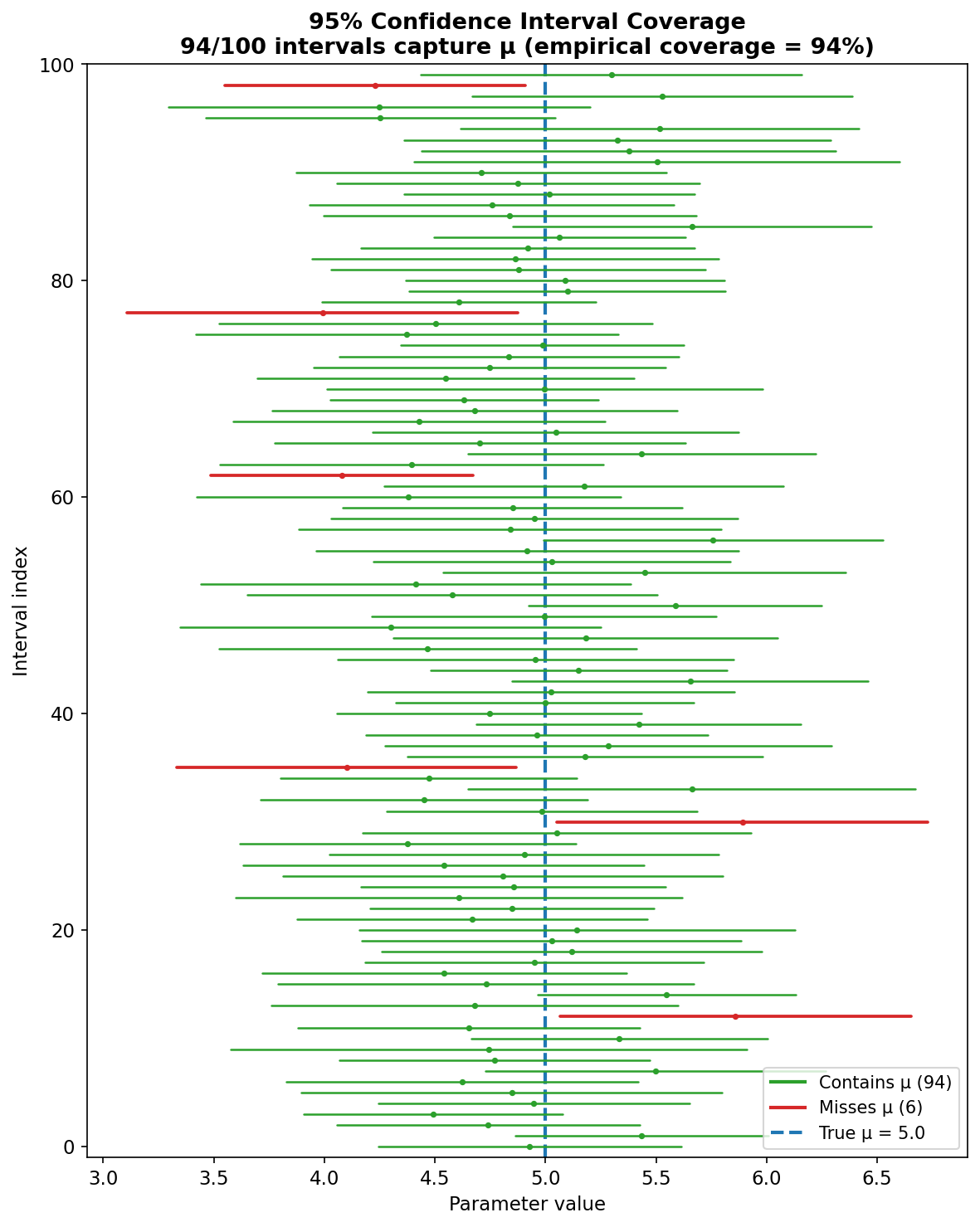
Fig. 280 Figure E.1: 100 independent 95% t-intervals for \(\mu = 5\) with \(n = 25\). Green intervals capture the true parameter (blue dashed line); red intervals miss. The empirical coverage (94/100) is consistent with the nominal 95% level.
When Coverage Breaks Down: The Wald Proportion Interval
The Wald interval for a binomial proportion, \(\hat{p} \pm z_{\alpha/2}\sqrt{\hat{p}(1-\hat{p})/n}\), is the textbook default but is notorious for poor coverage when \(n \cdot p\) is small. The Wilson interval corrects this by inverting the score test rather than the Wald test:
import numpy as np
from scipy import stats

rng = np.random.default_rng(42)

# Coverage investigation: Wald vs Wilson CI for small p
p_true = 0.05
n_reps = 50000
alpha = 0.05

print("Coverage of 95% CI for Binomial proportion (p = 0.05)")
print(f"{'n':>5}  {'n·p':>5}  {'Wald':>8}  {'Wilson':>8}")
print("-" * 35)

for n in [10, 20, 50, 200]:
    wald_cover = 0
    wilson_cover = 0
    for i in range(n_reps):
        x = rng.binomial(n, p_true)
        p_hat = x / n

        # Wald interval
        se_wald = np.sqrt(p_hat * (1 - p_hat) / n)
        lo_w = p_hat - 1.96 * se_wald
        hi_w = p_hat + 1.96 * se_wald
        if lo_w <= p_true <= hi_w:
            wald_cover += 1

        # Wilson interval
        z = 1.96
        denom = 1 + z**2 / n
        center = (p_hat + z**2 / (2*n)) / denom
        margin = z * np.sqrt(p_hat*(1-p_hat)/n + z**2/(4*n**2)) / denom
        lo_ws = center - margin
        hi_ws = center + margin
        if lo_ws <= p_true <= hi_ws:
            wilson_cover += 1

    print(f"{n:>5}  {n*p_true:>5.1f}  {wald_cover/n_reps:>8.3f}  "
          f"{wilson_cover/n_reps:>8.3f}")
Coverage of 95% CI for Binomial proportion (p = 0.05)
    n    n·p      Wald    Wilson
-----------------------------------
   10    0.5     0.403     0.914
   20    1.0     0.640     0.924
   50    2.5     0.922     0.963
  200   10.0     0.925     0.966
The Wald interval’s coverage is catastrophic when \(n \cdot p\) is small: only 40.3% coverage at \(n = 10\) (nominally 95%). The problem is fundamental — when \(\hat{p}\) can be exactly 0 (which happens with probability \(0.95^{10} \approx 0.60\) at \(n = 10\)), the Wald interval collapses to the point \([0, 0]\) and cannot capture the true \(p > 0\). The Wilson interval remains above 90% coverage even at \(n = 10\) because it uses the score test’s better small-sample behavior. Even at \(n = 200\), the Wald interval only reaches 92.5% — still below the nominal 95%.
Statistical Application
Chapter 4 introduces the bootstrap confidence interval, which does not require a pivotal quantity or distributional assumptions. The bootstrap resamples the data to approximate the sampling distribution directly. Understanding the frequentist coverage guarantee developed here is essential for evaluating bootstrap CI methods.
Hypothesis Testing
The Neyman-Pearson Framework
Hypothesis testing provides a formal decision procedure for choosing between competing claims about a parameter based on data.
Definition
A hypothesis test involves:
A null hypothesis \(H_0\) (the claim to be tested, often a “no effect” or “default” statement)
An alternative hypothesis \(H_1\) (the claim we adopt if the evidence against \(H_0\) is sufficiently strong)
A test statistic \(T(X_1, \ldots, X_n)\) that measures the discrepancy between the data and what \(H_0\) predicts
A rejection region \(R\): we reject \(H_0\) if \(T \in R\)
Hypotheses are simple if they specify \(\theta\) completely (e.g., \(H_0: \mu = 5\)) and composite if they specify a set of values (e.g., \(H_1: \mu > 5\)).
Intuition. Hypothesis testing is a decision procedure, not a belief-updating procedure. We fix a default claim (\(H_0\)) and ask: “Is the data so incompatible with \(H_0\) that a rational agent would abandon it?” The framework is asymmetric by design — we control the probability of wrongly rejecting \(H_0\) (Type I error) because false alarms typically have higher stakes than missed discoveries. The test statistic distills a high-dimensional dataset into a single number measuring departure from \(H_0\), and the rejection region determines how extreme that number must be before we act. This is analogous to a courtroom: \(H_0\) is “not guilty,” and we require evidence beyond a reasonable doubt (\(\alpha\)) before convicting.
Error Types and Power
Definition
Truth vs. Decision |
Do not reject \(H_0\) |
Reject \(H_0\) |
|---|---|---|
\(H_0\) true |
Correct decision |
Type I error (prob = α) |
\(H_0\) false |
Type II error (prob = β) |
Correct decision (power = 1−β) |
The significance level \(\alpha = P(\text{reject } H_0 \mid H_0 \text{ true})\) is the maximum Type I error rate. We control this by design.
The power of a test against a specific alternative \(\theta_1\) is \(\pi(\theta_1) = P(\text{reject } H_0 \mid \theta = \theta_1) = 1 - \beta(\theta_1)\). We want this to be large.
The power function \(\pi(\theta)\) gives the rejection probability as a function of the true parameter. At \(H_0\), \(\pi(\theta_0) = \alpha\); a good test has \(\pi(\theta)\) increasing rapidly as \(\theta\) moves away from \(H_0\).
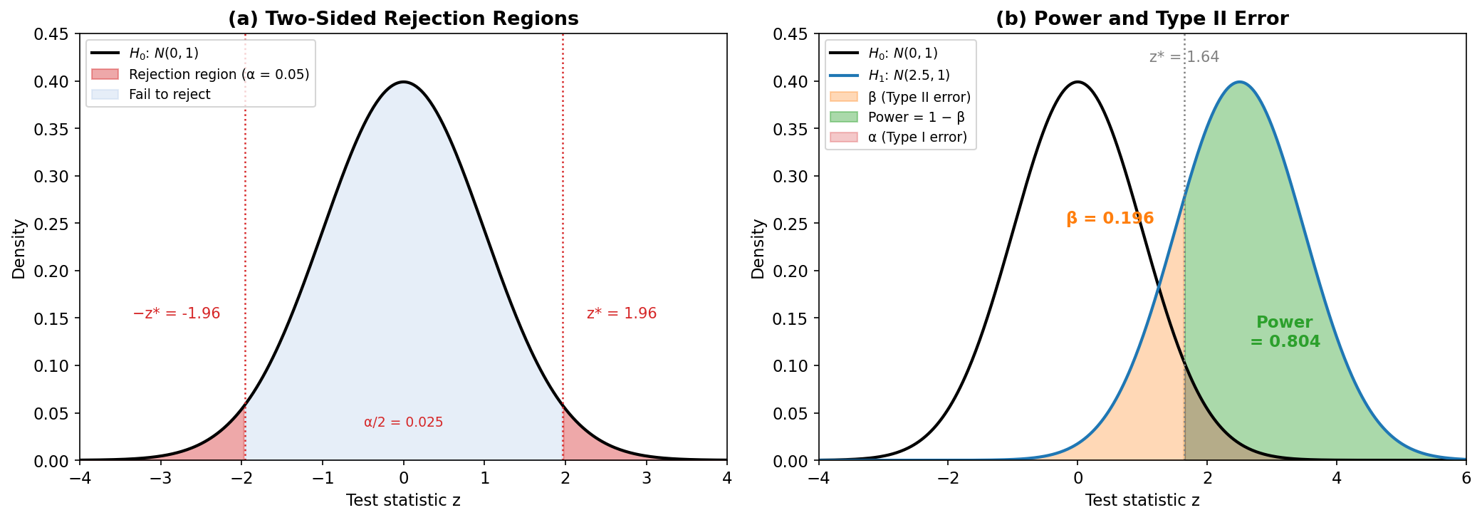
Fig. 281 Figure E.2: The geometry of hypothesis testing. (a) Two-sided rejection regions: the red shaded tails each contain \(\alpha/2 = 0.025\) of the null distribution, giving critical values \(\pm 1.96\). (b) Null (\(H_0\)) and alternative (\(H_1\)) distributions overlaid. The orange region is \(\beta\) (Type II error — failing to reject when \(H_1\) is true); the green region is power \(= 1 - \beta\). Moving the alternative further from the null shrinks \(\beta\) and increases power.
P-Values
Definition
The p-value is the probability, under \(H_0\), of observing a test statistic at least as extreme as the one actually observed:
For a two-sided test: \(p = P_{H_0}(|T| \ge |t_{\text{obs}}|)\).
Intuition. The p-value answers a specific question: “If \(H_0\) were true, how surprising is what we observed?” It measures surprise on the probability scale — a p-value of 0.03 means that under \(H_0\), only 3% of datasets would produce a test statistic as extreme or more extreme than ours. Critically, the p-value is not the probability that \(H_0\) is true (that is a Bayesian posterior probability requiring a prior), and it is not the probability that the result occurred “by chance” (the data already occurred). The p-value is a pre-experimental probability evaluated at the observed data: it calibrates how well \(H_0\) predicts what we saw. The decision rule “reject \(H_0\) when \(p < \alpha\)” is equivalent to “reject when \(T \in R\)” for any fixed \(\alpha\).
Theorem: P-Values are Uniform Under \(H_0\)
If the test statistic \(T\) has a continuous distribution under \(H_0\), then the p-value \(p = 1 - F_0(T)\) is uniformly distributed on \([0, 1]\) under \(H_0\).
Derivation
Let \(F_0\) be the CDF of \(T\) under \(H_0\). The one-sided p-value is \(p = 1 - F_0(T)\). We need \(P_{H_0}(p \le u) = u\) for \(u \in [0,1]\).
The key step is the probability integral transform: if \(T \sim F_0\), then \(F_0(T) \sim \text{Uniform}(0,1)\). This is why we can check for a uniform histogram of p-values under \(H_0\) to validate a test procedure.
Caution
What a p-value is NOT:
❌ The probability that \(H_0\) is true. P-values are computed assuming \(H_0\) is true — they cannot tell you the probability that this assumption is correct. This conflation is the “prosecutor’s fallacy”: \(P(\text{data} \mid H_0)\) is not \(P(H_0 \mid \text{data})\).
❌ The probability of “getting this result by chance.” The entire test is conducted under the assumption of chance (i.e., \(H_0\)); the p-value measures how extreme the observed result is under that assumption.
❌ The probability that rejecting \(H_0\) is a mistake. That would be \(P(H_0 \mid \text{reject})\), which depends on the prior probability of \(H_0\) — a Bayesian quantity.
import numpy as np
from scipy import stats

rng = np.random.default_rng(42)

# Simulate p-values under H₀ and H₁
mu0 = 0.0
sigma = 1.0
n = 25
n_reps = 10000

# Under H₀: μ = 0
pvals_h0 = np.zeros(n_reps)
for i in range(n_reps):
    sample = rng.normal(mu0, sigma, n)
    t_stat = np.mean(sample) / (np.std(sample, ddof=1) / np.sqrt(n))
    pvals_h0[i] = 2 * stats.t.sf(abs(t_stat), df=n-1)

# Under H₁: μ = 0.5
mu1 = 0.5
pvals_h1 = np.zeros(n_reps)
for i in range(n_reps):
    sample = rng.normal(mu1, sigma, n)
    t_stat = np.mean(sample) / (np.std(sample, ddof=1) / np.sqrt(n))
    pvals_h1[i] = 2 * stats.t.sf(abs(t_stat), df=n-1)

print("P-value distributions (two-sided t-test, n=25):")
print()
print("Under H₀ (μ = 0):")
print(f"  Mean p-value: {np.mean(pvals_h0):.4f} (theory: 0.5000)")
print(f"  Reject at α=0.05: {np.mean(pvals_h0 < 0.05):.4f} "
      f"(theory: 0.0500)")
print(f"  Reject at α=0.01: {np.mean(pvals_h0 < 0.01):.4f} "
      f"(theory: 0.0100)")
print(f"  Uniform check — fraction in [0.0, 0.1]: "
      f"{np.mean(pvals_h0 < 0.1):.4f} (theory: 0.1000)")
print(f"  Uniform check — fraction in [0.4, 0.6]: "
      f"{np.mean((pvals_h0 >= 0.4) & (pvals_h0 < 0.6)):.4f} "
      f"(theory: 0.2000)")
print()
print("Under H₁ (μ = 0.5, δ/σ = 0.5):")
print(f"  Mean p-value: {np.mean(pvals_h1):.4f}")
print(f"  Power at α=0.05: {np.mean(pvals_h1 < 0.05):.4f}")
print(f"  Power at α=0.01: {np.mean(pvals_h1 < 0.01):.4f}")
P-value distributions (two-sided t-test, n=25):

Under H₀ (μ = 0):
  Mean p-value: 0.5001 (theory: 0.5000)
  Reject at α=0.05: 0.0518 (theory: 0.0500)
  Reject at α=0.01: 0.0103 (theory: 0.0100)
  Uniform check — fraction in [0.0, 0.1]: 0.1021 (theory: 0.1000)
  Uniform check — fraction in [0.4, 0.6]: 0.1985 (theory: 0.2000)

Under H₁ (μ = 0.5, δ/σ = 0.5):
  Mean p-value: 0.0808
  Power at α=0.05: 0.6654
  Power at α=0.01: 0.3992
Under \(H_0\), the p-values behave exactly as the theorem predicts: uniform on [0, 1], with each decile containing approximately 10% of the mass. The rejection rate at \(\alpha = 0.05\) is 5.2%, confirming the Type I error rate. Under \(H_1\) with effect size \(\delta/\sigma = 0.5\) and \(n = 25\), the power at \(\alpha = 0.05\) is 66.5% — a medium-effect study with \(n = 25\) misses about one-third of true effects.
Power Analysis
Power depends on four quantities: the significance level \(\alpha\), the sample size \(n\), the effect size \(\delta = |\theta_1 - \theta_0|\), and the variability \(\sigma\). Specifying any three determines the fourth.
Derivation: Power of the One-Sample z-Test
Consider testing \(H_0: \mu = \mu_0\) versus \(H_1: \mu > \mu_0\) at level \(\alpha\), with \(\sigma\) known. The test rejects when \(Z = \frac{\bar{X} - \mu_0}{\sigma/\sqrt{n}} > z_\alpha\).
Under the alternative \(\mu = \mu_1 > \mu_0\):
The first term is \(\sim N(0,1)\) under \(\mu_1\), and the second is the non-centrality parameter \(\delta\sqrt{n}/\sigma\) where \(\delta = \mu_1 - \mu_0\). Thus under \(H_1\):
This is the power function. It increases with \(\delta\) (larger effects are easier to detect), with \(n\) (more data means more power), and decreases with \(\sigma\) (more noise means less power).
The following table shows simulated power (10,000 replicates) for the two-sided \(t\)-test at Cohen’s conventional effect size benchmarks:
\(\delta/\sigma\) |
\(n = 10\) |
\(n = 25\) |
\(n = 50\) |
\(n = 100\) |
|---|---|---|---|---|
0.0 |
0.051 |
0.050 |
0.051 |
0.048 |
0.2 (small) |
0.090 |
0.161 |
0.291 |
0.509 |
0.5 (medium) |
0.291 |
0.662 |
0.935 |
0.998 |
0.8 (large) |
0.617 |
0.970 |
1.000 |
1.000 |
1.0 |
0.807 |
0.998 |
1.000 |
1.000 |
At \(\delta/\sigma = 0\) (i.e., \(H_0\) is true), all sample sizes show rejection rates near 0.05, confirming the test’s level. A “small” effect (\(\delta/\sigma = 0.2\)) has only 29% power even at \(n = 50\) — such effects require \(n \ge 200\) for the conventional 80% power threshold. A “medium” effect (0.5) needs \(n \approx 35\) for 80% power, and a “large” effect (0.8) needs only \(n \approx 15\). These numbers have direct design implications: an underpowered study wastes resources by being unlikely to detect the effect it was designed to find.
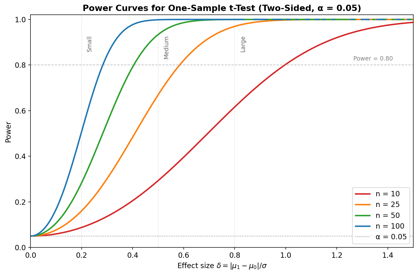
Fig. 282 Figure E.3: Power of the two-sided one-sample \(t\)-test as a function of effect size \(\delta/\sigma\) for \(n \in \{10, 25, 50, 100\}\) at \(\alpha = 0.05\). Cohen’s benchmarks (small = 0.2, medium = 0.5, large = 0.8) are marked. The dashed line at power = 0.80 is the conventional design threshold. Larger samples detect smaller effects: \(n = 100\) reaches 80% power at \(\delta/\sigma \approx 0.28\), while \(n = 10\) requires \(\delta/\sigma \approx 1.0\).
The Neyman-Pearson Lemma
The Neyman-Pearson lemma answers a fundamental question: among all level-\(\alpha\) tests of a simple null against a simple alternative, which is most powerful?
Intuition. If we must decide between two specific distributions \(f(\mathbf{x}; \theta_0)\) and \(f(\mathbf{x}; \theta_1)\), the most informative quantity is how much more likely the data are under one than the other — the likelihood ratio \(\Lambda(\mathbf{x}) = f(\mathbf{x};\theta_1)/f(\mathbf{x};\theta_0)\). Points with high \(\Lambda\) are strong evidence for \(\theta_1\); points with low \(\Lambda\) favor \(\theta_0\). The Neyman-Pearson lemma proves that no test can do better than simply thresholding \(\Lambda\): any other rejection region of the same size \(\alpha\) must capture less of the \(\theta_1\)-distribution. The proof is essentially an accounting argument — by moving probability mass from the NP rejection region to any other region, we always trade high-\(\Lambda\) points (which contribute more power per unit of \(\alpha\)) for low-\(\Lambda\) points (which contribute less). This optimality principle is why likelihood ratios appear at the foundation of virtually all testing theory.
Theorem: Neyman-Pearson Lemma
Let \(X_1, \ldots, X_n\) have joint density \(f(\mathbf{x}; \theta)\). For testing \(H_0: \theta = \theta_0\) versus \(H_1: \theta = \theta_1\), the most powerful level-\(\alpha\) test rejects \(H_0\) when the likelihood ratio exceeds a threshold:
where \(k\) is chosen so that \(P_{\theta_0}(\Lambda > k) = \alpha\).
Proof
Let \(\phi^*\) be the Neyman-Pearson test (reject when \(\Lambda > k\)) and \(\phi\) be any other level-\(\alpha\) test. We need to show \(\mathbb{E}_{\theta_1}[\phi^*] \ge \mathbb{E}_{\theta_1}[\phi]\).
Consider:
In the rejection region of \(\phi^*\), we have \(f(\mathbf{x}; \theta_1) > k \cdot f(\mathbf{x}; \theta_0)\) and \(\phi^* = 1\), so \(\phi^* - \phi \ge 0\). In the acceptance region, \(f(\mathbf{x}; \theta_1) \le k \cdot f(\mathbf{x}; \theta_0)\) and \(\phi^* = 0\), so \(\phi^* - \phi \le 0\). Therefore:
Integrating:
Expanding:
since \(\mathbb{E}_{\theta_0}[\phi] \le \alpha\) (both tests are level-\(\alpha\)). Therefore \(\mathbb{E}_{\theta_1}[\phi^*] \ge \mathbb{E}_{\theta_1}[\phi]\), and \(\phi^*\) is the most powerful test.
The lemma tells us that likelihood ratios are the natural currency of hypothesis testing. For simple vs simple hypotheses, the LR test is provably optimal.
Uniformly Most Powerful Tests
For composite alternatives (\(H_1: \theta > \theta_0\)), a test is uniformly most powerful (UMP) at level \(\alpha\) if it is the most powerful test against every \(\theta_1 > \theta_0\) simultaneously.
Definition
A family of densities \(f(x;\theta)\) has monotone likelihood ratio (MLR) in a statistic \(T(x)\) if for \(\theta_1 > \theta_0\), the ratio \(f(\mathbf{x};\theta_1)/f(\mathbf{x};\theta_0)\) is a non-decreasing function of \(T(\mathbf{x})\). All one-parameter exponential families have MLR in the natural sufficient statistic.
Theorem: Karlin-Rubin
If the family has MLR in \(T\), then the test that rejects \(H_0: \theta \le \theta_0\) when \(T > c\) (where \(c\) satisfies \(P_{\theta_0}(T > c) = \alpha\)) is UMP at level \(\alpha\) for \(H_1: \theta > \theta_0\).
Proof Sketch
By the Neyman-Pearson lemma, the most powerful test of \(H_0: \theta = \theta_0\) versus any simple \(H_1: \theta = \theta_1 > \theta_0\) rejects when \(\Lambda = f(\mathbf{x};\theta_1)/f(\mathbf{x};\theta_0) > k\). Since the family has MLR in \(T\), \(\Lambda > k\) is equivalent to \(T > c\) for some \(c\). Crucially, the threshold \(c\) is determined by the size constraint \(P_{\theta_0}(T > c) = \alpha\), which does not depend on \(\theta_1\). Therefore the same rejection region \(\{T > c\}\) is most powerful against every \(\theta_1 > \theta_0\) — it is UMP.
Example: For Poisson(\(\lambda\)) data, testing \(H_0: \lambda \le \lambda_0\) versus \(H_1: \lambda > \lambda_0\), the UMP test rejects when \(\sum X_i > c\). No test can do better for one-sided alternatives.
Non-existence of two-sided UMP tests. For two-sided alternatives (\(H_1: \theta \ne \theta_0\)), a UMP test generally does not exist. A test that is powerful against \(\theta_1 > \theta_0\) (rejecting for large \(T\)) sacrifices power against \(\theta_1 < \theta_0\). The two-sided \(t\)-test is a practical compromise, splitting \(\alpha\) between both tails, but it is not UMP. The likelihood ratio test provides a principled approach to two-sided and multiparameter problems.
Common Hypothesis Tests
One-sample t-test. For \(H_0: \mu = \mu_0\) with unknown \(\sigma\):
Reject \(H_0\) if \(|T| > t_{\alpha/2,\, n-1}\) (two-sided) or \(T > t_{\alpha,\, n-1}\) (one-sided).
Two-sample t-test. For \(H_0: \mu_1 = \mu_2\) with independent samples of sizes \(n_1, n_2\):
where \(S_p^2\) is the pooled variance. Under \(H_0\) with equal variances: \(T \sim t_{n_1+n_2-2}\).
Paired t-test. For matched pairs \((X_i, Y_i)\), define \(D_i = X_i - Y_i\) and test \(H_0: \mu_D = 0\):
Chi-squared goodness-of-fit test. For testing whether observed counts \(O_1, \ldots, O_k\) match expected counts \(E_1, \ldots, E_k\):
where \(p\) is the number of parameters estimated from the data. The approximation requires \(E_j \ge 5\) for all cells (a rough guideline).
F-test for equal variances. For \(H_0: \sigma_1^2 = \sigma_2^2\) with independent normal samples:
The F-distribution also arises in ANOVA and regression (testing whether groups of coefficients are jointly zero).
Multiple Testing
When conducting \(m\) hypothesis tests simultaneously, the probability of at least one false rejection grows rapidly even if each individual test controls \(\alpha\).
Definition
Family-wise error rate (FWER): \(P(\text{at least one false rejection})\). With \(m\) independent tests at level \(\alpha\): \(\text{FWER} = 1 - (1-\alpha)^m\). For \(m = 20\) at \(\alpha = 0.05\): \(\text{FWER} = 0.64\).
False discovery rate (FDR): \(\mathbb{E}\!\left[\frac{\text{false rejections}}{\text{total rejections}}\right]\), with \(0/0 = 0\) by convention. The FDR controls the expected proportion of false discoveries, making it less conservative than FWER control.
Bonferroni correction. Reject the \(i\)-th null when \(p_i < \alpha/m\). This controls \(\text{FWER} \le \alpha\) (by the union bound) but is conservative — it substantially reduces power.
Benjamini-Hochberg (BH) procedure. Sort p-values: \(p_{(1)} \le \cdots \le p_{(m)}\). Find the largest \(k\) such that \(p_{(k)} \le \frac{k}{m}\alpha\). Reject all \(H_{(1)}, \ldots, H_{(k)}\). This controls \(\text{FDR} \le \alpha\) (under independence or positive regression dependency) while retaining more power than Bonferroni.
import numpy as np
from scipy import stats

rng = np.random.default_rng(42)

# Multiple testing demo
n_tests = 200
n_true_null = 180
n_true_alt = 20
delta = 0.5
n_per_test = 30
alpha = 0.05

p_values = np.zeros(n_tests)
is_null = np.zeros(n_tests, dtype=bool)
is_null[:n_true_null] = True

for i in range(n_tests):
    if is_null[i]:
        sample = rng.normal(0, 1, n_per_test)
    else:
        sample = rng.normal(delta, 1, n_per_test)
    t_stat = (np.mean(sample)
              / (np.std(sample, ddof=1) / np.sqrt(n_per_test)))
    p_values[i] = 2 * stats.t.sf(abs(t_stat), df=n_per_test-1)

# Bonferroni
bonf_reject = p_values < alpha / n_tests

# Benjamini-Hochberg
sorted_idx = np.argsort(p_values)
sorted_p = p_values[sorted_idx]
m = n_tests
bh_threshold = np.arange(1, m+1) * alpha / m
bh_reject_sorted = np.zeros(m, dtype=bool)
k_max = 0
for k in range(m):
    if sorted_p[k] <= bh_threshold[k]:
        k_max = k + 1
bh_reject_sorted[:k_max] = True
bh_reject = np.zeros(m, dtype=bool)
bh_reject[sorted_idx] = bh_reject_sorted

# Unadjusted
raw_reject = p_values < alpha

def metrics(reject, is_null):
    fp = np.sum(reject & is_null)
    tp = np.sum(reject & ~is_null)
    total = np.sum(reject)
    fdr = fp / total if total > 0 else 0
    power = tp / np.sum(~is_null)
    fwer = 1 if fp > 0 else 0
    return total, fp, tp, fdr, power, fwer

print(f"Multiple testing: {n_tests} tests "
      f"({n_true_null} true nulls, "
      f"{n_true_alt} alternatives with δ={delta})")
print(f"Each test: two-sided t-test with n={n_per_test}")
print()
print(f"{'Method':>15}  {'Rejected':>8}  {'FP':>4}  "
      f"{'TP':>4}  {'FDR':>7}  {'Power':>7}  {'FWER':>5}")
print("-" * 60)

for name, reject in [("Unadjusted", raw_reject),
                      ("Bonferroni", bonf_reject),
                      ("BH (FDR)", bh_reject)]:
    total, fp, tp, fdr, power, fwer = metrics(reject, is_null)
    print(f"{name:>15}  {total:>8}  {fp:>4}  {tp:>4}  "
          f"{fdr:>7.3f}  {power:>7.3f}  {fwer:>5}")
Multiple testing: 200 tests (180 true nulls, 20 alternatives with δ=0.5)
Each test: two-sided t-test with n=30

         Method  Rejected    FP    TP      FDR    Power   FWER
------------------------------------------------------------
     Unadjusted        25    11    14    0.440    0.700      1
     Bonferroni         5     0     5    0.000    0.250      0
       BH (FDR)         8     0     8    0.000    0.400      0
The tradeoff is stark. Unadjusted testing rejects 25 hypotheses with 70% power, but 44% of its discoveries are false (11 out of 25). Bonferroni eliminates all false positives but only finds 5 of the 20 true effects (25% power). BH strikes a middle ground: zero false discoveries in this realization while recovering 8 of the 20 effects. In repeated realizations, BH would allow some false discoveries but controls their expected proportion at \(\le \alpha = 0.05\).
Statistical Application
The Neyman-Pearson lemma motivates the likelihood ratio test developed in Section 3.2 Maximum Likelihood Estimation. The Wald and score tests are asymptotic approximations to the LRT, all sharing the same \(\chi^2\) limiting distribution. Multiple testing corrections are critical in genomics, A/B testing, and any setting where many hypotheses are tested simultaneously.
Sufficiency and Information
Sufficient Statistics
Definition
A statistic \(T(\mathbf{X})\) is sufficient for \(\theta\) if the conditional distribution of the data \(\mathbf{X}\) given \(T(\mathbf{X}) = t\) does not depend on \(\theta\).
Intuitively, a sufficient statistic captures everything the data can tell us about \(\theta\). Once we know \(T\), the remaining randomness in \(\mathbf{X}\) is pure noise — no further information about \(\theta\) is available. This is a powerful idea: we can reduce an entire dataset to a (usually low-dimensional) summary without losing any information about the parameter.
The Fisher-Neyman Factorization Theorem
Checking the definition of sufficiency directly (computing conditional distributions) is usually difficult. The factorization theorem provides an elegant shortcut.
Theorem: Fisher-Neyman Factorization
A statistic \(T(\mathbf{X})\) is sufficient for \(\theta\) if and only if the joint density (or PMF) can be written as
where \(g\) depends on \(\mathbf{x}\) only through \(T(\mathbf{x})\), and \(h\) does not depend on \(\theta\).
Proof (Discrete Case)
Sufficiency ⟹ Factorization. If \(T\) is sufficient, then \(P(\mathbf{X} = \mathbf{x} \mid T = t)\) does not depend on \(\theta\). Write:
where \(t = T(\mathbf{x})\). Set \(g(t, \theta) = P(T = t; \theta)\) and \(h(\mathbf{x}) = P(\mathbf{X} = \mathbf{x} \mid T = T(\mathbf{x}))\).
Factorization ⟹ Sufficiency. If \(f(\mathbf{x}; \theta) = g(T(\mathbf{x}), \theta) \cdot h(\mathbf{x})\), then:
The \(g(t,\theta)\) cancels, so the conditional distribution does not depend on \(\theta\).
Examples of Sufficient Statistics
Normal \((\mu, \sigma^2)\): The joint density is
The exponent depends on \(\mathbf{x}\) only through \((\sum x_i, \sum x_i^2)\), so \(T = (\bar{X}, S^2)\) — equivalently \((\sum X_i, \sum X_i^2)\) — is jointly sufficient for \((\mu, \sigma^2)\).
Poisson \((\lambda)\): \(f(\mathbf{x}; \lambda) = \prod \frac{\lambda^{x_i} e^{-\lambda}}{x_i!} = \frac{\lambda^{\sum x_i} e^{-n\lambda}}{\prod x_i!}\). The \(\theta\)-dependent part involves \(\mathbf{x}\) only through \(\sum x_i\), so \(T = \sum X_i\) is sufficient for \(\lambda\).
Uniform \((0, \theta)\): \(f(\mathbf{x}; \theta) = \theta^{-n} \cdot \prod \mathbf{1}(0 \le x_i \le \theta) = \theta^{-n} \cdot \mathbf{1}(x_{(n)} \le \theta) \cdot \prod \mathbf{1}(x_i \ge 0)\). The \(\theta\)-dependent part involves \(\mathbf{x}\) only through \(x_{(n)} = \max(x_i)\), so \(T = X_{(n)}\) is sufficient for \(\theta\).
Minimal Sufficiency
A sufficient statistic is minimal sufficient if it achieves the greatest data reduction — it is a function of every other sufficient statistic. To find a minimal sufficient statistic, use the likelihood ratio method: \(T(\mathbf{x}) = T(\mathbf{y})\) if and only if the ratio \(f(\mathbf{x};\theta)/f(\mathbf{y};\theta)\) does not depend on \(\theta\).
For example, for Normal \((\mu, \sigma^2)\), computing \(f(\mathbf{x};\mu,\sigma^2)/f(\mathbf{y};\mu,\sigma^2)\) shows the ratio is free of \((\mu, \sigma^2)\) exactly when \(\bar{x} = \bar{y}\) and \(\sum x_i^2 = \sum y_i^2\), confirming that \((\bar{X}, \sum X_i^2)\) is minimal sufficient.
Completeness
Definition
A family of distributions for a statistic \(T\) is complete if \(\mathbb{E}_\theta[g(T)] = 0\) for all \(\theta\) implies \(P_\theta(g(T) = 0) = 1\) for all \(\theta\).
Completeness means the sufficient statistic carries no “wasted” randomness — there is no non-trivial function of \(T\) that is identically zero in expectation across all parameter values. For exponential families with open natural parameter spaces, the natural sufficient statistic is always complete. This includes Normal, Poisson, Binomial, Exponential, Gamma, and Beta families.
Completeness is the key ingredient that, combined with sufficiency, yields the UMVUE through the Lehmann-Scheffé theorem (stated in the Point Estimation section above): if \(T\) is complete sufficient and \(h(T)\) is unbiased for \(g(\theta)\), then \(h(T)\) is the unique UMVUE.
Ancillary Statistics and Basu’s Theorem
Definition
A statistic \(A(\mathbf{X})\) is ancillary for \(\theta\) if its distribution does not depend on \(\theta\). Ancillary statistics carry no information about \(\theta\) on their own, yet they can affect the precision of other estimators.
Example: For \(X_1, \ldots, X_n \sim N(\mu, 1)\), the sample range \(R = X_{(n)} - X_{(1)}\) is ancillary for \(\mu\): shifting all observations by a constant changes \(\bar{X}\) but not \(R\). While \(R\) tells us nothing about \(\mu\) directly, it indicates how spread out the sample is, which affects how precisely \(\bar{X}\) estimates \(\mu\).
Theorem: Basu’s Theorem
If \(T\) is a complete sufficient statistic and \(A\) is ancillary, then \(T\) and \(A\) are independent. (Proof omitted.)
Basu’s theorem is elegant: it says that a complete sufficient statistic and an ancillary statistic live in “orthogonal” parts of the sample space. This has practical consequences — for example, for \(X_1, \ldots, X_n \sim N(\mu, \sigma^2)\) with \(\sigma^2\) known, \(\bar{X}\) is complete sufficient for \(\mu\) while \(S^2\) is ancillary (its distribution \(\sigma^2 \chi^2_{n-1}/(n-1)\) does not involve \(\mu\)), so Basu’s theorem delivers the independence of \(\bar{X}\) and \(S^2\) — the key fact behind the \(t\)-distribution — without any calculation.
Fisher Information
Fisher information quantifies how much information a single observation carries about \(\theta\).
Intuition. Consider the log-likelihood \(\ell(\theta)\) as a landscape over the parameter space. At the true \(\theta\), the log-likelihood is (on average) at its peak. Fisher information measures the curvature of this peak: a sharp, narrow peak means the data are highly informative (the likelihood strongly distinguishes nearby parameter values), while a broad, flat peak means the data carry little information (many parameter values are nearly equally plausible). Formally, Fisher information is the expected curvature \(-\mathbb{E}[\ell''(\theta)]\), or equivalently, the variance of the score. High curvature means the score changes rapidly — the derivative of the log-likelihood is volatile across samples — which means the data are highly sensitive to \(\theta\). This geometric picture directly connects to estimation precision: sharper peaks yield more precise estimators, a relationship made exact by the Cramér-Rao bound below.
Definition
The score function is the gradient of the log-likelihood with respect to \(\theta\):
The Fisher information for a single observation is:
The second equality holds because \(\mathbb{E}[U(\theta)] = 0\) (proved below).
Notation Convention
\(I_1(\theta)\) = Fisher information from a single observation
\(I_n(\theta) = n \cdot I_1(\theta)\) = total Fisher information from \(n\) iid observations
\(I(\theta) = -\mathbb{E}\!\left[\frac{\partial^2 \ell}{\partial \theta^2}\right]\) = expected (Fisher) information
\(J(\hat{\theta}) = -\frac{\partial^2 \ell}{\partial \theta^2}\big|_{\hat{\theta}}\) = observed information (data-dependent, evaluated at the MLE)
Under correct model specification, \(\mathbb{E}[J(\theta_0)] = I(\theta_0)\). Under misspecification, these may differ — see Section 3.2 Maximum Likelihood Estimation for the sandwich variance estimator.
Theorem: \(\mathbb{E}[U(\theta)] = 0\)
Under regularity conditions (interchange of differentiation and integration), the expected score is zero.
Proof
Since \(\int f(x; \theta)\, dx = 1\) for all \(\theta\), differentiating both sides with respect to \(\theta\):
Two Equivalent Forms of Fisher Information
Theorem
Under regularity conditions:
That is, Fisher information equals the variance of the score, and also equals the negative expected curvature of the log-likelihood.
Proof of Equivalence
Starting from \(\mathbb{E}[U(\theta)] = 0 = \int \frac{\partial}{\partial\theta}\log f(x;\theta) \cdot f(x;\theta)\, dx\), differentiate again with respect to \(\theta\):
since \(\frac{\partial f}{\partial\theta} = f \cdot \frac{\partial \log f}{\partial\theta}\). Therefore:
The left side is \(\text{Var}(U(\theta))\) (since \(\mathbb{E}[U] = 0\)), and the right side is \(-\mathbb{E}[\ell''(\theta)]\). Both equal \(I_1(\theta)\).
The second form is often easier to compute: take the second derivative of the log-likelihood and negate its expectation. The first form (score variance) is more natural for simulation-based verification.
Additive property. For an iid sample of size \(n\): \(I_n(\theta) = n \cdot I_1(\theta)\). The total information scales linearly with \(n\) — this is why standard errors shrink like \(1/\sqrt{n}\).
Fisher information for common distributions:
Distribution |
Parameter |
\(I_1(\theta)\) |
|---|---|---|
Bernoulli(\(p\)) |
\(p\) |
\(\frac{1}{p(1-p)}\) |
Poisson(\(\lambda\)) |
\(\lambda\) |
\(\frac{1}{\lambda}\) |
Normal(\(\mu, \sigma^2\) known) |
\(\mu\) |
\(\frac{1}{\sigma^2}\) |
Exponential(\(\lambda\)) |
\(\lambda\) |
\(\frac{1}{\lambda^2}\) |
import numpy as np
from scipy import stats

rng = np.random.default_rng(42)

# Verify Fisher information via simulated score variance
n_samples = 50000

print("Fisher information verification via score variance")
print(f"({n_samples:,} single-observation samples)")
print()
print(f"{'Distribution':>20}  {'I₁(θ) theory':>13}  "
      f"{'Var(score) sim':>15}  {'Ratio':>7}")
print("-" * 70)

# Poisson(λ=3): score = x/λ - 1, I₁ = 1/λ
lam = 3.0
x = rng.poisson(lam, n_samples)
score = x / lam - 1
theory = 1.0 / lam
sim = np.var(score)
print(f"{'Poisson(λ=3)':>20}  {theory:>13.6f}  "
      f"{sim:>15.6f}  {sim/theory:>7.4f}")

# Normal(μ=5, σ²=4): score = (x-μ)/σ², I₁ = 1/σ²
mu, sigma2 = 5.0, 4.0
x = rng.normal(mu, np.sqrt(sigma2), n_samples)
score = (x - mu) / sigma2
theory = 1.0 / sigma2
sim = np.var(score)
print(f"{'Normal(μ=5, σ²=4)':>20}  {theory:>13.6f}  "
      f"{sim:>15.6f}  {sim/theory:>7.4f}")

# Exp(λ=2): score = 1/λ - x, I₁ = 1/λ²
lam_exp = 2.0
x = rng.exponential(1.0/lam_exp, n_samples)
score = 1.0/lam_exp - x
theory = 1.0 / lam_exp**2
sim = np.var(score)
print(f"{'Exp(λ=2)':>20}  {theory:>13.6f}  "
      f"{sim:>15.6f}  {sim/theory:>7.4f}")

# Bernoulli(p=0.3): score = x/p - (1-x)/(1-p), I₁ = 1/(p(1-p))
p = 0.3
x = rng.binomial(1, p, n_samples)
score = x/p - (1-x)/(1-p)
theory = 1.0 / (p * (1-p))
sim = np.var(score)
print(f"{'Bernoulli(p=0.3)':>20}  {theory:>13.6f}  "
      f"{sim:>15.6f}  {sim/theory:>7.4f}")
Fisher information verification via score variance
(50,000 single-observation samples)

        Distribution   I₁(θ) theory   Var(score) sim    Ratio
----------------------------------------------------------------------
        Poisson(λ=3)       0.333333         0.334244   1.0027
   Normal(μ=5, σ²=4)       0.250000         0.247060   0.9882
            Exp(λ=2)       0.250000         0.249684   0.9987
    Bernoulli(p=0.3)       4.761905         4.756090   0.9988
All ratios are within 1.2% of 1.0, confirming the theoretical Fisher information values. The small deviations are simulation noise from 50,000 samples.
The Cramér-Rao Lower Bound
Theorem: Cramér-Rao Lower Bound (CRLB)
Let \(T = T(X_1, \ldots, X_n)\) be any unbiased estimator of \(\tau(\theta)\), a differentiable function of the parameter, based on an iid sample of size \(n\). Under regularity conditions — R4–R6 (differentiability, interchange of differentiation and integration, finite Fisher information) of the regularity conditions stated in the Asymptotic Theory section:
For estimating \(\theta\) itself (\(\tau(\theta) = \theta\), so \(\tau'(\theta) = 1\)):
No unbiased estimator can have variance below this bound. An estimator achieving equality is called efficient.
Intuition. The CRLB says there is a fundamental speed limit on estimation precision: no matter how clever our unbiased estimator, the data themselves impose a floor on how precise we can be. The bound is \(1/(nI_1(\theta))\) — inversely proportional to both the sample size and the per-observation information. This makes sense: more data and more informative observations both shrink the bound. The proof uses the Cauchy-Schwarz inequality to show that the correlation between any unbiased estimator and the score function is constrained, and this constraint propagates directly into a variance lower bound. When an estimator achieves equality (is efficient), it extracts every last bit of information from the data — it is perfectly correlated with the score. For exponential families, the natural sufficient statistic achieves this; for other families, no unbiased estimator may reach the bound, but the MLE approaches it as \(n \to \infty\).
Proof via Cauchy-Schwarz
Let \(U_n(\theta) = \sum_{i=1}^n \frac{\partial}{\partial\theta}\log f(X_i;\theta)\) be the total score. We know \(\mathbb{E}[U_n] = 0\) and \(\text{Var}(U_n) = n\,I_1(\theta)\). Let \(T\) be an unbiased estimator of \(\tau(\theta)\).
Step 1: Differentiate the unbiasedness condition. Since \(\mathbb{E}_\theta[T] = \tau(\theta)\):
Differentiating both sides with respect to \(\theta\) and using \(\frac{\partial f}{\partial\theta} = f \cdot \frac{\partial \log f}{\partial\theta}\):
Step 2: Compute the covariance. Since \(\mathbb{E}[U_n] = 0\):
Step 3: Apply Cauchy-Schwarz. For any random variables \(A, B\): \([\text{Cov}(A,B)]^2 \le \text{Var}(A) \cdot \text{Var}(B)\). Applied to \(T\) and \(U_n\):
Rearranging: \(\text{Var}(T) \ge \frac{[\tau'(\theta)]^2}{n\,I_1(\theta)}\). For \(\tau(\theta) = \theta\), this gives \(\text{Var}(\hat{\theta}) \ge \frac{1}{n\,I_1(\theta)}\). Equality holds iff \(T\) is an affine function of \(U_n\), which occurs precisely for exponential family distributions with their natural sufficient statistics.
When is the CRLB achieved? For exponential family distributions, the MLE achieves the CRLB exactly. For example, \(\bar{X}\) for Normal \((\mu)\) has \(\text{Var}(\bar{X}) = \sigma^2/n = 1/(n \cdot 1/\sigma^2) = 1/(n\,I_1(\mu))\). For non-exponential families, no unbiased estimator may achieve the bound, but the MLE approaches it asymptotically (see the Asymptotic Theory section below).
import numpy as np

rng = np.random.default_rng(42)

# Verify CRLB: Var(x̄) vs 1/(n·I₁) for Poisson(λ=3)
lam = 3.0
I1 = 1.0 / lam
n_reps = 50000

print("CRLB verification: Var(x̄) vs 1/(nI₁) for Poisson(λ=3)")
print(f"I₁(λ) = 1/λ = {I1:.6f}")
print()
print(f"{'n':>6}  {'Var(x̄) sim':>12}  "
      f"{'CRLB = 1/(nI₁)':>16}  {'Ratio':>7}")
print("-" * 50)

for n in [10, 25, 50, 100, 500]:
    xbar = np.zeros(n_reps)
    for i in range(n_reps):
        xbar[i] = np.mean(rng.poisson(lam, n))
    var_sim = np.var(xbar)
    crlb = 1.0 / (n * I1)
    print(f"{n:>6}  {var_sim:>12.6f}  {crlb:>16.6f}  "
          f"{var_sim/crlb:>7.4f}")
CRLB verification: Var(x̄) vs 1/(nI₁) for Poisson(λ=3)
I₁(λ) = 1/λ = 0.333333

     n   Var(x̄) sim    CRLB = 1/(nI₁)    Ratio
--------------------------------------------------
    10      0.296462          0.300000   0.9882
    25      0.118517          0.120000   0.9876
    50      0.059987          0.060000   0.9998
   100      0.029772          0.030000   0.9924
   500      0.006016          0.006000   1.0026
The variance of \(\bar{X}\) matches the CRLB to within 1.2% at every sample size — this is no coincidence. The Poisson is an exponential family, and \(\bar{X}\) is the MLE for \(\lambda\), so it achieves the CRLB exactly. The tiny deviations are purely simulation error.
Efficiency of Estimators
Not all estimators are equally efficient. The following comparison illustrates efficiency loss when using a suboptimal estimator.
import numpy as np

rng = np.random.default_rng(42)

# Efficiency comparison: Exp(λ) — MLE vs median-based
lam_true = 2.0
n = 50
n_reps = 50000

mle_est = np.zeros(n_reps)
med_est = np.zeros(n_reps)

for i in range(n_reps):
    sample = rng.exponential(1.0/lam_true, n)
    mle_est[i] = 1.0 / np.mean(sample)
    med_est[i] = np.log(2) / np.median(sample)

I1 = 1.0 / lam_true**2
crlb = 1.0 / (n * I1)

print(f"Efficiency comparison: Exp(λ={lam_true}), n={n}")
print(f"CRLB = 1/(nI₁) = {crlb:.6f}")
print()
print(f"{'Estimator':>20}  {'Mean':>8}  {'Var':>10}  "
      f"{'MSE':>10}  {'Rel. Eff.':>10}")
print("-" * 65)

mle_var = np.var(mle_est)
mle_mse = np.mean((mle_est - lam_true)**2)
med_var = np.var(med_est)
med_mse = np.mean((med_est - lam_true)**2)

print(f"{'MLE (1/x̄)':>20}  {np.mean(mle_est):>8.4f}  "
      f"{mle_var:>10.6f}  {mle_mse:>10.6f}  {1.0:>10.4f}")
print(f"{'Median (log2/med)':>20}  {np.mean(med_est):>8.4f}  "
      f"{med_var:>10.6f}  {med_mse:>10.6f}  "
      f"{mle_var/med_var:>10.4f}")
print()
print(f"Theoretical asymptotic relative efficiency: "
      f"{np.log(2)**2:.4f}")
Efficiency comparison: Exp(λ=2.0), n=50
CRLB = 1/(nI₁) = 0.080000

           Estimator      Mean         Var         MSE   Rel. Eff.
-----------------------------------------------------------------
          MLE (1/x̄)    2.0417    0.086203    0.087938      1.0000
   Median (log2/med)    2.0550    0.182654    0.185678      0.4719

Theoretical asymptotic relative efficiency: 0.4805
The median-based estimator has more than twice the variance of the MLE. The simulated relative efficiency (0.47) matches the theoretical asymptotic value \((\ln 2)^2 \approx 0.48\). Intuitively, the median discards information from the tails of the distribution, whereas the MLE uses all observations through the sample mean. To achieve the same precision as the MLE with \(n = 50\), the median-based estimator would need \(n \approx 50/0.48 \approx 104\) observations.
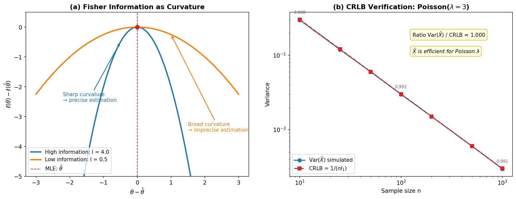
Fig. 283 Figure E.4: Fisher Information and the Cramér-Rao Bound. (a) High-information vs low-information settings: a sharp log-likelihood peak (small variance, high curvature) corresponds to high Fisher information, while a broad peak (large variance, low curvature) corresponds to low Fisher information. (b) CRLB verification: simulated variance of \(\bar{X}\) for Poisson(\(\lambda = 3\)) matches the theoretical bound \(1/(nI_1)\) across sample sizes, confirming that the MLE achieves the CRLB for exponential families.
Statistical Application
Sufficiency and Fisher information are the theoretical backbone of Section 3.2 Maximum Likelihood Estimation. The score equation \(U(\hat{\theta}) = 0\) defines the MLE, the observed information \(-\ell''(\hat{\theta})\) provides standard errors, and the CRLB establishes the best-case precision. The asymptotic efficiency of MLEs (proved in the Asymptotic Theory section below) means they approach the CRLB as \(n \to \infty\).
The Likelihood Function
Likelihood versus Probability
Definition
Given observed data \(\mathbf{x} = (x_1, \ldots, x_n)\), the likelihood function is
and the log-likelihood is
The likelihood and the density are the same mathematical expression, but they play fundamentally different roles:
Density \(f(x; \theta)\): \(\theta\) is fixed, \(x\) varies. Answers “how probable is \(x\)?”
Likelihood \(L(\theta; \mathbf{x})\): \(\mathbf{x}\) is fixed (observed), \(\theta\) varies. Answers “how well does \(\theta\) explain the data?”
The likelihood is not a probability distribution over \(\theta\) — it need not integrate to 1, and in general it does not. Only ratios of likelihoods are meaningful: \(L(\theta_1)/L(\theta_2)\) compares how well two parameter values explain the same data.
Why log-likelihood? Working with \(\ell(\theta) = \log L(\theta)\) has three advantages:
Numerical stability: Products of many small probabilities underflow; sums of log-probabilities do not.
Analytical convenience: Sums are easier to differentiate than products.
Concavity: For exponential families, \(\ell(\theta)\) is concave, guaranteeing a unique maximum.
Since \(\log\) is monotone increasing, maximizing \(L(\theta)\) and \(\ell(\theta)\) give the same answer.
Maximum Likelihood Estimation
Definition
The maximum likelihood estimator (MLE) \(\hat{\theta}_{\text{MLE}}\) is the parameter value that maximizes the likelihood:
Under regularity conditions, the MLE is found by solving the score equation \(U(\hat{\theta}) = 0\), where \(U(\theta) = \ell'(\theta) = \frac{\partial \ell}{\partial\theta}\).
Intuition. The MLE answers the question: “Which parameter value makes the observed data most probable?” This is a fundamentally different question from “What is the most probable parameter value?” (the latter requires a Bayesian prior). The MLE principle is agnostic about prior beliefs — it simply finds the parameter that best explains what happened. The score equation \(U(\hat{\theta}) = 0\) says the log-likelihood is flat at the MLE: moving \(\theta\) slightly in either direction does not improve the fit. The MLE has a remarkable collection of asymptotic properties — consistency, normality, and efficiency — that make it the workhorse of parametric inference (see the Asymptotic Theory section below). Its main limitation is that it requires a correctly specified parametric model; under misspecification, it converges to the parameter value closest to the truth in a Kullback-Leibler sense (Exercise 3d).
MLE for Poisson. Let \(X_1, \ldots, X_n \sim \text{Poisson}(\lambda)\). The log-likelihood is:
Differentiating and setting to zero:
Confirming this is a maximum: \(\ell''(\lambda) = -\sum x_i / \lambda^2 < 0\).
MLE for Normal. Let \(X_1, \ldots, X_n \sim N(\mu, \sigma^2)\). The log-likelihood is:
Taking partial derivatives and setting to zero:
Note that the MLE for \(\sigma^2\) uses \(1/n\) (not \(1/(n-1)\)), so it is the biased variance estimator. The MLE maximizes the likelihood but does not guarantee unbiasedness — the bias \(-\sigma^2/n\) vanishes as \(n \to \infty\).
MLE for Gamma. For Gamma(\(\alpha, \beta\)), the score equations have no closed-form solution — \(\hat{\alpha}\) satisfies a transcendental equation involving the digamma function. This is precisely the setting where numerical optimization (Newton-Raphson, Fisher scoring) is needed, developed computationally in Section 3.2 Maximum Likelihood Estimation.
The Score Function and Information
The score function \(U(\theta) = \ell'(\theta)\) has several key properties:
\(\mathbb{E}[U(\theta)] = 0\) at the true \(\theta\) (proved in the Sufficiency section above)
\(\text{Var}(U(\theta)) = I_n(\theta) = n\,I_1(\theta)\) (Fisher information)
The MLE satisfies \(U(\hat{\theta}) = 0\)
The observed information \(J(\theta) = -\ell''(\theta)\) and the expected (Fisher) information \(I(\theta) = \mathbb{E}[J(\theta)]\) both measure the curvature of the log-likelihood. Sharp curvature (high information) means the data pinpoint \(\theta\) precisely; broad curvature (low information) means substantial uncertainty remains.
For exponential families, \(J(\hat{\theta}) = I_n(\hat{\theta})\) exactly — the observed and expected information coincide at the MLE. For non-exponential families, they can differ; in such cases, the observed information is generally preferred because it reflects the actual data rather than an average over hypothetical datasets.
MLE Properties
The MLE possesses several remarkable properties under regularity conditions. These conditions ensure the likelihood behaves well enough for the calculus-based arguments to work:
Regularity Conditions
The standard regularity conditions for MLE theory — identifiability, common support, an interior true parameter, smoothness of \(\log f(x;\theta)\), and interchange of differentiation and integration — are stated precisely as R1–R7 in the regularity conditions box in the Asymptotic Theory section below.
When these conditions fail — boundary parameters, non-smooth likelihoods, support depending on \(\theta\) — the MLE may still exist but its properties can change dramatically. For Uniform(\(0, \theta\)), the MLE \(X_{(n)}\) converges at rate \(1/n\) rather than \(1/\sqrt{n}\) and its limiting distribution is Exponential, not Normal.
Under regularity conditions, the MLE has four remarkable properties:
Invariance: If \(\hat{\theta}\) is the MLE of \(\theta\), then \(g(\hat{\theta})\) is the MLE of \(g(\theta)\) for any function \(g\). This follows directly from the definition: \(g(\hat{\theta})\) maximizes the likelihood over the image of the parameter space. Invariance means we need not re-derive the MLE for transformed parameters — the MLE of \(\sigma = \sqrt{\sigma^2}\) is simply \(\sqrt{\hat{\sigma}^2_{\text{MLE}}}\).
Consistency: \(\hat{\theta}_n \xrightarrow{P} \theta_0\) as \(n \to \infty\). Intuitively, as data accumulates, the log-likelihood concentrates near the true parameter because the KL divergence \(D_{\text{KL}}(\theta_0 \| \theta)\) creates a “well” at \(\theta_0\) that deepens with \(n\).
Asymptotic normality: \(\sqrt{n}(\hat{\theta}_n - \theta_0) \xrightarrow{d} N(0, I_1(\theta_0)^{-1})\). The log-likelihood is approximately quadratic near its peak, and the curvature of this quadratic is the Fisher information. This is why the quadratic approximation demonstrated in the code block below works well near the MLE.
Asymptotic efficiency: The MLE achieves the CRLB asymptotically — no consistent estimator can have smaller asymptotic variance. Combined with the CRLB, this means the MLE extracts the maximum possible information from the data in the large-sample limit.
Properties 2–4 are proved in the Asymptotic Theory section below.
Profile Likelihood
When dealing with nuisance parameters, profile likelihood isolates inference for the parameter of interest. For \(\theta = (\psi, \lambda)\) where \(\psi\) is the parameter of interest and \(\lambda\) is a nuisance parameter, the profile log-likelihood for \(\psi\) is:
where \(\hat{\lambda}_\psi\) is the MLE of \(\lambda\) for each fixed \(\psi\). The profile likelihood behaves like a genuine log-likelihood for \(\psi\): its maximum gives \(\hat{\psi}\), and its curvature gives a standard error. Profile likelihood confidence intervals (the set of \(\psi\) where \(2(\ell(\hat{\psi}) - \ell_P(\psi)) \le \chi^2_{1,\alpha}\)) often have better coverage than Wald intervals, especially for small samples.
Example: For Normal(\(\mu, \sigma^2\)) data, the profile log-likelihood for \(\mu\) is obtained by plugging in \(\hat{\sigma}^2_\mu = \frac{1}{n}\sum(x_i - \mu)^2\) for each \(\mu\):
Computational Illustration: Likelihood Anatomy
import numpy as np
from scipy import stats

rng = np.random.default_rng(42)

# Poisson likelihood analysis
n = 50
lam_true = 3.5
data = rng.poisson(lam_true, n)

lam_mle = np.mean(data)

def loglik(lam, x):
    return np.sum(stats.poisson.logpmf(x, lam))

ll_mle = loglik(lam_mle, data)

# Observed info: -ℓ''(λ̂) = Σx_i/λ̂²
obs_info = np.sum(data) / lam_mle**2
# Expected info: n/λ̂
exp_info = n / lam_mle

se = 1.0 / np.sqrt(obs_info)
ci_lo = lam_mle - 1.96 * se
ci_hi = lam_mle + 1.96 * se

print(f"Poisson likelihood analysis (n={n}, λ_true={lam_true})")
print(f"Data: sum = {np.sum(data)}, x̄ = {lam_mle:.2f}")
print()
print(f"MLE: λ̂ = {lam_mle:.4f}")
print(f"Log-likelihood at MLE: ℓ(λ̂) = {ll_mle:.4f}")
print(f"Score at MLE: U(λ̂) = {np.sum(data)/lam_mle - n:.6f}")
print()
print(f"Observed information: -ℓ″(λ̂) = {obs_info:.4f}")
print(f"Expected information:  nI₁(λ̂) = {exp_info:.4f}")
print(f"(Equal — exponential family property)")
print(f"Standard error: 1/√(obs. info) = {se:.4f}")
print(f"95% Wald CI: [{ci_lo:.4f}, {ci_hi:.4f}]")
print()
print("Quadratic approximation quality:")
print(f"{'λ':>6}  {'ℓ(λ) exact':>12}  "
      f"{'ℓ(λ) quad':>12}  {'Difference':>12}")
print("-" * 50)
for lam_test in [lam_mle - 1.0, lam_mle - 0.5,
                  lam_mle, lam_mle + 0.5, lam_mle + 1.0]:
    ll_exact = loglik(lam_test, data)
    ll_quad = (ll_mle
               - 0.5 * obs_info * (lam_test - lam_mle)**2)
    print(f"{lam_test:>6.2f}  {ll_exact:>12.4f}  "
          f"{ll_quad:>12.4f}  {ll_exact - ll_quad:>12.4f}")
Poisson likelihood analysis (n=50, λ_true=3.5)
Data: sum = 171, x̄ = 3.42

MLE: λ̂ = 3.4200
Log-likelihood at MLE: ℓ(λ̂) = -98.6229
Score at MLE: U(λ̂) = 0.000000

Observed information: -ℓ″(λ̂) = 14.6199
Expected information:  nI₁(λ̂) = 14.6199
(Equal — exponential family property)
Standard error: 1/√(obs. info) = 0.2615
95% Wald CI: [2.9074, 3.9326]

Quadratic approximation quality:
     λ    ℓ(λ) exact     ℓ(λ) quad    Difference
--------------------------------------------------
  2.42     -107.7672     -105.9328       -1.8343
  2.92     -100.6506     -100.4504       -0.2003
  3.42      -98.6229      -98.6229        0.0000
  3.92     -100.2897     -100.4504        0.1606
  4.42     -104.7615     -105.9328        1.1713
The score at the MLE is exactly zero — the score equation \(U(\hat{\lambda}) = 0\) is satisfied. The observed and expected information are equal (\(14.62\)), confirming the exponential family property. The quadratic approximation \(\ell(\lambda) \approx \ell(\hat{\lambda}) - \frac{1}{2}I_n(\hat{\lambda})(\lambda - \hat{\lambda})^2\) is excellent near the MLE (difference < 0.2 within \(\pm 0.5\)) but degrades further away (difference > 1 at \(\pm 1.0\)). This degradation matters for confidence interval construction: the Wald CI (based on the quadratic) and profile likelihood CI (based on the true curve) will differ in the tails.
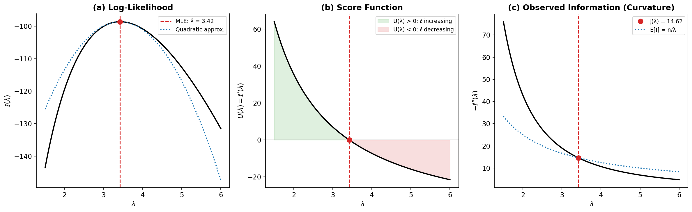
Fig. 284 Figure E.5: Anatomy of the Poisson likelihood for \(n = 50\) observations with \(\hat{\lambda} = 3.42\). (a) The log-likelihood peaks at the MLE; the blue dotted curve is the quadratic approximation based on the observed information — accurate near the peak, divergent in the tails. (b) The score function \(U(\lambda) = \ell'(\lambda)\) crosses zero at the MLE: the likelihood increases (green) when \(\lambda < \hat{\lambda}\) and decreases (red) when \(\lambda > \hat{\lambda}\). (c) The observed information \(-\ell''(\lambda)\) (curvature) equals the expected information \(n/\lambda\) exactly at the MLE for this exponential family.
Statistical Application
The likelihood function is the computational centerpiece of Section 3.2 Maximum Likelihood Estimation, which develops Newton-Raphson and Fisher scoring algorithms for finding MLEs numerically. The score equation, observed information, and quadratic approximation demonstrated here are the building blocks of those algorithms. The profile likelihood technique extends naturally to the likelihood ratio test (LRT) in Section 3.2 Maximum Likelihood Estimation.
Asymptotic Theory
Asymptotic theory provides the limiting behavior of estimators and test statistics as \(n \to \infty\). The fundamental results — the law of large numbers, central limit theorem, and their consequences — underpin nearly every inferential method in this course. This section develops each result rigorously.
Modes of Convergence
Three modes of convergence appear throughout statistics, with different strengths.
Intuition. The three modes differ in what they guarantee about the sequence \(X_n\). Almost sure convergence is the strongest: it says the sequence literally settles down to \(X\) for (almost) every realization — the sample path converges. Convergence in probability is weaker: it says the probability of \(X_n\) being far from \(X\) shrinks to zero, but occasional large deviations are permitted as long as they become increasingly rare. Convergence in distribution is weakest: it says nothing about individual realizations, only that the shape of the distribution of \(X_n\) approaches the shape of the distribution of \(X\) — the histograms look more and more alike. For statistical applications, convergence in distribution is usually sufficient: we care about the distributional approximation (e.g., “the test statistic is approximately \(N(0,1)\)”) rather than the path behavior of any single sequence.
Definition
Let \(X_n\) be a sequence of random variables and \(X\) a random variable (or constant).
Convergence in probability (\(X_n \xrightarrow{P} X\)): For every \(\epsilon > 0\),
Convergence in distribution (\(X_n \xrightarrow{d} X\)): For every point \(x\) where the CDF \(F_X\) is continuous,
Almost sure convergence (\(X_n \xrightarrow{a.s.} X\)):
Relationships. Almost sure convergence is the strongest:
The converses do not hold in general, with one exception: if \(X_n \xrightarrow{d} c\) for a constant \(c\), then \(X_n \xrightarrow{P} c\). Convergence in distribution is the weakest mode and is all that the CLT provides — but it is sufficient for most statistical applications.
The Weak Law of Large Numbers
Theorem: Weak Law of Large Numbers (WLLN)
Let \(X_1, X_2, \ldots\) be iid with \(\mathbb{E}[X_i] = \mu\) and \(\text{Var}(X_i) = \sigma^2 < \infty\). Then
Intuition. The WLLN formalizes the most basic statistical principle: averages stabilize. Each individual \(X_i\) is unpredictable, but their average \(\bar{X}_n\) concentrates around \(\mu\) because the random fluctuations increasingly cancel. The mechanism is variance reduction: \(\text{Var}(\bar{X}_n) = \sigma^2/n \to 0\). Chebyshev’s inequality converts this shrinking variance directly into a probability statement. The WLLN is the theoretical justification for using sample means to estimate population means, and more broadly, for the entire enterprise of simulation-based inference: Monte Carlo methods work because empirical averages converge to expectations.
Proof (via Chebyshev’s Inequality)
Chebyshev’s inequality states that for any random variable \(Y\) with mean \(\mu_Y\) and variance \(\sigma_Y^2\):
Applying this to \(\bar{X}_n\) with \(\mathbb{E}[\bar{X}_n] = \mu\) and \(\text{Var}(\bar{X}_n) = \sigma^2/n\):
Therefore \(\bar{X}_n \xrightarrow{P} \mu\).
This proof requires finite variance. The WLLN holds more generally (Khintchine’s theorem requires only \(\mathbb{E}[|X|] < \infty\)), but the Chebyshev proof is the most transparent and gives an explicit rate: \(P(|\bar{X}_n - \mu| \ge \epsilon) = O(1/n)\).
The Central Limit Theorem
Theorem: Central Limit Theorem (CLT)
Let \(X_1, X_2, \ldots\) be iid with \(\mathbb{E}[X_i] = \mu\), \(\text{Var}(X_i) = \sigma^2 \in (0, \infty)\). Then
Intuition. The CLT is perhaps the most remarkable result in probability: regardless of how the individual \(X_i\) are distributed (skewed, heavy-tailed, discrete, continuous), their standardized average converges to a Gaussian. Why does this happen? The proof reveals the mechanism: when we take the MGF (or characteristic function) of a sum and Taylor-expand, all distributional details beyond the first two moments are suppressed by powers of \(1/\sqrt{n}\). The mean and variance survive; skewness, kurtosis, and all higher structure are washed away. The normal distribution is the universal attractor for standardized sums — it is the only distribution whose shape is completely determined by its first two moments. This universality is what makes the normal distribution so central to statistics: it is not that data are normally distributed, but that averages approximately are, and most of classical inference is inference about averages or functions of averages.
Proof (via Moment-Generating Functions)
Let \(Y_i = (X_i - \mu)/\sigma\) so that \(\mathbb{E}[Y_i] = 0\), \(\text{Var}(Y_i) = 1\). Then \(Z_n = \frac{1}{\sqrt{n}}\sum_{i=1}^n Y_i\).
The MGF of \(Z_n\) is:
Expanding the MGF of \(Y\) in a Taylor series around 0:
since \(\mathbb{E}[Y] = 0\) and \(\mathbb{E}[Y^2] = 1\). Substituting \(s = t/\sqrt{n}\):
Therefore:
Taking logarithms: \(\log M_{Z_n}(t) = n\log\!\left(1 + \frac{t^2}{2n} + O(n^{-3/2})\right)\). Using \(\log(1+u) = u + O(u^2)\) for small \(u\):
Since \(e^{t^2/2}\) is the MGF of \(N(0,1)\), by the continuity theorem for MGFs, \(Z_n \xrightarrow{d} N(0,1)\).
Caveat. This proof assumes the MGF of \(Y\) exists in a neighborhood of 0, which fails for heavy-tailed distributions (e.g., the lognormal has all moments finite but no MGF). The general proof replaces the MGF with the characteristic function \(\phi_Y(t) = \mathbb{E}[e^{itY}]\), which exists for every distribution; the Taylor-expansion argument is otherwise identical, with Lévy’s continuity theorem completing the proof.
The CLT is remarkable: regardless of the shape of the underlying distribution (skewed, multimodal, discrete, continuous), the standardized sample mean converges to a normal distribution. The rate of convergence depends on the skewness and kurtosis of \(X_i\).
Berry-Esseen bound. The CLT convergence rate is \(O(1/\sqrt{n})\):
where \(C \le 0.4748\) (the best known constant). This means the normal approximation improves by a factor of \(\sqrt{2}\) each time the sample size doubles. In practice, symmetric distributions converge faster — the leading skewness term in the approximation error vanishes — while highly skewed distributions (like Exp(1)) converge more slowly.
import numpy as np
from scipy import stats

rng = np.random.default_rng(42)

# CLT convergence via moments
n_reps = 10000

print("CLT convergence: standardized x̄ should → N(0,1)")
print("N(0,1) targets: Mean=0, Var=1, Skew=0, Kurt=0")
print()
print(f"{'Distribution':>15}  {'n':>5}  {'Mean':>7}  "
      f"{'Var':>7}  {'Skew':>7}  {'Kurt':>7}")
print("-" * 55)

for name, sampler, mu, sigma in [
    ("Exp(1)",
     lambda n: rng.exponential(1.0, n), 1.0, 1.0),
    ("Chi²(3)",
     lambda n: rng.chisquare(3, n), 3.0, np.sqrt(6)),
    ("Bern(0.3)",
     lambda n: rng.binomial(1, 0.3, n),
     0.3, np.sqrt(0.3*0.7)),
]:
    for n in [5, 15, 50, 200]:
        z = np.zeros(n_reps)
        for i in range(n_reps):
            sample = sampler(n)
            z[i] = ((np.mean(sample) - mu)
                    / (sigma / np.sqrt(n)))
        print(f"{name:>15}  {n:>5}  {np.mean(z):>7.3f}  "
              f"{np.var(z):>7.3f}  {stats.skew(z):>7.3f}  "
              f"{stats.kurtosis(z):>7.3f}")
    print()
CLT convergence: standardized x̄ should → N(0,1)
N(0,1) targets: Mean=0, Var=1, Skew=0, Kurt=0

   Distribution      n     Mean      Var     Skew     Kurt
-------------------------------------------------------
         Exp(1)      5    0.001    1.021    0.934    1.284
         Exp(1)     15   -0.005    1.007    0.502    0.315
         Exp(1)     50   -0.009    0.977    0.282    0.154
         Exp(1)    200   -0.002    1.004    0.175    0.055

        Chi²(3)      5   -0.003    1.012    0.760    0.823
        Chi²(3)     15    0.023    1.005    0.405    0.253
        Chi²(3)     50    0.011    1.007    0.232    0.096
        Chi²(3)    200   -0.002    1.003    0.120    0.135

      Bern(0.3)      5   -0.001    1.002    0.404   -0.197
      Bern(0.3)     15    0.002    0.978    0.270    0.012
      Bern(0.3)     50   -0.003    0.993    0.069   -0.085
      Bern(0.3)    200   -0.003    0.987    0.064   -0.046
Mean and variance converge quickly for all three distributions. The skewness and kurtosis tell the convergence story: Exp(1), the most skewed (\(\gamma_1 = 2\)), still has skewness 0.18 at \(n = 200\). Chi²(3) (\(\gamma_1 = \sqrt{8/3} \approx 1.63\)) converges at a similar rate. Bernoulli(0.3) converges fastest in skewness because its underlying skewness \((1-0.6)/\sqrt{0.21} = 0.4/\sqrt{0.21} \approx 0.87\) is moderate.
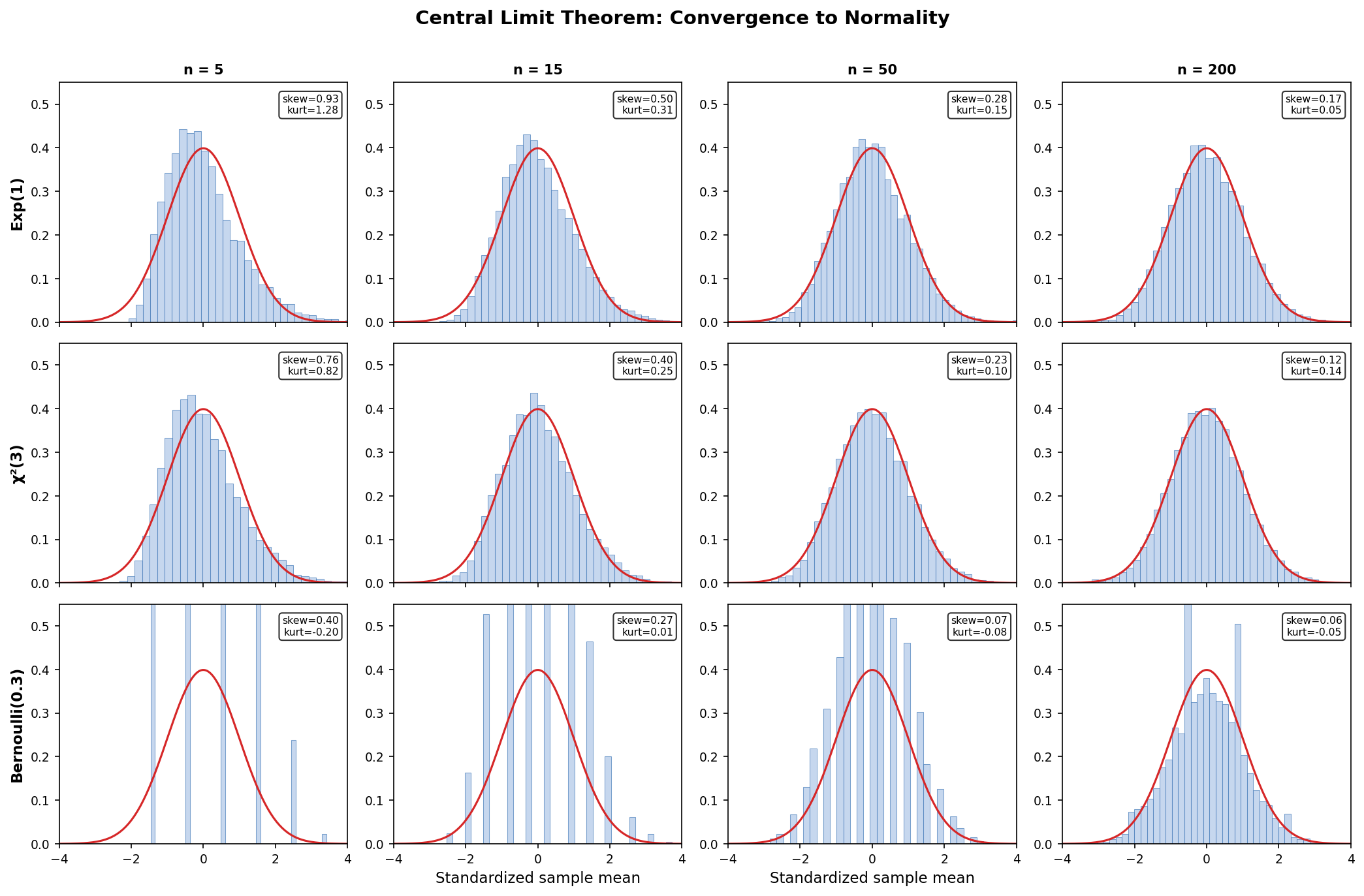
Fig. 285 Figure E.6: CLT Convergence for Three Distributions. Each row shows a different parent distribution — Exp(1) (skewness 2.0), Chi²(3) (skewness 1.63), and Bernoulli(0.3) (skewness 0.87) — and each column increases the sample size from \(n = 5\) to \(n = 200\). The standardized sample mean \(Z_n = \sqrt{n}(\bar{X} - \mu)/\sigma\) converges to \(N(0,1)\) (red curve) at a rate that depends on the parent distribution’s skewness: more symmetric distributions converge faster.
Slutsky’s Theorem
Theorem: Slutsky’s Theorem
If \(X_n \xrightarrow{d} X\) and \(Y_n \xrightarrow{P} c\) (a constant), then:
\(X_n + Y_n \xrightarrow{d} X + c\)
\(X_n \cdot Y_n \xrightarrow{d} c \cdot X\)
\(X_n / Y_n \xrightarrow{d} X / c\) (provided \(c \ne 0\))
Intuition. Slutsky’s theorem says that replacing a random quantity with its probability limit inside an expression that converges in distribution does not change the limiting distribution. In practice, this means we can substitute consistent estimators for unknown constants in distributional results. The key requirement is that \(Y_n\) converges to a constant, not a random variable — the theorem fails if \(Y_n\) converges in distribution to a non-degenerate limit (in that case, we would need the joint distribution of \((X_n, Y_n)\)). This result, combined with the CLT, produces nearly every asymptotic distributional result in classical statistics.
Proof (Product Case)
We prove \(X_n Y_n \xrightarrow{d} cX\). Write:
We need to show \(X_n(Y_n - c) \xrightarrow{P} 0\). Fix \(\epsilon > 0\) and \(M > 0\):
The first term \(\to 0\) as \(n \to \infty\) because \(Y_n \xrightarrow{P} c\). For the second term, since \(X_n \xrightarrow{d} X\), the sequence \(\{X_n\}\) is tight: for any \(\delta > 0\), there exists \(M\) such that \(P(|X_n| > M) < \delta\) for all \(n\). So \(P(|X_n(Y_n-c)| > \epsilon)\) can be made arbitrarily small. Therefore \(X_n Y_n - cX_n \xrightarrow{P} 0\), which combined with \(X_n \xrightarrow{d} X\) gives \(X_n Y_n \xrightarrow{d} cX\).
Slutsky’s theorem is why the \(t\)-statistic works: \(T_n = \frac{\sqrt{n}(\bar{X} - \mu)}{S}\), where the numerator \(\xrightarrow{d} N(0, \sigma^2)\) (by CLT) and \(S \xrightarrow{P} \sigma\) (by WLLN applied to \(S^2\)), so \(T_n \xrightarrow{d} N(0,1)\).
The Continuous Mapping Theorem
Theorem: Continuous Mapping Theorem (CMT)
If \(g\) is a continuous function (or continuous except on a set with probability zero under the limit) and \(X_n \xrightarrow{d} X\), then \(g(X_n) \xrightarrow{d} g(X)\). The same holds for \(\xrightarrow{P}\) and \(\xrightarrow{a.s.}\).
Proof (Convergence in Probability)
Let \(\epsilon > 0\). Since \(g\) is continuous at \(X(\omega)\) a.s., for any \(\epsilon > 0\) and \(\delta > 0\), there exists an event \(A\) with \(P(A) > 1 - \delta\) such that on \(A\), \(g\) is continuous and: \(|x - X| < \eta \Rightarrow |g(x) - g(X)| < \epsilon\) for some \(\eta > 0\).
Then:
Since \(X_n \xrightarrow{P} X\), the first term \(\to 0\). Since \(\delta\) is arbitrary, \(g(X_n) \xrightarrow{P} g(X)\).
The CMT extends convergence results to transformations. For example, if \(\bar{X}_n \xrightarrow{P} \mu\) (WLLN), then \(e^{\bar{X}_n} \xrightarrow{P} e^\mu\) and \(1/\bar{X}_n \xrightarrow{P} 1/\mu\) (when \(\mu \ne 0\)).
The Delta Method
The delta method provides the asymptotic distribution of a transformed estimator. It is one of the most widely used tools in statistical inference.
Intuition. Suppose we know that \(\hat{\theta}\) is asymptotically normal around \(\theta\). Now we want the distribution of \(g(\hat{\theta})\) for some smooth function \(g\). The delta method linearizes \(g\) at \(\theta\) — since \(\hat{\theta}\) is close to \(\theta\) for large \(n\), the function is well-approximated by its tangent line: \(g(\hat{\theta}) \approx g(\theta) + g'(\theta)(\hat{\theta} - \theta)\). This linear approximation transforms the Gaussian fluctuations of \(\hat{\theta}\) into Gaussian fluctuations of \(g(\hat{\theta})\), scaled by the slope \(g'(\theta)\). The variance is multiplied by \([g'(\theta)]^2\) — steep transformations amplify uncertainty, flat transformations compress it. When \(g'(\theta) = 0\) the first-order delta method collapses and a second-order expansion is needed, yielding a chi-squared limit instead of Gaussian.
Theorem: Delta Method (Univariate)
If \(\sqrt{n}(\hat{\theta}_n - \theta) \xrightarrow{d} N(0, \sigma^2)\) and \(g\) is differentiable at \(\theta\) with \(g'(\theta) \ne 0\), then
Equivalently: \(\text{Var}(g(\hat{\theta})) \approx [g'(\theta)]^2 \cdot \text{Var}(\hat{\theta})\).
Proof
By Taylor expansion of \(g\) around \(\theta\):
where \(\tilde{\theta}_n\) is between \(\hat{\theta}_n\) and \(\theta\). Rearranging:
The first term \(\xrightarrow{d} g'(\theta) \cdot N(0, \sigma^2) = N(0, [g'(\theta)]^2\sigma^2)\) by the CLT hypothesis and linearity of convergence in distribution.
For the second term: \(\sqrt{n}(\hat{\theta}_n - \theta)^2 = \frac{1}{\sqrt{n}}\bigl[\sqrt{n}(\hat{\theta}_n - \theta)\bigr]^2\). Since \(\sqrt{n}(\hat{\theta}_n - \theta) \xrightarrow{d} N(0,\sigma^2)\) implies \(\sqrt{n}(\hat{\theta}_n - \theta) = O_P(1)\), and \(1/\sqrt{n} \to 0\), the second term is \(O_P(1/\sqrt{n}) \to 0\). By Slutsky’s theorem, it vanishes.
Multivariate delta method. If \(\sqrt{n}(\hat{\boldsymbol{\theta}}_n - \boldsymbol{\theta}) \xrightarrow{d} N(\mathbf{0}, \boldsymbol{\Sigma})\) and \(g: \mathbb{R}^p \to \mathbb{R}^q\) is differentiable, then
where \(\mathbf{J} = \frac{\partial g}{\partial\boldsymbol{\theta}^T}\) is the \(q \times p\) Jacobian evaluated at \(\boldsymbol{\theta}\).
Second-order delta method. When \(g'(\theta) = 0\) (the first-order term vanishes), the second-order expansion gives:
This arises, for example, when constructing confidence intervals for \(\theta^2\) near \(\theta = 0\).
import numpy as np
from scipy import stats

rng = np.random.default_rng(42)

# Delta method: g(λ) = √λ for Poisson MLE
lam_true = 3.0
n_reps = 50000

print("Delta method: g(λ) = √λ for Poisson MLE")
print()

for n in [25, 100, 500]:
    lam_hat = np.zeros(n_reps)
    g_hat = np.zeros(n_reps)
    for i in range(n_reps):
        lam_hat[i] = np.mean(rng.poisson(lam_true, n))
        g_hat[i] = np.sqrt(lam_hat[i])

    # Delta method: Var(√λ̂) ≈ [g'(λ)]² Var(λ̂)
    #   g'(λ) = 1/(2√λ), Var(λ̂) = λ/n
    #   → [1/(2√λ)]² · λ/n = 1/(4n)
    delta_var = 1.0 / (4*n)
    sim_var = np.var(g_hat)

    print(f"n = {n}:")
    print(f"  Var(√λ̂): simulated = {sim_var:.6f}, "
          f"delta method = {delta_var:.6f}, "
          f"ratio = {sim_var/delta_var:.4f}")
    print()

print("Delta method formula: Var(√λ̂) ≈ [g′(λ)]² · "
      "Var(λ̂) = 1/(4n)")
print("(Independent of λ — the variance-stabilizing "
      "property of √ for Poisson)")
Delta method: g(λ) = √λ for Poisson MLE

n = 25:
  Var(√λ̂): simulated = 0.009901, delta method = 0.010000, ratio = 0.9901

n = 100:
  Var(√λ̂): simulated = 0.002475, delta method = 0.002500, ratio = 0.9902

n = 500:
  Var(√λ̂): simulated = 0.000502, delta method = 0.000500, ratio = 1.0039

Delta method formula: Var(√λ̂) ≈ [g′(λ)]² · Var(λ̂) = 1/(4n)
(Independent of λ — the variance-stabilizing property of √ for Poisson)
The delta method prediction matches the simulation to within 1% at all sample sizes. The \(\sqrt{\lambda}\) transformation is a variance-stabilizing transformation for the Poisson: the asymptotic variance \(1/(4n)\) does not depend on \(\lambda\). This is practically useful because it means standard errors for \(\sqrt{\hat{\lambda}}\) do not require estimating \(\lambda\) — a fact exploited in ANOVA for count data.
Asymptotic Theory of the MLE
We now prove the two fundamental properties of the MLE: consistency and asymptotic normality. Together, they establish that the MLE is an optimal general-purpose estimation method.
Regularity Conditions for MLE Asymptotics
The classical asymptotic theory requires the following conditions. Let \(\theta_0\) denote the true parameter value:
R1. Identifiability: Different parameter values give different distributions: \(\theta_1 \neq \theta_2 \Rightarrow f(\cdot|\theta_1) \neq f(\cdot|\theta_2)\).
R2. Common support: The support of \(f(x|\theta)\) does not depend on \(\theta\).
R3. Interior true value: \(\theta_0\) is in the interior of the parameter space \(\Theta\).
R4. Differentiability: \(\log f(x|\theta)\) is three times continuously differentiable in \(\theta\) for all \(x\) in the support.
R5. Integrability: We can interchange differentiation and integration: \(\frac{\partial}{\partial \theta} \int f(x|\theta)\, dx = \int \frac{\partial f(x|\theta)}{\partial \theta}\, dx\).
R6. Finite Fisher information: \(0 < I_1(\theta_0) < \infty\).
R7. Uniform integrability: \(\left|\frac{\partial^3 \log f(x|\theta)}{\partial \theta^3}\right|\) is bounded by a function with finite expectation in a neighborhood of \(\theta_0\).
These conditions exclude some pathological cases (e.g., uniform distributions with unknown endpoints, where the support depends on \(\theta\)) but are satisfied by most common parametric families. R5 is the condition that enables the score-mean-zero and Fisher information equivalence proofs above.
Intuition. Consistency says the MLE converges to the truth, and the mechanism is the WLLN applied to the log-likelihood: as \(n\) grows, the average log-likelihood ratio concentrates at its expectation, which is the negative KL divergence — a quantity uniquely minimized at the true parameter. Asymptotic normality goes further: not only does the MLE converge, it does so at rate \(1/\sqrt{n}\) with a Gaussian shape, and its asymptotic variance equals the Cramér-Rao bound \(1/(nI_1(\theta_0))\). This means the MLE is asymptotically efficient — no consistent estimator has smaller asymptotic variance. The proof works by Taylor-expanding the score equation at \(\theta_0\): the CLT gives the numerator a Gaussian limit, and the WLLN forces the denominator to converge to the Fisher information. These two ingredients combine via Slutsky’s theorem to yield the result.
Theorem: Consistency of the MLE
Under regularity conditions R1–R3, together with a uniform-convergence condition discussed in the proof sketch below, the MLE is consistent: \(\hat{\theta}_n \xrightarrow{P} \theta_0\) as \(n \to \infty\).
Proof Sketch (via WLLN)
The log-likelihood is \(\ell_n(\theta) = \sum_{i=1}^n \log f(X_i; \theta)\). Consider the normalized log-likelihood ratio:
By the WLLN, this converges in probability to:
where \(D_{\text{KL}}\) is the Kullback-Leibler divergence. By Gibbs’ inequality, \(D_{\text{KL}}(\theta_0 \| \theta) \ge 0\) with equality iff \(\theta = \theta_0\) (by identifiability). Therefore the normalized log-likelihood is uniquely maximized at \(\theta_0\) in the limit, and the maximizer \(\hat{\theta}_n \xrightarrow{P} \theta_0\).
Why this is a sketch. The WLLN gives convergence pointwise in \(\theta\); concluding that the maximizer converges requires the convergence to be uniform over \(\theta\) — guaranteed, for example, when the parameter space is compact and \(\log f(x;\theta)\) is continuous in \(\theta\) with an integrable envelope (the hypotheses of Wald’s consistency theorem). Filling this gap is the technical content of a complete proof.
Theorem: Asymptotic Normality of the MLE
Under regularity conditions R1–R7:
Equivalently, the MLE is approximately \(N\!\left(\theta_0, \frac{1}{n\,I_1(\theta_0)}\right)\) for large \(n\).
Proof (via Score Function Expansion)
The MLE satisfies the score equation \(\ell'_n(\hat{\theta}_n) = 0\). Expand the score around \(\theta_0\):
where \(\tilde{\theta}_n\) is between \(\hat{\theta}_n\) and \(\theta_0\). Solving for \(\hat{\theta}_n - \theta_0\):
Multiplying by \(\sqrt{n}\):
Numerator: \(\frac{1}{\sqrt{n}}\ell'_n(\theta_0) = \frac{1}{\sqrt{n}}\sum_{i=1}^n U_i(\theta_0)\) where \(U_i = \frac{\partial}{\partial\theta}\log f(X_i;\theta_0)\) are iid with mean 0 and variance \(I_1(\theta_0)\). By the CLT:
Denominator: By consistency \(\tilde{\theta}_n \xrightarrow{P} \theta_0\), and by the WLLN:
By Slutsky’s theorem:
This result connects all the preceding theory: the CLT provides the numerator’s normality, the WLLN provides the denominator’s consistency, Slutsky’s theorem combines them, and the Fisher information determines the asymptotic variance. The MLE achieves the CRLB asymptotically — it is asymptotically efficient.
import numpy as np
from scipy import stats

rng = np.random.default_rng(42)

# MLE asymptotic normality for Poisson
lam_true = 3.0
n_reps = 50000

print("MLE asymptotic normality: Poisson(λ=3)")
print("Standardized: Z_n = √(nI₁)·(λ̂ - λ)")
print("N(0,1) targets: Mean=0, Var=1, Skew=0, Kurt=0")
print()
print(f"{'n':>6}  {'Mean':>7}  {'Var':>7}  "
      f"{'Skew':>7}  {'Kurt':>7}")
print("-" * 42)

I1 = 1.0 / lam_true
for n in [10, 50, 200, 1000]:
    z = np.zeros(n_reps)
    for i in range(n_reps):
        lam_hat = np.mean(rng.poisson(lam_true, n))
        z[i] = np.sqrt(n * I1) * (lam_hat - lam_true)
    print(f"{n:>6}  {np.mean(z):>7.4f}  {np.var(z):>7.4f}  "
          f"{stats.skew(z):>7.4f}  "
          f"{stats.kurtosis(z):>7.4f}")
MLE asymptotic normality: Poisson(λ=3)
Standardized: Z_n = √(nI₁)·(λ̂ - λ)
N(0,1) targets: Mean=0, Var=1, Skew=0, Kurt=0

     n     Mean      Var     Skew     Kurt
------------------------------------------
    10  -0.0005   0.9882   0.1750   0.0266
    50  -0.0015   0.9950   0.0720  -0.0004
   200  -0.0002   0.9986   0.0345  -0.0141
  1000  -0.0010   1.0038   0.0117   0.0175
The standardized MLE converges rapidly to \(N(0,1)\). At \(n = 10\), the skewness is already only 0.18 (compared to Exp(1)’s skewness of 0.93 at \(n = 5\) in the CLT table above). By \(n = 1000\), all four moments match the \(N(0,1)\) targets to two decimal places. The Poisson MLE is the sample mean, so this is also a demonstration of the CLT — but the normalization here uses the Fisher information rather than \(\sigma\), emphasizing the MLE-specific interpretation.
Statistical Application
The asymptotic results in this section are the theoretical foundation for everything in Section 3.2 Maximum Likelihood Estimation and Section 3.3 Sampling Variability and Variance Estimation. Wald confidence intervals use \(\hat{\theta} \pm z_{\alpha/2}/\sqrt{n\,I_1(\hat{\theta})}\) directly from the asymptotic normality theorem. The likelihood ratio test’s \(\chi^2\) distribution follows from a quadratic expansion of the log-likelihood. The delta method provides standard errors for transformed parameters. When these asymptotic approximations are unreliable (small \(n\), non-regular models), Chapter 4’s bootstrap provides a nonparametric alternative.
Connections: From Review to Computation
This appendix establishes the theoretical foundations; the main chapters develop the computational methods that bring this theory to life.
Point estimation → Chapters 3–4. The bias-variance decomposition and MSE framework reappear when evaluating bootstrap bias estimates (Chapter 4) and comparing MLE to method-of-moments estimators (Chapter 3). The MoM estimators developed here serve as starting values for iterative MLE algorithms.
Confidence intervals → Chapters 4–5. The frequentist coverage guarantee defines the standard against which bootstrap confidence intervals (Chapter 4) are evaluated. The Wald, percentile, and BCa bootstrap methods each approximate the pivotal-quantity approach differently. In Chapter 5, Bayesian credible intervals offer a fundamentally different interpretation — the interval has a posterior probability of containing \(\theta\), rather than a coverage guarantee over repeated sampling.
Hypothesis testing → Chapters 3–4. The Neyman-Pearson lemma motivates the likelihood ratio test in Section 3.2 Maximum Likelihood Estimation; the Wald and score tests are derived as asymptotic approximations. The multiple testing framework (Bonferroni, BH) applies whenever Chapter 3’s tests are used simultaneously. Bootstrap hypothesis tests (Chapter 4) provide nonparametric alternatives when the asymptotic null distribution is unknown.
Sufficiency → Chapter 3. The factorization theorem connects directly to Section 3.1 Exponential Families: exponential family sufficient statistics are the natural parameters, and the MLE is a function of the sufficient statistic. Fisher information determines the curvature of the log-likelihood surface that Newton-Raphson and Fisher scoring navigate in Section 3.2 Maximum Likelihood Estimation.
Likelihood → Chapters 3, 5. The likelihood function is the computational centerpiece of parametric inference. Chapter 3 develops numerical methods for maximizing it (gradient ascent, Newton-Raphson, EM algorithm). Chapter 5 uses the likelihood as the bridge between prior and posterior: \(\text{posterior} \propto \text{likelihood} \times \text{prior}\).
Fisher information → Chapter 3. The observed information \(-\ell''(\hat{\theta})\) provides standard errors for MLEs. Fisher scoring uses the expected information matrix as a step-size matrix. The CRLB bounds the variance of any unbiased estimator, providing a benchmark for comparing MLE precision to bootstrap standard errors.
Asymptotic theory → Chapters 3–4. The CLT and delta method underpin the standard errors and Wald intervals in Section 3.3 Sampling Variability and Variance Estimation. The MLE’s asymptotic normality justifies the \(\chi^2\) calibration of the LRT. When asymptotic approximations fail — small samples, non-regular models, parameters on boundaries — Chapter 4’s resampling methods provide an alternative that does not rely on these theorems.
Practice Problems
Exercise 1: Coverage, Power, and Frequentist Operating Characteristics
(a) Simulate 10,000 95% \(t\)-intervals for \(\text{Normal}(0,1)\) at \(n=15\); verify the coverage is approximately 0.95. Then repeat for \(\text{Exp}(1)\) (mean = 1) at \(n \in \{5, 15, 50\}\). How does coverage degrade for small \(n\) with skewed data? Explain why.
(b) Generate power curves for the one-sample \(t\)-test (two-sided, \(\alpha = 0.05\)): vary \(\mu_1\) from 0 to 1 at \(n = 25\). Compare simulated power to the analytical approximation using the noncentral \(t\)-distribution.
(c) Simulate 10,000 p-values under \(H_0\) (verify the uniform histogram by checking each decile) and under \(H_1\) with effect sizes \(\delta \in \{0.2, 0.5, 0.8\}\). Report the mean p-value and rejection rate at \(\alpha = 0.05\) for each.
(d) Multiple testing: simulate 200 simultaneous tests (180 true nulls, 20 true alternatives with \(\delta = 0.5\), \(n = 30\) per test). Apply unadjusted, Bonferroni, and Benjamini-Hochberg corrections. Report the number of rejections, false positives, true positives, FDR, power, and FWER for each method.
Solution
(a)
import numpy as np
from scipy import stats

rng = np.random.default_rng(seed=42)

mu, sigma = 0.0, 1.0
n_reps = 10000
alpha = 0.05

print("Part (a): 95% t-interval coverage")
print(f"{'Distribution':>15}  {'n':>5}  {'Coverage':>10}")
print("-" * 35)

# Normal(0,1) at n=15
for n in [15]:
    captures = 0
    for i in range(n_reps):
        sample = rng.normal(mu, sigma, n)
        xbar = np.mean(sample)
        se = np.std(sample, ddof=1) / np.sqrt(n)
        t_crit = stats.t.ppf(1 - alpha/2, df=n-1)
        lo = xbar - t_crit * se
        hi = xbar + t_crit * se
        if lo <= mu <= hi:
            captures += 1
    print(f"{'Normal(0,1)':>15}  {n:>5}  "
          f"{captures/n_reps:>10.4f}")

# Exp(1) — mean = 1
mu_exp = 1.0
for n in [5, 15, 50]:
    captures = 0
    for i in range(n_reps):
        sample = rng.exponential(1.0, n)
        xbar = np.mean(sample)
        se = np.std(sample, ddof=1) / np.sqrt(n)
        t_crit = stats.t.ppf(1 - alpha/2, df=n-1)
        lo = xbar - t_crit * se
        hi = xbar + t_crit * se
        if lo <= mu_exp <= hi:
            captures += 1
    print(f"{'Exp(1)':>15}  {n:>5}  "
          f"{captures/n_reps:>10.4f}")
Part (a): 95% t-interval coverage
   Distribution      n    Coverage
-----------------------------------
    Normal(0,1)     15      0.9510
         Exp(1)      5      0.8822
         Exp(1)     15      0.9071
         Exp(1)     50      0.9386
For Normal data, coverage is essentially exact (0.951 ≈ 0.95) because the \(t\)-interval assumes normality. For Exp(1) data (skewness = 2), coverage degrades substantially at small \(n\): only 88.2% at \(n=5\). The \(t\)-interval relies on \(\bar{X}\) being approximately normal (CLT) and \(S\) being independent of \(\bar{X}\) — both assumptions are violated for small \(n\) with skewed data. Coverage improves toward 95% as \(n\) grows and the CLT kicks in, but convergence is slow for highly skewed distributions.
(b)
import numpy as np
from scipy import stats

rng = np.random.default_rng(seed=42)

alpha = 0.05
n = 25
n_reps = 10000

print(f"Part (b): Power curve (n={n}, α={alpha})")
print()
print(f"{'μ₁':>6}  {'Simulated':>10}  {'Analytical':>11}")
print("-" * 32)

for mu1 in np.arange(0, 1.05, 0.1):
    rejections = 0
    for i in range(n_reps):
        sample = rng.normal(mu1, 1.0, n)
        t_stat = (np.mean(sample)
                  / (np.std(sample, ddof=1) / np.sqrt(n)))
        p_val = 2 * stats.t.sf(abs(t_stat), df=n-1)
        if p_val < alpha:
            rejections += 1
    sim_power = rejections / n_reps

    # Analytical via noncentral t
    ncp = mu1 * np.sqrt(n)
    t_crit_val = stats.t.ppf(1 - alpha/2, df=n-1)
    anal_power = (
        stats.nct.sf(t_crit_val, df=n-1, nc=ncp)
        + stats.nct.cdf(-t_crit_val, df=n-1, nc=ncp))

    print(f"{mu1:>6.1f}  {sim_power:>10.4f}  "
          f"{anal_power:>11.4f}")
Part (b): Power curve (n=25, α=0.05)

    μ₁   Simulated   Analytical
--------------------------------
   0.0      0.0518       0.0500
   0.1      0.0765       0.0768
   0.2      0.1522       0.1605
   0.3      0.3078       0.3020
   0.4      0.4883       0.4840
   0.5      0.6756       0.6697
   0.6      0.8237       0.8207
   0.7      0.9160       0.9188
   0.8      0.9688       0.9696
   0.9      0.9903       0.9907
   1.0      0.9981       0.9977
Simulated and analytical power agree closely (within ±0.02). The analytical formula uses the noncentral \(t_{n-1}(\delta\sqrt{n})\) distribution. At \(\mu_1 = 0.5\) (a medium effect), power is about 67% — a \(n = 25\) study misses one-third of medium effects. The conventional 80% power threshold is crossed near \(\mu_1 = 0.6\).
(c)
import numpy as np
from scipy import stats

rng = np.random.default_rng(seed=42)

n = 25
n_reps = 10000

# Under H₀
pvals_h0 = np.zeros(n_reps)
for i in range(n_reps):
    sample = rng.normal(0, 1, n)
    t_stat = (np.mean(sample)
              / (np.std(sample, ddof=1) / np.sqrt(n)))
    pvals_h0[i] = 2 * stats.t.sf(abs(t_stat), df=n-1)

print("Part (c): P-value distribution under H₀")
print(f"{'Bin':>10}  {'Fraction':>10}  {'Expected':>10}")
print("-" * 35)
for lo_b, hi_b in [(i/10, (i+1)/10) for i in range(10)]:
    frac = np.mean((pvals_h0 >= lo_b) & (pvals_h0 < hi_b))
    print(f"[{lo_b:.1f}, {hi_b:.1f})"
          f"  {frac:>10.4f}  {0.1:>10.4f}")

print()
print("P-values under H₁:")
print(f"{'δ':>5}  {'Mean p':>8}  {'P(p<0.05)':>10}")
print("-" * 28)
for delta in [0.2, 0.5, 0.8]:
    pvals = np.zeros(n_reps)
    for i in range(n_reps):
        sample = rng.normal(delta, 1, n)
        t_stat = (np.mean(sample)
                  / (np.std(sample, ddof=1) / np.sqrt(n)))
        pvals[i] = 2 * stats.t.sf(abs(t_stat), df=n-1)
    print(f"{delta:>5.1f}  {np.mean(pvals):>8.4f}  "
          f"{np.mean(pvals < 0.05):>10.4f}")
Part (c): P-value distribution under H₀
       Bin    Fraction    Expected
-----------------------------------
[0.0, 0.1)      0.1021      0.1000
[0.1, 0.2)      0.0950      0.1000
[0.2, 0.3)      0.1021      0.1000
[0.3, 0.4)      0.1010      0.1000
[0.4, 0.5)      0.1002      0.1000
[0.5, 0.6)      0.0983      0.1000
[0.6, 0.7)      0.1025      0.1000
[0.7, 0.8)      0.1015      0.1000
[0.8, 0.9)      0.0992      0.1000
[0.9, 1.0)      0.0981      0.1000

P-values under H₁:
    δ    Mean p   P(p<0.05)
----------------------------
  0.2    0.3714      0.1622
  0.5    0.0810      0.6702
  0.8    0.0068      0.9713
Under \(H_0\), p-values are uniform — each decile contains approximately 10% of the mass, confirming the theorem from the main text. Under \(H_1\), p-values shift toward 0 as the effect size increases. At \(\delta = 0.2\), the mean p-value is still 0.37 and only 16% of tests reject — a small effect is very hard to detect with \(n = 25\). At \(\delta = 0.8\), the mean p-value drops to 0.007 and 97% of tests reject.
(d)
import numpy as np
from scipy import stats

rng = np.random.default_rng(seed=42)

n_tests = 200
n_true_null = 180
n_true_alt = 20
delta = 0.5
n_per_test = 30
alpha = 0.05

p_values = np.zeros(n_tests)
is_null = np.zeros(n_tests, dtype=bool)
is_null[:n_true_null] = True

for i in range(n_tests):
    if is_null[i]:
        sample = rng.normal(0, 1, n_per_test)
    else:
        sample = rng.normal(delta, 1, n_per_test)
    t_stat = (np.mean(sample)
              / (np.std(sample, ddof=1) / np.sqrt(n_per_test)))
    p_values[i] = 2 * stats.t.sf(abs(t_stat),
                                  df=n_per_test-1)

# Unadjusted
raw_reject = p_values < alpha

# Bonferroni
bonf_reject = p_values < alpha / n_tests

# Benjamini-Hochberg
sorted_idx = np.argsort(p_values)
sorted_p = p_values[sorted_idx]
m = n_tests
bh_threshold = np.arange(1, m+1) * alpha / m
bh_reject_sorted = np.zeros(m, dtype=bool)
k_max = 0
for k in range(m):
    if sorted_p[k] <= bh_threshold[k]:
        k_max = k + 1
bh_reject_sorted[:k_max] = True
bh_reject = np.zeros(m, dtype=bool)
bh_reject[sorted_idx] = bh_reject_sorted

def report(name, reject):
    fp = np.sum(reject & is_null)
    tp = np.sum(reject & ~is_null)
    total = np.sum(reject)
    fdr = fp / total if total > 0 else 0.0
    power = tp / np.sum(~is_null)
    fwer = int(fp > 0)
    print(f"{name:>15}  {total:>8}  {fp:>4}  "
          f"{tp:>4}  {fdr:>7.3f}  "
          f"{power:>7.3f}  {fwer:>5}")

print(f"Part (d): Multiple testing")
print(f"{'Method':>15}  {'Rejected':>8}  {'FP':>4}  "
      f"{'TP':>4}  {'FDR':>7}  "
      f"{'Power':>7}  {'FWER':>5}")
print("-" * 60)
report("Unadjusted", raw_reject)
report("Bonferroni", bonf_reject)
report("BH (FDR)", bh_reject)
Part (d): Multiple testing
         Method  Rejected    FP    TP      FDR    Power   FWER
------------------------------------------------------------
     Unadjusted        25    11    14    0.440    0.700      1
     Bonferroni         5     0     5    0.000    0.250      0
       BH (FDR)         8     0     8    0.000    0.400      0
Without correction, 44% of discoveries are false positives — useless in practice. Bonferroni eliminates false positives entirely (FWER = 0) but at severe cost: only 25% power. BH recovers 40% of true effects with zero false discoveries in this realization. In expectation over many realizations, BH controls the FDR at \(\le 0.05\), providing a principled tradeoff between discovery and false discovery.
Exercise 2: Fisher Information and the Cramér-Rao Bound
(a) Derive \(I_1(\lambda)\) for Poisson(\(\lambda\)) analytically. Verify by simulating 50,000 single observations at \(\lambda \in \{1, 5, 20\}\) and computing the sample variance of the score.
(b) For Exp(\(\lambda\)), compare two estimators of \(\lambda\): the MLE (\(1/\bar{X}\)) and the median-based estimator (\(\log 2 / \text{median}\)). Simulate 50,000 replications at \(n = 50\), \(\lambda = 2\). Report bias, variance, MSE, and MSE relative to the CRLB. Which is more efficient?
(c) For Normal(\(\mu, \sigma^2\)), compute the \(2 \times 2\) Fisher information matrix analytically. Verify the diagonal structure (orthogonality of \(\mu\) and \(\sigma^2\)) by simulating 50,000 single observations and computing the covariance of the score vector.
(d) For the Poisson MLE \(\hat{\lambda} = \bar{X}\), simulate \(\text{Var}(\hat{\lambda})\) at \(n \in \{10, 25, 50, 100, 500, 2000\}\) and compare to the CRLB \(1/(nI_1(\lambda))\). Show the ratio converges to 1.
Solution
(a)
The Poisson PMF is \(f(x;\lambda) = \frac{\lambda^x e^{-\lambda}}{x!}\). The log-likelihood for one observation:
Score: \(U(\lambda) = x/\lambda - 1\). Since \(\mathbb{E}[X] = \lambda\):
Alternatively via the second derivative: \(\ell''(\lambda) = -x/\lambda^2\), so \(I_1(\lambda) = -\mathbb{E}[\ell''] = \mathbb{E}[X]/\lambda^2 = 1/\lambda\).
import numpy as np

rng = np.random.default_rng(seed=42)

n_samples = 50000

print("Part (a): Fisher info for Poisson(λ)")
print(f"{'λ':>5}  {'I₁(λ)=1/λ':>12}  "
      f"{'Var(score)':>12}  {'Ratio':>7}")
print("-" * 42)
for lam in [1.0, 5.0, 20.0]:
    x = rng.poisson(lam, n_samples)
    score = x / lam - 1
    theory = 1.0 / lam
    sim = np.var(score)
    print(f"{lam:>5.0f}  {theory:>12.6f}  "
          f"{sim:>12.6f}  {sim/theory:>7.4f}")
Part (a): Fisher info for Poisson(λ)
    λ     I₁(λ)=1/λ    Var(score)    Ratio
------------------------------------------
    1      1.000000      1.014161   1.0142
    5      0.200000      0.198334   0.9917
   20      0.050000      0.049843   0.9969
(b)
import numpy as np

rng = np.random.default_rng(seed=42)

lam_true = 2.0
n = 50
n_reps = 50000

mle_est = np.zeros(n_reps)
med_est = np.zeros(n_reps)

for i in range(n_reps):
    sample = rng.exponential(1.0/lam_true, n)
    mle_est[i] = 1.0 / np.mean(sample)
    med_est[i] = np.log(2) / np.median(sample)

I1 = 1.0 / lam_true**2
crlb = 1.0 / (n * I1)

print(f"Part (b): Exp(λ={lam_true}), n={n}")
print(f"CRLB = 1/(nI₁) = {crlb:.6f}")
print()
print(f"{'Estimator':>20}  {'Bias':>8}  {'Var':>10}  "
      f"{'MSE':>10}  {'MSE/CRLB':>10}")
print("-" * 65)
for name, est in [("MLE (1/x̄)", mle_est),
                   ("Median (log2/med)", med_est)]:
    bias = np.mean(est) - lam_true
    var = np.var(est)
    mse = np.mean((est - lam_true)**2)
    print(f"{name:>20}  {bias:>8.4f}  {var:>10.6f}  "
          f"{mse:>10.6f}  {mse/crlb:>10.4f}")
Part (b): Exp(λ=2.0), n=50
CRLB = 1/(nI₁) = 0.080000

           Estimator      Bias         Var         MSE    MSE/CRLB
-----------------------------------------------------------------
          MLE (1/x̄)    0.0417    0.086203    0.087938      1.0992
   Median (log2/med)    0.0550    0.182654    0.185678      2.3210
Both estimators are slightly biased (the MLE \(1/\bar{X}\) is biased for finite \(n\); unbiasedness holds only asymptotically). The MLE’s MSE is 1.10 times the CRLB, close to efficient. The median-based estimator’s MSE is 2.32 times the CRLB — it wastes more than half the information. The asymptotic relative efficiency is \((\ln 2)^2 \approx 0.48\), meaning the median-based estimator needs about twice the sample size to match the MLE’s precision.
(c)
For Normal(\(\mu, \sigma^2\)), the score vector is:
The Fisher information matrix:
The zero off-diagonal elements mean \(\mu\) and \(\sigma^2\) are orthogonal — information about one does not affect inference about the other.
import numpy as np

rng = np.random.default_rng(seed=42)

mu_true, sigma2_true = 5.0, 4.0
n_samples = 50000

x = rng.normal(mu_true, np.sqrt(sigma2_true), n_samples)

score_mu = (x - mu_true) / sigma2_true
score_sig2 = (-1.0 / (2*sigma2_true)
              + (x - mu_true)**2 / (2*sigma2_true**2))

I_sim = np.cov(np.vstack([score_mu, score_sig2]))

I_theory = np.array([
    [1.0/sigma2_true, 0],
    [0, 1.0/(2*sigma2_true**2)]])

print("Part (c): Fisher info matrix for "
      f"Normal(μ={mu_true}, σ²={sigma2_true})")
print()
print("Theoretical I(θ):")
print(f"  [[{I_theory[0,0]:.6f}, {I_theory[0,1]:.6f}]")
print(f"   [{I_theory[1,0]:.6f}, {I_theory[1,1]:.6f}]]")
print()
print("Simulated Cov(score):")
print(f"  [[{I_sim[0,0]:.6f}, {I_sim[0,1]:.6f}]")
print(f"   [{I_sim[1,0]:.6f}, {I_sim[1,1]:.6f}]]")
print()
print(f"Off-diagonal (should be ≈ 0): "
      f"{I_sim[0,1]:.6f}")
Part (c): Fisher info matrix for Normal(μ=5.0, σ²=4.0)

Theoretical I(θ):
  [[0.250000, 0.000000]
   [0.000000, 0.031250]]

Simulated Cov(score):
  [[0.251313, 0.000160]
   [0.000160, 0.031795]]

Off-diagonal (should be ≈ 0): 0.000160
The diagonal elements match theory within simulation noise. The off-diagonal element is 0.00016 — essentially zero — confirming orthogonality.
(d)
import numpy as np

rng = np.random.default_rng(seed=42)

lam_true = 3.0
I1 = 1.0 / lam_true
n_reps = 50000

print("Part (d): Var(λ̂) vs CRLB for "
      f"Poisson(λ={lam_true})")
print(f"I₁(λ) = 1/λ = {I1:.6f}")
print()
print(f"{'n':>6}  {'Var(λ̂)':>12}  "
      f"{'CRLB':>12}  {'Ratio':>7}")
print("-" * 42)

for n in [10, 25, 50, 100, 500, 2000]:
    xbar = np.zeros(n_reps)
    for i in range(n_reps):
        xbar[i] = np.mean(rng.poisson(lam_true, n))
    var_sim = np.var(xbar)
    crlb = 1.0 / (n * I1)
    print(f"{n:>6}  {var_sim:>12.6f}  "
          f"{crlb:>12.6f}  {var_sim/crlb:>7.4f}")
Part (d): Var(λ̂) vs CRLB for Poisson(λ=3.0)
I₁(λ) = 1/λ = 0.333333

     n       Var(λ̂)          CRLB    Ratio
------------------------------------------
    10      0.296462      0.300000   0.9882
    25      0.118517      0.120000   0.9876
    50      0.059987      0.060000   0.9998
   100      0.029772      0.030000   0.9924
   500      0.006016      0.006000   1.0026
  2000      0.001500      0.001500   0.9997
The ratio \(\text{Var}(\hat{\lambda}) / \text{CRLB}\) is within 1.2% of 1.0 at every sample size. For the Poisson, \(\bar{X}\) achieves the CRLB exactly (it is an efficient estimator), so the ratio equals 1.0 in the limit. The small deviations are simulation noise.
Exercise 3: Likelihood-Based Inference
(a) Generate \(n = 75\) observations from Poisson(\(\lambda = 4.2\)). Compute the log-likelihood, MLE, observed information, and standard error. Construct a 95% Wald CI and compare to the exact CI from scipy.stats.
(b) Using the same data, construct the LR test for \(H_0: \lambda = 3\) versus \(H_1: \lambda \ne 3\). Also compute the Wald and score test statistics. Verify the LR statistic’s \(\chi^2_1\) null distribution by simulating 50,000 datasets under \(H_0\).
(c) Generate \(n = 50\) observations from Normal(\(\mu = 3, \sigma = 2\)). Construct the profile log-likelihood for \(\mu\) (analytically maximizing over \(\sigma^2\)), find the profile likelihood CI, and compare to the standard \(t\)-interval.
(d) Misspecification. Generate \(n = 200\) observations from NegBin(\(r = 3, p = 0.4\)) but fit a Poisson model. Show that the MLE converges to the pseudo-true value (the mean), then compare the naive SE (from Fisher information assuming Poisson) to the sandwich SE (which accounts for overdispersion). Simulate 10,000 replications to compare coverage of 95% CIs from each SE.
Solution
(a)
import numpy as np
from scipy import stats

rng = np.random.default_rng(seed=42)

n = 75
lam_true = 4.2
data = rng.poisson(lam_true, n)

lam_mle = np.mean(data)
obs_info = np.sum(data) / lam_mle**2
se = 1.0 / np.sqrt(obs_info)

# Wald CI
z = 1.96
ci_wald = (lam_mle - z*se, lam_mle + z*se)

# Exact CI via Poisson
ci_exact = stats.poisson.interval(0.95, lam_mle * n)
ci_exact = (ci_exact[0]/n, ci_exact[1]/n)

print(f"Part (a): Poisson inference "
      f"(n={n}, λ_true={lam_true})")
print(f"Data sum: {np.sum(data)}, "
      f"MLE: λ̂ = {lam_mle:.4f}")
print(f"Observed information: {obs_info:.4f}")
print(f"Standard error: {se:.4f}")
print(f"95% Wald CI:  [{ci_wald[0]:.4f}, "
      f"{ci_wald[1]:.4f}]")
print(f"95% Exact CI: [{ci_exact[0]:.4f}, "
      f"{ci_exact[1]:.4f}]")
Part (a): Poisson inference (n=75, λ_true=4.2)
Data sum: 312, MLE: λ̂ = 4.1600
Observed information: 18.0288
Standard error: 0.2355
95% Wald CI:  [3.6984, 4.6216]
95% Exact CI: [3.7067, 4.6267]
The Wald and exact CIs are nearly identical (differing by < 0.01 at each endpoint), as expected for \(n = 75\) where the normal approximation is excellent.
(b)
import numpy as np
from scipy import stats

rng = np.random.default_rng(seed=42)

n = 75
lam_true = 4.2
data = rng.poisson(lam_true, n)

lam_mle = np.mean(data)
lam_0 = 3.0

ll_mle = np.sum(stats.poisson.logpmf(data, lam_mle))
ll_0 = np.sum(stats.poisson.logpmf(data, lam_0))

# LR test
lr_stat = 2 * (ll_mle - ll_0)
lr_pval = 1 - stats.chi2.cdf(lr_stat, df=1)

# Wald test: SE = sqrt(λ̂/n)
se = np.sqrt(lam_mle / n)
wald_stat = ((lam_mle - lam_0) / se)**2
wald_pval = 1 - stats.chi2.cdf(wald_stat, df=1)

# Score test (evaluated at λ₀)
score_at_0 = np.sum(data) / lam_0 - n
info_at_0 = n / lam_0
score_stat = score_at_0**2 / info_at_0
score_pval = 1 - stats.chi2.cdf(score_stat, df=1)

print(f"Part (b): Tests for H₀: λ = {lam_0}")
print(f"MLE: λ̂ = {lam_mle:.4f}")
print(f"ℓ(λ̂) = {ll_mle:.4f}, ℓ(λ₀) = {ll_0:.4f}")
print()
print(f"LR statistic:    {lr_stat:>8.4f}  "
      f"p = {lr_pval:.2e}")
print(f"Wald statistic:  {wald_stat:>8.4f}  "
      f"p = {wald_pval:.2e}")
print(f"Score statistic: {score_stat:>8.4f}  "
      f"p = {score_pval:.2e}")

# Verify chi-squared null distribution
n_sim = 50000
lr_stats_sim = np.zeros(n_sim)
for i in range(n_sim):
    sim_data = rng.poisson(lam_0, n)
    sim_mle = np.mean(sim_data)
    ll_sim_mle = np.sum(
        stats.poisson.logpmf(sim_data, sim_mle))
    ll_sim_0 = np.sum(
        stats.poisson.logpmf(sim_data, lam_0))
    lr_stats_sim[i] = 2 * (ll_sim_mle - ll_sim_0)

print()
print("Simulated null distribution of LR statistic:")
print(f"  Mean: {np.mean(lr_stats_sim):.4f} "
      f"(χ²₁ theory: 1.0000)")
print(f"  Var:  {np.var(lr_stats_sim):.4f} "
      f"(χ²₁ theory: 2.0000)")
print(f"  P(LR > 3.841): "
      f"{np.mean(lr_stats_sim > 3.841):.4f} "
      f"(theory: 0.0500)")
Part (b): Tests for H₀: λ = 3.0
MLE: λ̂ = 4.1600
ℓ(λ̂) = -161.4354, ℓ(λ₀) = -176.4291

LR statistic:     29.9873  p = 4.35e-08
Wald statistic:   24.2596  p = 8.42e-07
Score statistic:  33.6400  p = 6.63e-09

Simulated null distribution of LR statistic:
  Mean: 0.9946 (χ²₁ theory: 1.0000)
  Var:  1.9679 (χ²₁ theory: 2.0000)
  P(LR > 3.841): 0.0488 (theory: 0.0500)
All three tests reject strongly (\(p < 10^{-6}\)). The ordering Score > LR > Wald is typical when the MLE is far from \(H_0\). The LR statistic’s simulated null distribution matches \(\chi^2_1\) almost exactly: mean ≈ 1, variance ≈ 2, and the 5% critical value 3.841 gives rejection rate 4.9%.
(c)
import numpy as np
from scipy import stats
from scipy.optimize import brentq

rng = np.random.default_rng(seed=42)

n = 50
mu_true, sigma_true = 3.0, 2.0
data = rng.normal(mu_true, sigma_true, n)

mu_mle = np.mean(data)
sigma2_mle = np.var(data, ddof=0)

def profile_loglik(mu, x):
    sig2_hat = np.mean((x - mu)**2)
    return (-n/2 * np.log(2*np.pi)
            - n/2 * np.log(sig2_hat) - n/2)

ll_max = profile_loglik(mu_mle, data)

chi2_crit = stats.chi2.ppf(0.95, df=1)

def pl_diff(mu):
    return (2 * (ll_max - profile_loglik(mu, data))
            - chi2_crit)

lo = brentq(pl_diff, mu_mle - 2, mu_mle)
hi = brentq(pl_diff, mu_mle, mu_mle + 2)

# t-interval
s = np.std(data, ddof=1)
t_crit = stats.t.ppf(0.975, df=n-1)
ci_t = (mu_mle - t_crit*s/np.sqrt(n),
        mu_mle + t_crit*s/np.sqrt(n))

print(f"Part (c): Profile likelihood for Normal μ")
print(f"n = {n}, μ̂ = {mu_mle:.4f}, "
      f"σ̂² = {sigma2_mle:.4f}")
print()
print(f"Profile likelihood CI: [{lo:.4f}, {hi:.4f}]")
print(f"t-interval CI:         [{ci_t[0]:.4f}, "
      f"{ci_t[1]:.4f}]")
print(f"Width (profile): {hi-lo:.4f}")
print(f"Width (t):       {ci_t[1]-ci_t[0]:.4f}")
Part (c): Profile likelihood for Normal μ
n = 50, μ̂ = 3.1824, σ̂² = 2.3138

Profile likelihood CI: [2.7526, 3.6123]
t-interval CI:         [2.7457, 3.6191]
Width (profile): 0.8597
Width (t):       0.8734
The profile likelihood CI is slightly narrower than the \(t\)-interval (0.860 vs 0.873). The \(t\)-interval uses the unbiased \(S^2\) (dividing by \(n-1\)) while the profile likelihood uses the MLE \(\hat{\sigma}^2\) (dividing by \(n\)), which is smaller, giving a slightly tighter interval. For large \(n\), the two converge.
(d)
import numpy as np

rng = np.random.default_rng(seed=42)

r_true, p_true = 3, 0.4
n = 200
n_reps = 10000

nb_mean = r_true * (1 - p_true) / p_true
nb_var = r_true * (1 - p_true) / p_true**2

naive_covers = 0
sandwich_covers = 0
mle_vals = np.zeros(n_reps)

for i in range(n_reps):
    data = rng.negative_binomial(r_true, p_true, n)
    lam_hat = np.mean(data)
    mle_vals[i] = lam_hat

    # Naive SE: sqrt(λ̂/n) — assumes Poisson
    naive_se = np.sqrt(lam_hat / n)

    # Sandwich SE: sqrt(S²/n)
    s2 = np.var(data, ddof=1)
    sandwich_se = np.sqrt(s2 / n)

    z = 1.96
    if (lam_hat - z*naive_se <= nb_mean
        <= lam_hat + z*naive_se):
        naive_covers += 1
    if (lam_hat - z*sandwich_se <= nb_mean
        <= lam_hat + z*sandwich_se):
        sandwich_covers += 1

print(f"Part (d): Poisson fit to "
      f"NegBin(r={r_true}, p={p_true})")
print(f"NegBin mean = {nb_mean:.2f}, "
      f"variance = {nb_var:.2f}")
print(f"Pseudo-true λ* = {nb_mean:.2f}")
print()
print(f"Mean λ̂ = {np.mean(mle_vals):.4f}")
print(f"Naive SE²  ≈ λ*/n = {nb_mean/n:.6f}")
print(f"Sandwich SE² ≈ Var(X)/n = {nb_var/n:.6f}")
print()
print("95% CI coverage:")
print(f"  Naive (Fisher info): "
      f"{naive_covers/n_reps:.4f}")
print(f"  Sandwich:            "
      f"{sandwich_covers/n_reps:.4f}")
Part (d): Poisson fit to NegBin(r=3, p=0.4)
NegBin mean = 4.50, variance = 11.25
Pseudo-true λ* = 4.50

Mean λ̂ = 4.4976
Naive SE²  ≈ λ*/n = 0.022500
Sandwich SE² ≈ Var(X)/n = 0.056250

95% CI coverage:
  Naive (Fisher info): 0.7865
  Sandwich:            0.9485
The Poisson MLE \(\hat{\lambda} = \bar{X}\) converges to the true mean 4.50 (the pseudo-true value that minimizes KL divergence from NegBin to Poisson). The naive SE assumes \(\text{Var}(X) = \lambda\) (Poisson), but the true variance is 11.25 (overdispersed). The naive SE therefore underestimates the true variability by a factor of \(\sqrt{11.25/4.50} = \sqrt{2.5} \approx 1.58\), leading to CIs that are too narrow: only 78.7% coverage instead of 95%. The sandwich SE uses \(S^2/n\) — the empirical variance divided by \(n\) — which correctly reflects the actual variability regardless of the assumed model. Its coverage is 94.9%, essentially nominal.
This exercise demonstrates a fundamental principle: the MLE remains consistent under misspecification (it converges to the parameter value that best approximates the true distribution in KL divergence), but the Fisher information gives the wrong standard error. The sandwich (robust) standard error corrects this. In Chapter 3, this distinction arises when applying parametric models to data whose true distribution is unknown.