Section 5.1 Foundations of Bayesian Inference
In Chapters 2 through 4 we built the frequentist computational toolkit piece by piece: Monte Carlo integration for approximating expectations, maximum likelihood for extracting information from parametric models, and resampling for quantifying the variability of estimators without analytical formulae. Every one of those methods answered questions about procedures — how an estimator behaves across hypothetical repetitions of an experiment, how a confidence interval performs in the long run, how a test’s Type I error rate is controlled. None of them answered what is arguably the most natural question a scientist or decision-maker can ask: Given the data I actually observed and whatever I already know, what should I believe about the unknown quantities that generated those data?
That question — a question about belief rather than procedure — is the province of Bayesian inference. We encountered the Bayesian paradigm in Section 1.1 Paradigms of Probability and Statistical Inference, where we compared its philosophical foundations with the frequentist and likelihood-based alternatives. We saw conjugate priors for exponential families in Section 3.1 Exponential Families, and Section 3.6 Chapter 3 Summary explicitly noted that “Chapter 5 presents the Bayesian alternative to maximum likelihood.” Now we make good on that promise. This section operationalizes the Bayesian framework: we move from philosophical comparison to mechanical application, developing the computational machinery that turns Bayes’ theorem from a mathematical identity into a practical inference engine.
The motivating problem is concrete. Suppose a pharmaceutical company runs a clinical trial of a new vaccine on \(n = 50\) volunteers and observes \(k = 38\) successes (immune response). What can be said about the true efficacy rate \(\theta\)? A frequentist constructs a confidence interval around the MLE \(\hat{\theta} = 38/50 = 0.76\). A Bayesian starts with a prior distribution on \(\theta\), updates it with the observed data, and obtains a posterior distribution — a complete probability distribution over all possible values of \(\theta\). Point estimates, interval estimates, predictions, and model comparisons all flow from this single posterior object.
Terminology note 📌
In clinical trial and regulatory language, efficacy has a specific technical meaning: it is a two-arm comparison (two groups of participants: one receives the treatment, the other serves as control), usually expressed as a relative risk reduction
which cannot be estimated from a single arm. The parameter \(\theta\) in the running example is actually the response rate in the treated group — the probability that a single vaccinated volunteer shows an immune response. We use “efficacy rate” informally throughout this chapter because the framing is familiar from public discussion of vaccine trials, but a true efficacy analysis would model the ratio (or difference) of two Binomial parameters, one per arm. The single-arm simplification keeps the focus on Bayesian machinery; the two-arm extension is a direct application of the same methods and appears in the exercises.
Road Map 🧭
Understand: The three-step Bayesian workflow (model specification → posterior computation → model evaluation) and how it contrasts with the frequentist pipeline from Chapter 3
Develop: Facility in mechanically applying Bayes’ theorem to both discrete and continuous parameter problems, including the proportional-to form that avoids the normalizing constant
Implement: Python functions for posterior computation via grid approximation and analytical conjugate formulas
Evaluate: When Bayesian analysis offers genuine advantages over frequentist alternatives, and the computational cost of those advantages
Historical Development: From Bayes’ Essay to the MCMC Revolution
The history of Bayesian inference is one of the most dramatic stories in the history of science — a method proposed in 1763, developed into a comprehensive framework by 1820, then nearly extinguished by the frequentist revolution of the early twentieth century, before being revived and ultimately triumphant thanks to a computational breakthrough in the 1990s. Understanding this trajectory is not mere historical curiosity: it explains why Bayesian methods were unavailable to the statisticians who built the frequentist framework you learned in Chapters 3–4, why the computational methods we develop in Sections 5.4–5.6 were so transformative, and why the philosophical debates from Section 1.1 Paradigms of Probability and Statistical Inference mattered so intensely for two centuries.
Bayes’ Essay and Laplace’s Synthesis
The story begins with the Reverend Thomas Bayes, a Presbyterian minister and amateur mathematician in Tunbridge Wells, England. Bayes was interested in a question that seems almost mundane today: if we observe the outcomes of several trials of an experiment, what can we infer about the probability of success on any individual trial? He formulated this as what we now call the Beta-Binomial problem — exactly the problem we will work through computationally later in this section.
Bayes never published his solution. After his death in 1761, his friend Richard Price found the manuscript among his papers, edited it, and submitted it to the Royal Society. The result — “An Essay towards Solving a Problem in the Doctrine of Chances” — appeared in 1763. Bayes’ key insight was to treat the unknown probability \(\theta\) not as a fixed constant but as a quantity about which we could reason probabilistically. He assumed a uniform prior — \(\theta\) equally likely to be anywhere in \([0,1]\) — and showed how to compute what we would now call the posterior distribution. The mathematical content of the essay is sound, if somewhat awkwardly expressed in the notation of the time, and includes what amounts to the first computation of a Beta posterior.
But it was Pierre-Simon Laplace who transformed Bayes’ particular result into a general methodology. Working independently and apparently unaware of Bayes’ essay until later, Laplace derived Bayes’ theorem in full generality in 1774 and spent the next four decades developing its consequences. His Théorie analytique des probabilités (1812) and the more accessible Essai philosophique sur les probabilités (1814) laid out a comprehensive program: probability is a measure of rational belief, Bayes’ theorem is the mechanism for updating belief in light of evidence, and the resulting posterior distribution is the basis for all inference.
Laplace applied this framework to an extraordinary range of problems: estimating the masses of planets, determining the orbits of comets, analyzing birth ratios (the famous question of whether boys are born more often than girls), correcting measurements for instrumental error, and predicting the probability of the sun rising tomorrow. For Laplace, Bayesian inference was not one approach among several — it was the only rational way to reason from data. The “probability of causes,” as he called the posterior distribution, was the complete answer to any scientific question. His famous dictum captures the Laplacian vision: “Probability theory is nothing but common sense reduced to calculation.”
For nearly a century after Laplace, what we now call Bayesian methods were simply “probability.” There was no alternative paradigm to contrast them with. Statisticians used inverse probability — reasoning from data to parameters — as their primary inferential tool, and few saw anything controversial in doing so.
The Frequentist Challenge and the Bayesian Eclipse
The early twentieth century brought a revolution that nearly eliminated Bayesian reasoning from mainstream statistics. The central figure was Ronald A. Fisher, whose work in the 1920s and 1930s — much of which we built upon in Chapter 3 — established maximum likelihood estimation, sufficiency, Fisher information, and significance testing on purely frequentist foundations. Fisher was philosophically opposed to Bayesian methods, objecting that the choice of prior was arbitrary and that probability statements about parameters were meaningless. For Fisher, \(\theta\) was a fixed constant, not a random variable, and no amount of mathematical manipulation could make it otherwise.
Fisher was not alone. Jerzy Neyman and Egon Pearson developed their framework of hypothesis testing — Type I and Type II errors, power, the Neyman-Pearson lemma — entirely within the frequentist paradigm. Their approach evaluated statistical procedures by their long-run operating characteristics: a 95% confidence interval was one constructed by a procedure that, in repeated use, would capture the true parameter 95% of the time. No priors required, no philosophical hand-wringing about degrees of belief.
The combined weight of Fisher, Neyman, and Pearson proved overwhelming. By the 1940s, the frequentist framework dominated statistical theory, teaching, and practice in the English-speaking world. Bayesian methods survived primarily in a few pockets of resistance — notably Harold Jeffreys at Cambridge, whose 1939 book Theory of Probability developed a comprehensive Bayesian approach to scientific inference. Jeffreys introduced what we now call Jeffreys priors (priors proportional to the square root of the Fisher information determinant, discussed in Section 5.2 Prior Specification and Conjugate Analysis), Bayes factors for model comparison, and a philosophical defense of inverse probability against Fisher’s attacks. But Jeffreys was a geophysicist, not a member of the statistical establishment, and his work was largely ignored by mainstream statisticians for decades.
The situation in the mid-twentieth century was aptly summarized by Dennis Lindley, who would later become one of the chief architects of the Bayesian revival: Bayesian methods were considered “intellectually respectable but practically useless.” The theoretical arguments were compelling — de Finetti’s coherence theorems, Savage’s axiomatization of expected utility — but actually computing a posterior distribution for any nontrivial problem required evaluating integrals that had no closed-form solutions. Without computers powerful enough to approximate these integrals, Bayesian inference remained largely philosophical.
Revival: From Theory to Computation
The Bayesian revival unfolded in stages. The theoretical groundwork was laid in the 1950s and 1960s by Bruno de Finetti, Leonard Savage, and Dennis Lindley, whose work we discussed in Section 1.1 Paradigms of Probability and Statistical Inference. De Finetti’s representation theorem showed that exchangeable sequences — the mathematical formalization of “similar observations” — naturally give rise to Bayesian models with prior distributions. Savage’s The Foundations of Statistics (1954) axiomatized decision-making under uncertainty in a way that uniquely implied Bayesian updating. Lindley showed that any procedure satisfying basic consistency requirements must be Bayesian, or at least admissible within a Bayesian framework. The theoretical case was strong, but the computational barrier remained.
Two developments changed everything.
The first was conjugate analysis, systematically developed by Howard Raiffa and Robert Schlaifer in Applied Statistical Decision Theory (1961). They catalogued families of distributions — the same exponential families we studied in Section 3.1 Exponential Families — for which the prior and posterior belong to the same parametric family, making the posterior available in closed form. The Beta-Binomial, Gamma-Poisson, and Normal-Normal pairs (which we will develop thoroughly in Section 5.2 Prior Specification and Conjugate Analysis) gave practitioners a toolkit of analytically tractable Bayesian models. But conjugate analysis only works for simple models with one or two parameters. Real-world problems — regression models, hierarchical designs, models with many parameters — remained computationally out of reach.
The second, and ultimately decisive, development was the application of Markov chain Monte Carlo (MCMC) methods to Bayesian computation. The Metropolis algorithm itself dates to 1953, developed by Nicholas Metropolis, Arianna Rosenbluth, Marshall Rosenbluth, Augusta Teller, and Edward Teller for simulating the thermodynamic properties of molecules at Los Alamos — the same laboratory where Monte Carlo methods were born (see Section 2.1 Monte Carlo Fundamentals). W.K. Hastings generalized the algorithm in 1970 to what we now call the Metropolis-Hastings algorithm. But for two decades, these methods remained in the domain of statistical physics, unknown to most statisticians.
The watershed moment came in 1990, when Alan Gelfand and Adrian Smith published “Sampling-Based Approaches to Calculating Marginal Densities” in the Journal of the American Statistical Association. Their paper demonstrated that the Gibbs sampler — a particular MCMC algorithm — could compute posterior distributions for complex models that had previously been intractable. The impact was immediate and dramatic. Within a few years, Bayesian methods went from a theoretical curiosity to a practical methodology applicable to problems with hundreds or thousands of parameters. The development of the BUGS software (Bayesian inference Using Gibbs Sampling) by David Spiegelhalter and colleagues made these methods accessible to applied researchers.
The MCMC revolution is the reason Bayesian inference appears in this course. Without it, the material in Sections 5.4–5.6 would not exist, and Bayesian methods would remain confined to simple conjugate models. With it, the full power of the Bayesian framework — hierarchical models, complex dependence structures, rich prior information — becomes computationally accessible. The progression from conjugate analysis (closed form but limited) to grid approximation (exact but low-dimensional) to MCMC (general-purpose but approximate) that we follow in this chapter mirrors the historical trajectory of the field itself.
The Modern Landscape
Today, Bayesian inference is a mature and widely used framework. Probabilistic programming languages — PyMC, Stan, JAGS, Turing.jl — automate the construction and estimation of Bayesian models. Hamiltonian Monte Carlo (developed by Radford Neal in the 2000s and made practical by the Stan team’s No-U-Turn Sampler) has largely supplanted random-walk Metropolis-Hastings for continuous parameters, and variational inference provides fast approximate alternatives when full MCMC is too expensive.
The philosophical debate between frequentist and Bayesian approaches has also matured. Andrew Gelman, one of the most influential modern Bayesian statisticians, advocates evaluating Bayesian models by their frequentist properties — calibration, coverage, predictive accuracy — a pragmatic synthesis that would have puzzled the partisans of either camp fifty years ago. The framework we develop in this chapter reflects this modern synthesis: we take the Bayesian machinery seriously as a tool for computation and inference while maintaining the frequentist concern for calibration and predictive validation.
The Bayesian Workflow
Every Bayesian analysis follows the same three-step structure, articulated clearly by Gelman et al. (2013, Ch. 1). Understanding this workflow is the single most important conceptual takeaway of this section: once you internalize it, the remaining nine sections of this chapter are details about how to execute each step efficiently.
The Three Steps
Step 1: Specify a full probability model. Write down a joint distribution \(p(\theta, y)\) for the unknown parameters \(\theta\) and the observed data \(y\). This joint distribution factors as
where \(p(y \mid \theta)\) is the likelihood — exactly the same likelihood function we used for MLE in Section 3.2 Maximum Likelihood Estimation — and \(p(\theta)\) is the prior distribution, encoding what is known about \(\theta\) before seeing data. In frequentist inference, \(\theta\) was a fixed but unknown constant. In Bayesian inference, \(\theta\) is a random variable with its own probability distribution.
This is a genuine conceptual shift, not merely a notational change. When we wrote the likelihood \(L(\theta; y) = \prod_{i=1}^n f(y_i \mid \theta)\) in Chapter 3, the semicolon signaled that \(\theta\) was a fixed parameter, not a conditioned-upon random variable. In the Bayesian framework, we commit fully to \(\theta\) being random: it has a distribution before we see data (the prior), and a different distribution after we see data (the posterior). The likelihood function is the same mathematical object in both frameworks — it is only the interpretation of \(\theta\) that changes.
Step 2: Condition on the observed data to obtain the posterior. Apply Bayes’ theorem to compute the posterior distribution \(p(\theta \mid y)\), which represents the updated state of knowledge about \(\theta\) after observing the data. The mechanics of this computation are the subject of most of this chapter — conjugate analysis, grid approximation, and MCMC are all strategies for executing this step.
Step 3: Evaluate model fit and sensitivity. Check that the model is consistent with the observed data (posterior predictive checks, developed in Section 5.6 Probabilistic Programming with PyMC), examine sensitivity to prior choices (Section 5.2 Prior Specification and Conjugate Analysis), and compare competing models. This step is often neglected by beginners but is essential for responsible Bayesian practice. A beautifully computed posterior from a poorly specified model is precisely wrong.
Common Pitfall ⚠️
Beginners often treat Step 1 as unimportant — picking priors casually and focusing only on computation. In practice, model specification is the most consequential step. We address prior specification systematically in Section 5.2 Prior Specification and Conjugate Analysis, but even at this early stage, the principle is clear: every assumption in a Bayesian model is explicit and auditable. This transparency is simultaneously a strength (assumptions can be examined, criticized, and revised) and a responsibility (sloppy assumptions cannot hide behind mathematical formalism).
Contrast with the Frequentist Pipeline
It is instructive to place the Bayesian workflow alongside the parametric inference pipeline from Section 3.6 Chapter 3 Summary. The two approaches share a starting point — a parametric model \(f(y \mid \theta)\) for the data-generating process — but diverge immediately in what they do with it.
Stage |
Frequentist (Chapters 3–4) |
Bayesian (Chapter 5) |
|---|---|---|
Input |
Parametric model \(f(y \mid \theta)\) |
Model \(f(y \mid \theta)\) plus prior \(p(\theta)\) |
Estimation |
Maximize \(\ell(\theta)\) → MLE \(\hat{\theta}\) |
Compute posterior \(p(\theta \mid y)\) |
Uncertainty |
Sampling distribution of \(\hat{\theta}\); Fisher information; bootstrap |
Posterior spread: \(\text{Var}(\theta \mid y)\), credible intervals |
Intervals |
Confidence interval: covers \(\theta\) in 95% of repeated samples |
Credible interval: \(\theta\) lies in interval with 95% posterior probability |
Prediction |
Plug-in: \(f(y_{\text{new}} \mid \hat{\theta})\) |
Posterior predictive: \(p(y_{\text{new}} \mid y) = \int f(y_{\text{new}} \mid \theta) \, p(\theta \mid y) \, d\theta\) |
Model comparison |
Likelihood ratio tests; AIC; cross-validation |
WAIC; LOO-CV; Bayes factors |
The table reveals two fundamental differences. First, the Bayesian approach requires an additional input — the prior distribution — which the frequentist approach avoids. Whether this is an advantage (the prior encodes useful information) or a disadvantage (the prior introduces subjectivity) depends on the application and on one’s philosophical commitments. We examined these tensions in Section 1.1 Paradigms of Probability and Statistical Inference; here we set philosophy aside and learn to use the machinery.
Second, the Bayesian output is richer. The frequentist pipeline produces a point estimate \(\hat{\theta}\) and a confidence interval; everything else requires additional work (bootstrap, delta method, parametric Monte Carlo). The Bayesian posterior \(p(\theta \mid y)\) is a complete probability distribution from which point estimates, intervals, predictions, and model comparisons all flow as straightforward calculations. The price for this richness is the computational cost of obtaining the posterior — a cost that, historically, prevented Bayesian methods from being practical until the MCMC revolution described above.
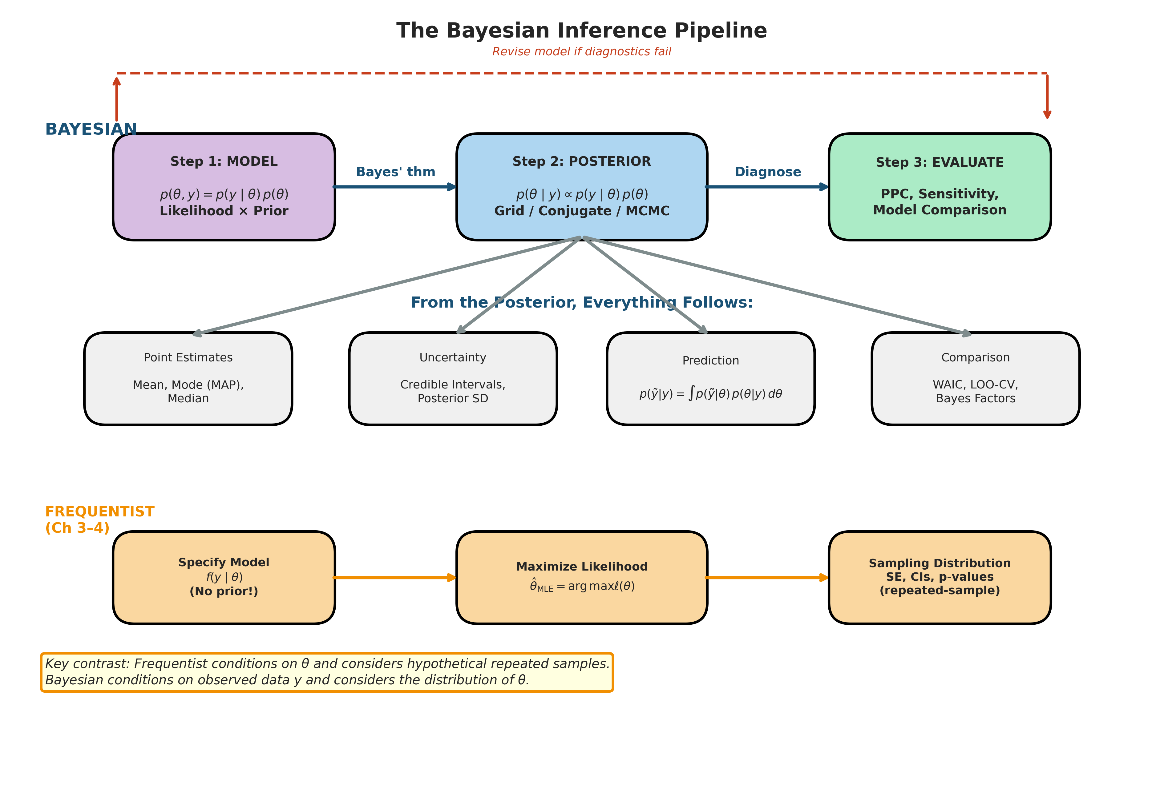
Fig. 172 Figure 5.1: The Bayesian Inference Pipeline. The top row shows the three-step Bayesian workflow: specify a joint model \(p(\theta, y) = p(y \mid \theta) \, p(\theta)\) (Step 1), compute the posterior \(p(\theta \mid y)\) via grid approximation, conjugate analysis, or MCMC (Step 2), and evaluate model fit through posterior predictive checks and sensitivity analysis (Step 3), with a feedback loop for model revision. From the posterior, four classes of inference follow directly: point estimates, uncertainty quantification, prediction, and model comparison. The bottom row shows the frequentist pipeline from Chapters 3–4 for contrast: it begins with a likelihood alone (no prior), maximizes to obtain the MLE, and quantifies uncertainty through the sampling distribution. The key distinction is that the frequentist conditions on \(\theta\) and considers hypothetical repeated samples, whereas the Bayesian conditions on the observed data \(y\) and considers the distribution of \(\theta\).
Bayes’ Theorem for Parameters
Section 1.1 introduced Bayes’ theorem as a mathematical identity relating conditional probabilities. Here we deepen that treatment, focusing on the specific form needed for parametric inference with continuous parameters.
The Posterior Distribution
Suppose we observe data \(y = (y_1, \ldots, y_n)\) from a model with parameter \(\theta \in \Theta \subseteq \mathbb{R}^d\). Bayes’ theorem yields the posterior density:
where the denominator is the marginal likelihood \(p(y)\). Each component of this equation plays a distinct role, and understanding these roles is essential for both computation and interpretation. We now define each component formally.
Definition: Prior Distribution
The prior distribution \(p(\theta)\) is a probability distribution over the parameter space \(\Theta\) that encodes the analyst’s state of knowledge about \(\theta\) before observing the data \(y\). The prior may reflect:
Genuine scientific knowledge (e.g., a treatment effect is expected to be positive)
Physical constraints (e.g., a probability must lie in \([0,1]\), a variance must be positive)
Deliberate agnosticism (e.g., a flat or weakly informative prior expressing minimal assumptions)
The prior is a probability distribution in its own right: it integrates to one (for proper priors), has a mean, variance, and quantiles. A prior is called improper if \(\int p(\theta) \, d\theta = \infty\); improper priors can still yield proper posteriors if the likelihood provides sufficient information, but they must be used with care. We develop strategies for choosing priors systematically in Section 5.2 Prior Specification and Conjugate Analysis.
The likelihood \(p(y \mid \theta)\) — also written \(L(\theta) = L(\theta; y)\) — is the probability (or probability density) of the observed data given the parameter value. This is the same likelihood function that we maximized to obtain the MLE in Chapter 3. For independent observations \(y_1, \ldots, y_n\) from \(f(y \mid \theta)\):
The likelihood is not a probability distribution over \(\theta\) — it does not integrate to one as \(\theta\) varies. It is a function of \(\theta\) that tells us how well each parameter value “explains” the observed data. Large likelihood values indicate parameter values that make the data probable; small values indicate parameter values under which the data would be surprising. This distinction matters: the prior is a distribution, the likelihood is a function, and the posterior is a distribution. Only the prior and posterior integrate to one (over \(\theta\)); the likelihood integrates to one over \(y\) (for each fixed \(\theta\)), not over \(\theta\).
Definition: Marginal Likelihood (Evidence)
The marginal likelihood (also called the evidence or prior predictive distribution) is the normalizing constant in Bayes’ theorem:
It is the probability of the observed data averaged over all parameter values, weighted by the prior. The marginal likelihood serves two distinct roles:
Normalization: It ensures \(\int p(\theta \mid y) \, d\theta = 1\), making the posterior a proper probability distribution.
Model comparison: Two competing models \(M_1\) and \(M_2\) can be compared via the Bayes factor \(B_{12} = p(y \mid M_1) / p(y \mid M_2)\), the ratio of their marginal likelihoods (developed in Section 5.7 Bayesian Model Comparison).
For most posterior inference — point estimates, credible intervals, prediction — the marginal likelihood is not needed, because the unnormalized posterior suffices. Computing \(p(y)\) requires evaluating an integral over the entire parameter space, which is the central computational challenge of the Bayesian framework.
Definition: Posterior Distribution
The posterior distribution \(p(\theta \mid y)\) is the conditional distribution of the parameter \(\theta\) given the observed data \(y\), obtained via Bayes’ theorem (126):
The posterior is the complete Bayesian answer: it represents the analyst’s updated state of knowledge about \(\theta\) after combining prior information with the evidence from the data. Every inferential quantity in Bayesian analysis is derived from it:
Point estimates (posterior mean, median, or mode)
Interval estimates (credible intervals, Section 5.3 Posterior Inference: Credible Intervals and Hypothesis Assessment)
Predictions (posterior predictive distribution)
Model evaluation (posterior predictive checks, Section 5.6 Probabilistic Programming with PyMC)
The three components — prior, likelihood, posterior — form a triad that captures the logic of learning from data. The prior says what we knew before; the likelihood says what the data tell us; the posterior says what we know now. Bayes’ theorem is the mechanism that combines the first two into the third.
The Proportional-To Form
Since \(p(y)\) is constant with respect to \(\theta\), we can write the most practically important form of Bayes’ theorem:
In words: the posterior is proportional to the likelihood times the prior. This unnormalized form is the workhorse of Bayesian computation. Grid approximation, MCMC, and optimization-based methods all work with the right-hand side, sidestepping the intractable integral in the denominator.
The “proportional to” symbol \(\propto\) means that the left and right sides are equal up to a multiplicative constant (in this case, \(1/p(y)\)). To recover the actual posterior density, we need only ensure it integrates to one — either analytically (conjugate models, Section 5.2 Prior Specification and Conjugate Analysis) or numerically (grid approximation below, or MCMC in Section 5.5 MCMC Algorithms: Metropolis-Hastings and Gibbs Sampling).
Working with the unnormalized posterior is not a shortcut or an approximation — it is a fundamental strategy that sidesteps the hardest computational problem in the entire framework. In a \(d\)-dimensional parameter space, computing the normalizing constant requires evaluating a \(d\)-dimensional integral, which is exactly the problem we spent Chapter 2 developing Monte Carlo methods to solve. The entire arc from grid approximation to MCMC can be understood as increasingly sophisticated strategies for working with \(p(\theta \mid y) \propto p(y \mid \theta) \, p(\theta)\) without ever computing \(p(y)\) directly.
It is worth pausing to appreciate how remarkable this is. In frequentist inference, we needed the exact sampling distribution of our estimator (or an asymptotic approximation to it) to construct confidence intervals and tests. In Bayesian inference, we only need the unnormalized posterior — a product of two functions we can evaluate pointwise. The normalizing constant is the price of turning a relative weighting into a proper probability distribution, but for many purposes (finding the posterior mode, computing posterior means via Monte Carlo, simulating from the posterior via MCMC) we never need to pay that price.
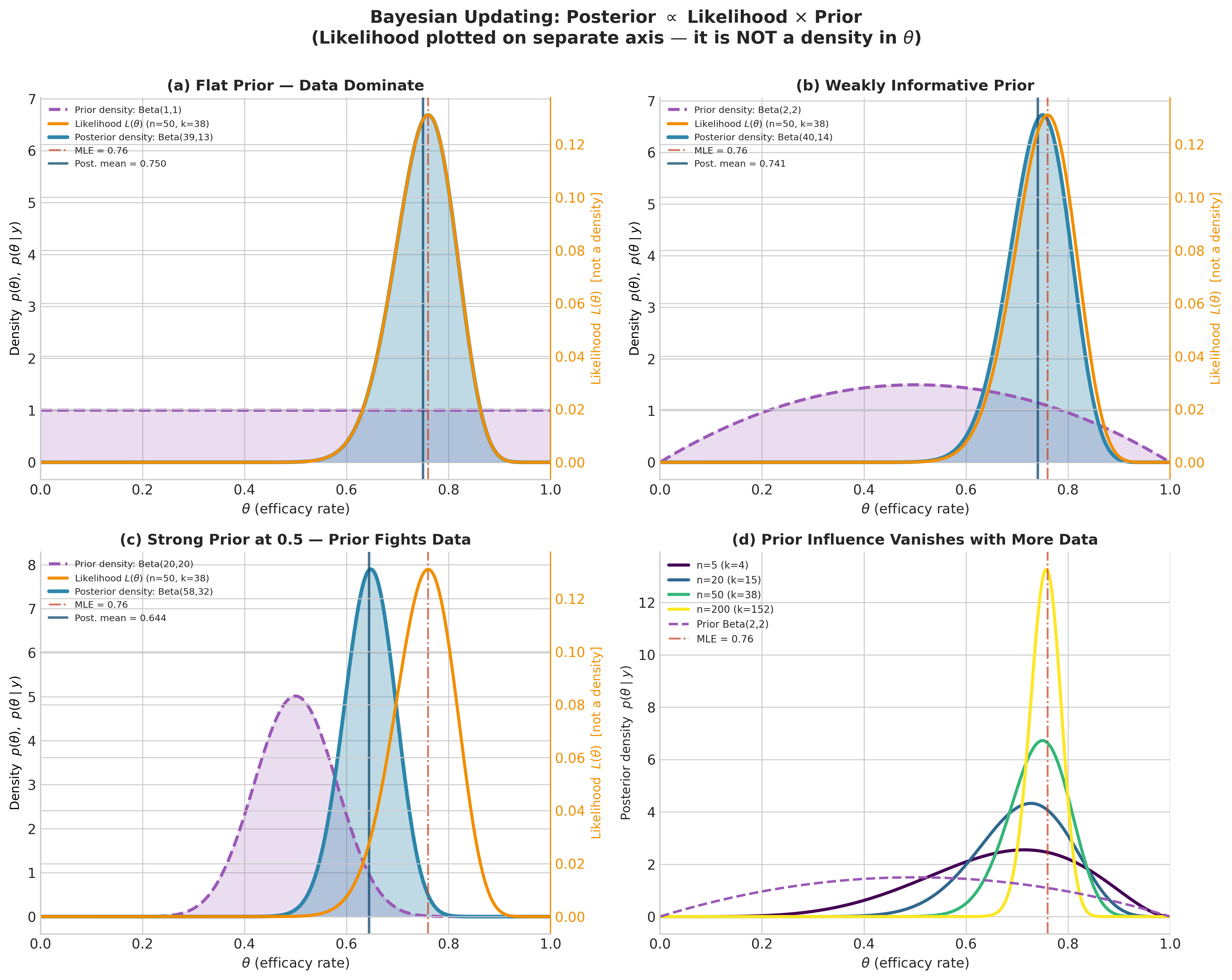
Fig. 173 Figure 5.2: Bayesian Updating: Posterior \(\propto\) Likelihood \(\times\) Prior. Panels (a–c) show the vaccine trial data (\(k = 38\) successes in \(n = 50\) trials) under three priors of increasing strength. The prior density and posterior density share the left axis (both integrate to one over \(\theta\)); the likelihood \(L(\theta)\) is plotted on the right axis to emphasize that it is a function of \(\theta\), not a probability density. Under a flat prior (a), the posterior nearly coincides with the likelihood. Under a strong Beta(20, 20) prior centered at 0.5 (c), the posterior is visibly pulled toward the prior, away from the MLE at 0.76 — this is shrinkage. Panel (d) demonstrates that the prior’s influence vanishes as sample size grows: posteriors at \(n = 5, 20, 50, 200\) (all with \(k/n = 0.76\)) concentrate around the MLE regardless of the Beta(2, 2) prior. Axes label \(\theta\) as efficacy rate as informal shorthand; this is technically the single-arm response rate (see the Terminology Note above).
Example 💡 Unnormalized Posterior in One Dimension
Given: A single observation \(y = 3\) from a Poisson(\(\lambda\)) distribution with a Gamma(2, 1) prior on \(\lambda\).
Find: The unnormalized posterior and verify it yields a recognizable distribution.
Mathematical approach:
The likelihood for a single Poisson observation is \(p(y \mid \lambda) = e^{-\lambda} \lambda^y / y!\) and the Gamma(2, 1) prior density is \(p(\lambda) = \lambda \, e^{-\lambda}\) for \(\lambda > 0\). Applying the proportional-to form:
We dropped the constant \(1/3!\) because it does not depend on \(\lambda\). The kernel of a density is the part of the expression that depends on the parameter — all multiplicative constants that do not involve \(\lambda\) can be dropped without changing the shape of the distribution. The remaining expression \(\lambda^4 \, e^{-2\lambda}\) is the kernel of a Gamma(5, 2) density — that is, a Gamma distribution with shape \(\alpha = 5\) and rate \(\beta = 2\). This is precisely the conjugate update rule from Section 3.1 Exponential Families: \(\text{Gamma}(\alpha + y, \, \beta + 1) = \text{Gamma}(2 + 3, \, 1 + 1)\).
The identification of the posterior by recognizing the kernel — the terms that depend on \(\lambda\) — is a skill that becomes second nature with practice. For exponential family models with conjugate priors, the posterior always belongs to the same family as the prior, and the hyperparameters update by simple addition rules. The general theory is in Section 5.2 Prior Specification and Conjugate Analysis.
Python verification:
import numpy as np
from scipy import stats

# Parameters
alpha_prior, beta_prior = 2, 1  # Gamma(2, 1) prior
y_obs = 3                        # Observed count

# Conjugate update: Gamma(alpha + y, beta + n)
alpha_post = alpha_prior + y_obs  # = 5
beta_post = beta_prior + 1        # = 2

posterior = stats.gamma(a=alpha_post, scale=1/beta_post)
print(f"Posterior: Gamma({alpha_post}, {beta_post})")
print(f"Posterior mean:  {posterior.mean():.4f}")
print(f"Posterior mode:  {(alpha_post - 1) / beta_post:.4f}")
print(f"Prior mean:      {alpha_prior / beta_prior:.4f}")
print(f"MLE (flat prior): {y_obs:.4f}")
Posterior: Gamma(5, 2)
Posterior mean:  2.5000
Posterior mode:  2.0000
Prior mean:      2.0000
MLE (flat prior): 3.0000
Result: The posterior mean (2.5) lies between the prior mean (2.0) and the MLE (3.0), illustrating how the posterior is a compromise between prior information and data evidence. The prior pulls the estimate downward from the MLE — a phenomenon called shrinkage: the posterior estimate is pulled, or shrunk, toward the prior mean relative to the MLE, with the degree of shrinkage determined by the ratio of prior strength to sample size. We will encounter this pattern repeatedly throughout this chapter. With only a single observation, the prior has substantial influence; as we accumulate more data, the posterior will concentrate around the MLE, a consequence of the Bernstein-von Mises theorem discussed in Section 3.3 Sampling Variability and Variance Estimation.
Discrete Parameter Spaces
When the parameter space is discrete (or finite), the integral in the marginal likelihood becomes a sum, and Bayes’ theorem can be applied directly without any approximation or advanced computation. Discrete examples are pedagogically invaluable because they make the entire mechanism transparent — every probability can be computed by hand, every step can be verified. The intuitions we build here transfer directly to the continuous case.
The Mechanics of Discrete Updating
For a discrete parameter \(\theta \in \{\theta_1, \ldots, \theta_K\}\), Bayes’ theorem (126) becomes:
The computation is entirely mechanical: multiply each prior probability by the corresponding likelihood, then normalize by dividing by the sum. The result is a new probability distribution over the same set of hypotheses, but now informed by the data.
This is the discrete version of the “multiply and normalize” recipe that defines all Bayesian inference. The simplicity of the discrete case belies its power: it handles arbitrary numbers of competing hypotheses, accommodates any pattern of prior beliefs, and extends effortlessly to sequential updating.
Sequential Bayesian Updating
One of the most elegant properties of Bayesian inference is sequential updating: today’s posterior becomes tomorrow’s prior. If we observe data in batches \(y_1, y_2, \ldots\), then after the first batch the posterior is \(p(\theta \mid y_1)\), and after the second batch:
This means Bayesian inference is inherently online — we can update our beliefs as new data arrive without reprocessing old data. For a sequence of \(n\) independent observations:
The order of observations does not matter (by commutativity of multiplication), but the sequential perspective is both computationally useful and conceptually illuminating. It makes concrete the idea that Bayesian learning is cumulative: each piece of evidence modifies our beliefs, and the posterior after all the evidence is exactly the same whether we process the evidence one observation at a time or all at once.
This property has profound practical implications. Because the factorization in (131) does not depend on the order of terms, in clinical trials we can continuously update our assessment of a drug’s efficacy as patients are enrolled, rather than waiting until the trial is complete. In online recommendation systems, we can update user preference models with each new click. In environmental monitoring, we can incorporate each new sensor reading into our estimate of pollution levels. The formal coherence of sequential Bayesian updating — the guarantee that the final answer does not depend on the order or grouping of observations — gives these applications a rigorous foundation that purely ad hoc approaches lack.
Example 💡 Disease Diagnosis with Sequential Tests
Given: A genetic screening problem. An individual’s genotype is one of three possible types: \(\theta \in \{A, B, C\}\), with population-level prior probabilities \(p(A) = 0.50\), \(p(B) = 0.25\), \(p(C) = 0.25\). Two diagnostic tests are performed sequentially, each with known error characteristics:
Test 1 result: positive. Likelihoods: \(p(+ \mid A) = 0.80\), \(p(+ \mid B) = 0.40\), \(p(+ \mid C) = 0.10\).
Test 2 result: negative. Likelihoods: \(p(- \mid A) = 0.30\), \(p(- \mid B) = 0.60\), \(p(- \mid C) = 0.90\).
Find: The posterior probability of each genotype after both tests, using sequential updating.
Mathematical approach (sequential updating):
After Test 1 (positive):
Compute unnormalized posteriors by multiplying each prior by the corresponding likelihood:
Normalizing constant: \(p(+) = 0.400 + 0.100 + 0.025 = 0.525\). Dividing each unnormalized value by 0.525:
The positive test strongly favored genotype A, increasing its probability from the prior value of 50% to 76%.
After Test 2 (negative), using the Test 1 posterior as the new prior:
Normalizing: sum = \(0.3857\). Dividing:
Python implementation:
import numpy as np

# Prior probabilities
prior = np.array([0.50, 0.25, 0.25])
genotypes = ['A', 'B', 'C']

# Test 1 likelihoods (positive result)
lik_test1 = np.array([0.80, 0.40, 0.10])

# Update after Test 1: multiply and normalize
unnorm_post1 = lik_test1 * prior
post1 = unnorm_post1 / unnorm_post1.sum()
print("After Test 1 (positive):")
for g, p in zip(genotypes, post1):
    print(f"  P({g} | +) = {p:.4f}")

# Test 2 likelihoods (negative result)
lik_test2 = np.array([0.30, 0.60, 0.90])

# Sequential update: use post1 as prior
unnorm_post2 = lik_test2 * post1
post2 = unnorm_post2 / unnorm_post2.sum()
print("\nAfter Test 2 (negative):")
for g, p in zip(genotypes, post2):
    print(f"  P({g} | +, -) = {p:.4f}")

# Verify: batch update gives same result
unnorm_batch = lik_test1 * lik_test2 * prior
post_batch = unnorm_batch / unnorm_batch.sum()
print("\nBatch update (both tests at once):")
for g, p in zip(genotypes, post_batch):
    print(f"  P({g} | +, -) = {p:.4f}")
After Test 1 (positive):
  P(A | +) = 0.7619
  P(B | +) = 0.1905
  P(C | +) = 0.0476

After Test 2 (negative):
  P(A | +, -) = 0.5926
  P(B | +, -) = 0.2963
  P(C | +, -) = 0.1111

Batch update (both tests at once):
  P(A | +, -) = 0.5926
  P(B | +, -) = 0.2963
  P(C | +, -) = 0.1111
Result: Sequential and batch updates yield identical posteriors, confirming the coherence of Bayesian updating. The positive first test strongly favored genotype A (from 50% to 76%), but the negative second test moderated that conclusion (back to 59%) because genotype A has a relatively low probability of producing a negative result (only 30%), whereas genotypes B and C produce negative results more readily (60% and 90%). The two tests “pull” in opposite directions for genotype A, and the posterior reflects this tension. Notice that genotype C, despite having the highest probability of a negative result, retains only 11% posterior probability because it was so strongly disfavored by the first test — a mere 2.5% of the prior-weighted likelihood.
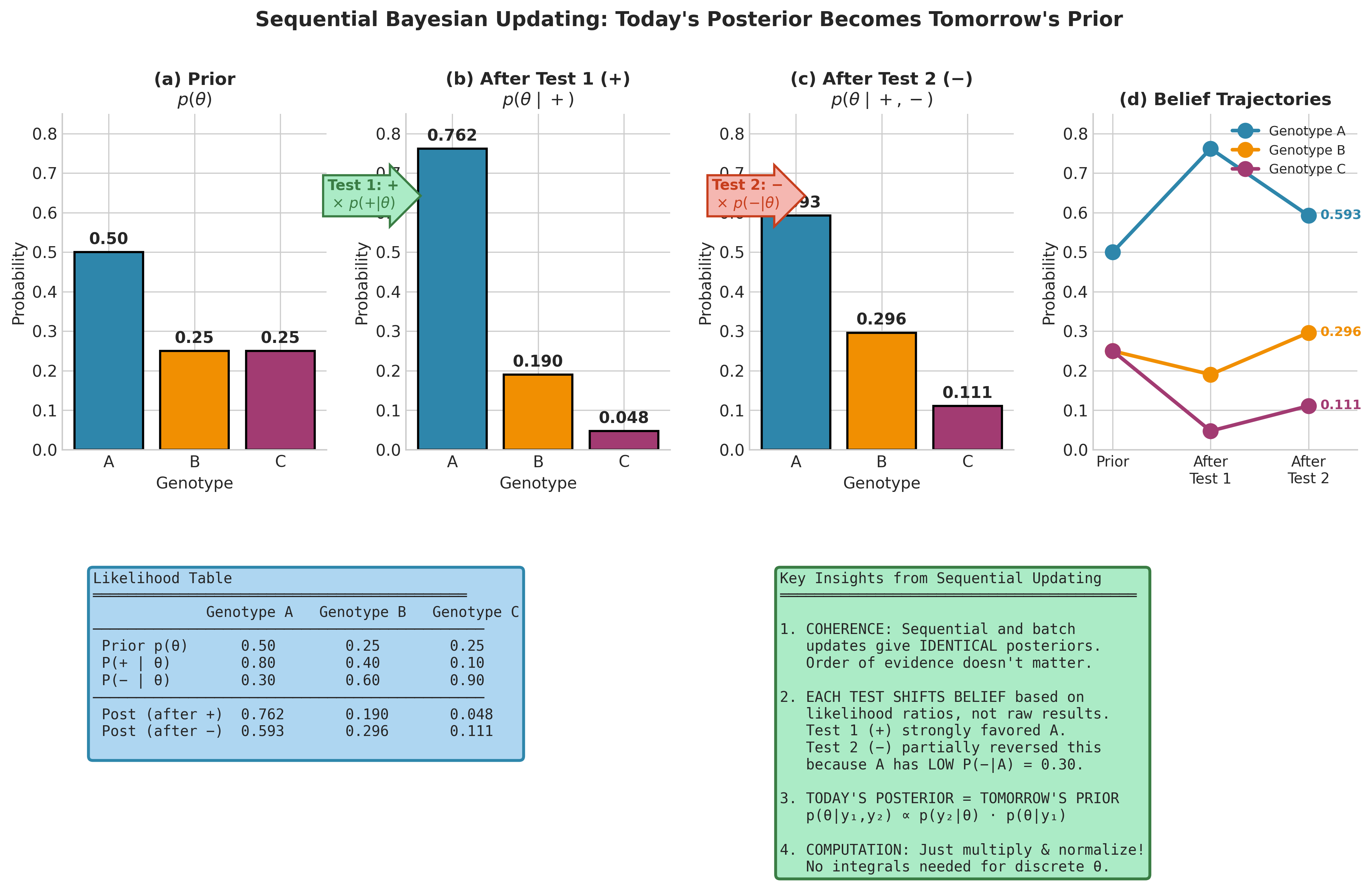
Fig. 174 Figure 5.3: Sequential Bayesian Updating for Genetic Diagnosis. Panels (a–c) show the probability distribution over three genotypes evolving as evidence accumulates: the prior (a) is updated by a positive diagnostic test (b), then by a negative test (c). Panel (d) tracks the belief trajectories — genotype A rises sharply after the positive test but retreats after the negative test, while genotypes B and C move in opposite directions. The likelihood table (bottom left) records the data driving each update. The key insight: today’s posterior becomes tomorrow’s prior, and sequential and batch processing yield identical results.
Continuous Parameters: Grid Approximation
For continuous parameters, the marginal likelihood integral (127) typically has no closed-form solution. Before developing the elegant analytical machinery of conjugate analysis (Section 5.2 Prior Specification and Conjugate Analysis) and the powerful general-purpose MCMC algorithms (Section 5.5 MCMC Algorithms: Metropolis-Hastings and Gibbs Sampling), we introduce a conceptually transparent computational strategy: grid approximation.
The idea is simple and directly extends how we just handled the discrete case. Starting from the proportional-to form (129), we discretize the continuous parameter space into a fine grid of points, evaluate the unnormalized posterior at each point, and normalize by the sum. As the grid becomes finer, the approximation converges to the true posterior. Grid approximation is the Bayesian analog of the rectangle rule from numerical integration (see Appendix C for quadrature error rates and when finer methods are needed) — crude but reliable, and invaluable for building intuition.
Mathematical Framework
For a one-dimensional parameter \(\theta \in [\theta_{\min}, \theta_{\max}]\), choose \(n_g\) equally spaced grid points \(\theta_1, \ldots, \theta_{n_g}\) with spacing \(\Delta\theta = (\theta_{\max} - \theta_{\min}) / (n_g-1)\). The grid approximation to the posterior is:
where the summation in the denominator approximates the integral \(\int p(y \mid \theta) p(\theta) \, d\theta\) by a Riemann sum. For practical computation, we need only the relative probabilities:
This is exactly the “multiply and normalize” recipe from the discrete case, applied to a discretized version of the continuous parameter space. The grid approximation converts an intractable integral into a tractable sum.
Extension to two dimensions. For parameters \((\theta_1, \theta_2)\), we construct a two-dimensional grid with \(n_{g,1} \times n_{g,2}\) points. The unnormalized posterior is evaluated at each grid cell:
and normalized by \(\sum_{j,k} w_{jk}\). The marginal posterior for \(\theta_1\) is obtained by summing over \(\theta_2\):
This summation-based marginalization is the discrete analog of the integral \(p(\theta_1 \mid y) = \int p(\theta_1, \theta_2 \mid y) \, d\theta_2\), and it generalizes straightforwardly to marginalization over any subset of parameters.
Computational Perspective
Grid approximation is simple to implement and easy to understand, but it has a fundamental scalability limitation that must be understood clearly.
Algorithm: Grid Approximation (1D)
Input: Prior function p(θ), likelihood function p(y|θ),
       grid bounds [θ_min, θ_max], number of grid points n_g
Output: Approximate posterior probabilities on grid

1. Create grid: θ_1, ..., θ_{n_g} equally spaced in [θ_min, θ_max]
2. For j = 1, ..., n_g:
   a. Compute log unnormalized posterior:
      log w_j = log p(y|θ_j) + log p(θ_j)
3. Normalize using log-sum-exp:
   a. m = max(log w_1, ..., log w_{n_g})
   b. log Z = m + log Σ_k exp(log w_k - m)
   c. log p̂(θ_j|y) = log w_j - log Z
4. Return grid values θ_1,...,θ_{n_g} and posterior weights exp(log p̂)
Computational complexity: \(O(n_g^{\,d})\) where \(d\) is the dimension of the parameter space and \(n_g\) is the number of grid points per dimension. For \(d = 1\) with \(n_g = 1000\), this is trivial — a fraction of a second on any modern computer. For \(d = 2\) with \(n_g = 100\) per dimension, we evaluate 10,000 points — still fast. But the exponential growth is unforgiving: for \(d = 5\) with \(n_g = 50\), we need \(50^5 \approx 3 \times 10^8\) evaluations (slow but feasible), and for \(d = 10\) with \(n_g = 20\), we need \(20^{10} \approx 10^{13}\) evaluations (completely infeasible on any current hardware).
This is the curse of dimensionality, and it is the fundamental reason that MCMC methods (Section 5.4 Markov Chains: The Mathematical Foundation of MCMC, Section 5.5 MCMC Algorithms: Metropolis-Hastings and Gibbs Sampling) were developed. Grid approximation exhaustively enumerates the parameter space; MCMC explores it adaptively, concentrating computation where the posterior has appreciable mass.
Numerical stability. When the likelihood involves many observations, \(p(y \mid \theta)\) can be astronomically small (or large) for some \(\theta\) values, causing floating-point underflow or overflow (see Appendix C for IEEE 754 representation and log-space arithmetic). The standard remedy is to work on the log scale:
and then use the log-sum-exp trick (introduced in Section 2.6 Variance Reduction Methods) for normalization:
where \(\text{logsumexp}(a_1, \ldots, a_{n_g}) = a_{\max} + \log \sum_{k=1}^{n_g} \exp(a_k - a_{\max})\). The subtraction of \(a_{\max}\) prevents overflow; the subsequent addition restores the correct scale. This technique is not optional — it is a requirement for numerically correct results with any dataset of realistic size.
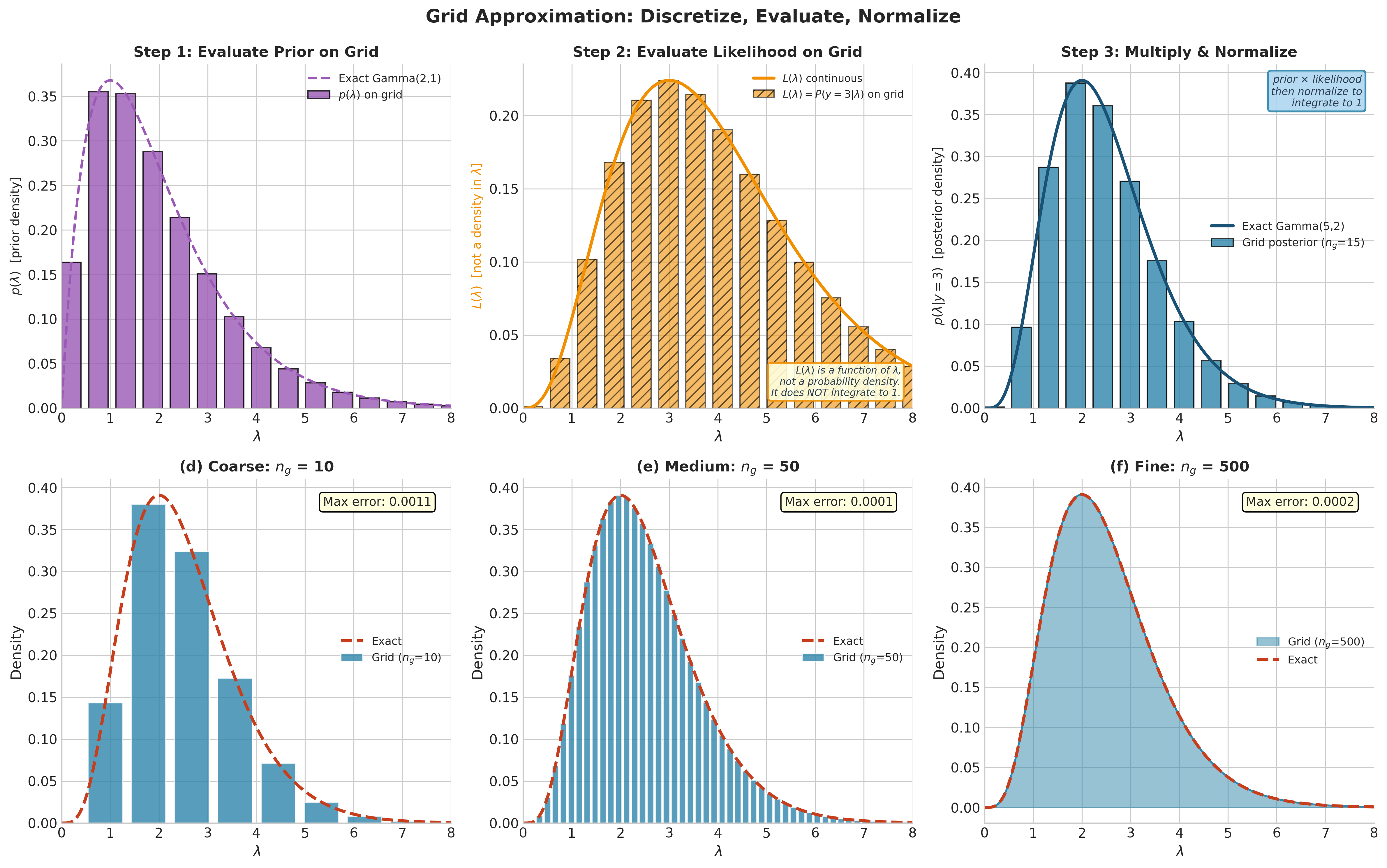
Fig. 175 Figure 5.4: Grid Approximation: Discretize, Evaluate, Normalize. Top row demonstrates the three-step algorithm for a Poisson observation \(y = 3\) with Gamma(2, 1) prior. Step 1 evaluates the prior density on a coarse 15-point grid. Step 2 evaluates the likelihood \(L(\lambda) = P(y{=}3 \mid \lambda)\) — note the hatched bars and separate axis label emphasizing that \(L(\lambda)\) is a function of \(\lambda\), not a probability density. Step 3 multiplies prior by likelihood and normalizes to obtain the posterior, which closely matches the exact Gamma(5, 2). Bottom row shows convergence as the grid refines: at \(n_g = 10\) the approximation is rough, at \(n_g = 50\) it closely tracks the exact posterior, and at \(n_g = 500\) the two are visually indistinguishable.
Python Implementation
The following implementation encapsulates the grid approximation algorithm with log-scale computation throughout. Both functions accept arbitrary log-prior and log-likelihood callables, making them applicable to any model.
import numpy as np
from scipy import stats
from scipy.special import logsumexp

def grid_posterior_1d(log_prior_func, log_likelihood_func, grid):
    """
    Compute posterior distribution on a 1D grid via grid approximation.

    Uses log-scale arithmetic throughout for numerical stability.
    The log-sum-exp trick prevents underflow/overflow when the
    likelihood spans many orders of magnitude.

    Parameters
    ----------
    log_prior_func : callable
        Function mapping theta -> log p(theta).
    log_likelihood_func : callable
        Function mapping theta -> log p(y | theta).
    grid : np.ndarray
        1D array of parameter values to evaluate.

    Returns
    -------
    dict
        Keys: 'grid', 'log_posterior', 'posterior' (normalized weights),
        'density' (density-scale values), 'mean', 'mode', 'std'.
    """
    # Evaluate log unnormalized posterior on grid
    log_prior = np.array([log_prior_func(t) for t in grid])
    log_lik = np.array([log_likelihood_func(t) for t in grid])
    log_unnorm = log_prior + log_lik

    # Normalize using log-sum-exp for numerical stability
    log_posterior = log_unnorm - logsumexp(log_unnorm)
    posterior = np.exp(log_posterior)

    # Posterior summaries
    dx = grid[1] - grid[0] if len(grid) > 1 else 1.0
    posterior_norm = posterior / (posterior.sum() * dx)  # density scale
    mean = np.sum(grid * posterior) / posterior.sum()
    mode = grid[np.argmax(posterior)]
    var = np.sum((grid - mean)**2 * posterior) / posterior.sum()

    return {
        'grid': grid,
        'log_posterior': log_posterior,
        'posterior': posterior / posterior.sum(),
        'density': posterior_norm,
        'mean': mean,
        'mode': mode,
        'std': np.sqrt(var)
    }


def grid_posterior_2d(log_prior_func, log_likelihood_func, grid_x, grid_y):
    """
    Compute posterior distribution on a 2D grid (vectorized).

    Constructs a meshgrid from grid_x and grid_y and evaluates the
    unnormalized log-posterior in a single vectorized pass. Both
    callable arguments must accept 2D NumPy arrays (the meshgrid
    matrices) and return arrays of the same shape.

    Parameters
    ----------
    log_prior_func : callable
        Function mapping (Theta1, Theta2) -> log p(Theta1, Theta2),
        where Theta1 and Theta2 are 2D arrays from np.meshgrid.
    log_likelihood_func : callable
        Function mapping (Theta1, Theta2) -> log p(y | Theta1, Theta2),
        where Theta1 and Theta2 are 2D arrays from np.meshgrid.
    grid_x, grid_y : np.ndarray
        1D arrays of parameter values for each dimension.

    Returns
    -------
    dict
        Keys: 'grid_x', 'grid_y', 'joint_posterior' (n_x × n_y array),
        'marginal_x', 'marginal_y', 'mode' (tuple).
    """
    # Build 2D meshgrid — 'ij' indexing so axis 0 = grid_x
    TX, TY = np.meshgrid(grid_x, grid_y, indexing='ij')

    # Vectorized evaluation: no Python loops
    log_unnorm = log_prior_func(TX, TY) + log_likelihood_func(TX, TY)

    # Normalize via log-sum-exp
    log_posterior = log_unnorm - logsumexp(log_unnorm.ravel())
    joint = np.exp(log_posterior)
    joint /= joint.sum()

    # Marginals by summation
    marginal_x = joint.sum(axis=1)
    marginal_x /= marginal_x.sum()
    marginal_y = joint.sum(axis=0)
    marginal_y /= marginal_y.sum()

    # Joint mode
    idx = np.unravel_index(np.argmax(joint), joint.shape)
    mode = (grid_x[idx[0]], grid_y[idx[1]])

    return {
        'grid_x': grid_x, 'grid_y': grid_y,
        'joint_posterior': joint,
        'marginal_x': marginal_x, 'marginal_y': marginal_y,
        'mode': mode
    }
We now put grid approximation to work on a real Beta-Binomial problem. Rather than the stylized vaccine trial that motivated this section, we use a dataset where the constant-\(\theta\), exchangeable-trials assumption is genuinely defensible — free-throw shooting — and check the grid answer against the exact conjugate posterior.
Example 💡 Beta-Binomial: Grid Approximation vs. Conjugate Analysis
Given: Over the 2023-24 NBA season, Stephen Curry made \(k = 299\) of \(n = 324\) free throws. We place a flat Beta(1, 1) prior on his true make rate \(\theta\) and let the data speak. (Free throws — not three-pointers — because the Beta-Binomial assumes a single constant \(\theta\) across exchangeable iid trials: same distance, no defender, identical routine.)
Find: The posterior distribution of \(\theta\) using (a) grid approximation and (b) the analytical conjugate formula. Compare the two approaches quantitatively.
Mathematical approach:
The flat Beta(1, 1) prior has density \(p(\theta) \propto 1\) on \([0,1]\). The Binomial likelihood is \(p(y=299 \mid \theta) \propto \theta^{299}(1-\theta)^{25}\). The unnormalized posterior is therefore:
This is the kernel of a Beta(300, 26) density. By the conjugate update rule from Section 3.1 Exponential Families:
The posterior mean and mode are:
With a flat prior the posterior mode equals the MLE \(k/n = 299/324 = 0.9228\).
Python implementation:
import numpy as np
from scipy import stats
from scipy.special import logsumexp

# Data: Curry's 2023-24 free throws (real; vendored in BDA/, see scripts/ch5/01)
n, k = 324, 299

# Flat prior: Beta(1, 1)
alpha_prior, beta_prior = 1, 1

# --- Method 1: Grid approximation ---
n_g = 1000
theta_grid = np.linspace(0.001, 0.999, n_g)

# Log prior and log likelihood on grid
log_prior = stats.beta.logpdf(theta_grid, alpha_prior, beta_prior)
log_lik = stats.binom.logpmf(k, n, theta_grid)
log_unnorm = log_prior + log_lik

# Normalize via log-sum-exp
log_post_grid = log_unnorm - logsumexp(log_unnorm)
post_grid = np.exp(log_post_grid)
post_grid /= post_grid.sum()

# Grid-based summaries
grid_mean = np.sum(theta_grid * post_grid)
grid_mode = theta_grid[np.argmax(post_grid)]
grid_std = np.sqrt(np.sum((theta_grid - grid_mean)**2 * post_grid))
grid_p_elite = post_grid[theta_grid > 0.90].sum()

# --- Method 2: Analytical conjugate ---
alpha_post = alpha_prior + k      # = 300
beta_post = beta_prior + (n - k)  # = 26
exact_posterior = stats.beta(alpha_post, beta_post)

print("Grid Approximation (n_g=1000):")
print(f"  Mean:  {grid_mean:.4f}")
print(f"  Mode:  {grid_mode:.4f}")
print(f"  Std:   {grid_std:.4f}")
print(f"  P(theta > 0.90): {grid_p_elite:.4f}")
print(f"\nExact Conjugate Beta({alpha_post}, {beta_post}):")
print(f"  Mean:  {exact_posterior.mean():.4f}")
print(f"  Mode:  {(alpha_post - 1) / (alpha_post + beta_post - 2):.4f}")
print(f"  Std:   {exact_posterior.std():.4f}")
print(f"  P(theta > 0.90): {exact_posterior.sf(0.90):.4f}")
print(f"\nMLE (no prior information): {k/n:.4f}")
Grid Approximation (n_g=1000):
  Mean:  0.9202
  Mode:  0.9228
  Std:   0.0150
  P(theta > 0.90): 0.9024

Exact Conjugate Beta(300, 26):
  Mean:  0.9202
  Mode:  0.9228
  Std:   0.0150
  P(theta > 0.90): 0.9056

MLE (no prior information): 0.9228
Result: The grid approximation with 1,000 points matches the exact conjugate posterior to four decimals on the mean and three on \(P(\theta > 0.90)\) (the small gap reflects grid resolution near the boundary). With a flat prior and \(n = 324\) trials, the prior contributes only 2 pseudo-observations, so the data completely dominate: the posterior mean (0.9202) sits essentially on the MLE (0.9228) — no appreciable shrinkage. The inference that matters here is the exceedance probability: \(P(\theta > 0.90 \mid y) \approx 0.91\), so on this season’s evidence Curry is, with high posterior probability, a truly elite (90%+) free-throw shooter. The posterior standard deviation (0.015) tracks the frequentist standard error (\(\sqrt{\hat{\theta}(1-\hat{\theta})/n} \approx 0.015\)), reflecting the Bernstein-von Mises convergence discussed in Section 3.3 Sampling Variability and Variance Estimation. The full runnable version is in scripts/ch5/01_beta_binomial_grid.py.
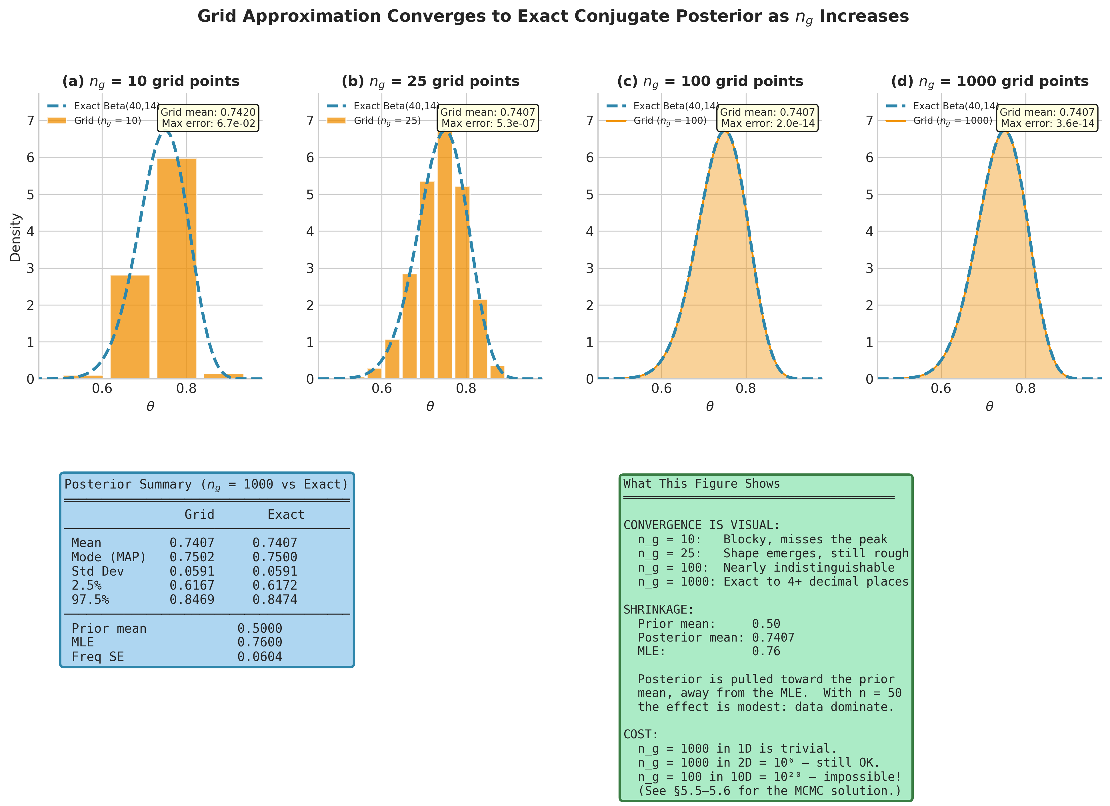
Fig. 176 Figure 5.5: Grid Approximation Converges to the Exact Conjugate Posterior. Top row: the grid posterior for Curry’s 2023-24 free throws (299 of 324) at four resolutions (\(n_g = 10, 25, 100, 1000\)) overlaid on the exact Beta(300, 26) posterior (dashed). At \(n_g = 10\) the approximation is visibly blocky and misses the sharp peak near 0.92; by \(n_g = 100\) it is nearly indistinguishable from the exact solution. The summary table (bottom left) confirms agreement to four decimal places at \(n_g = 1000\). Because the prior is flat, the posterior mean (0.9202) sits on the MLE (0.9228) — the \(n = 324\) observations completely dominate the prior’s 2 pseudo-observations, so there is no appreciable shrinkage.
The Curse of Dimensionality
The power of grid approximation fades rapidly as dimensionality increases. This is not a theoretical curiosity — it is the central computational barrier of Bayesian inference, and understanding it concretely motivates the MCMC machinery that occupies Sections 5.4–5.6.
Example 💡 Normal Mean and Variance: The 2D Case
Given: Michelson’s 1879 speed-of-light measurements — \(n = 100\) runs, recorded as km/s \(-\) 299,000 (the R morley dataset). Both the mean \(\mu\) and the standard deviation \(\sigma\) are unknown. We use vague priors: \(p(\mu) \propto 1\) (flat on the real line) and \(p(\sigma) \propto 1/\sigma\) for \(\sigma > 0\) (the Jeffreys prior for a scale parameter, motivated by invariance under rescaling — see Section 5.2 Prior Specification and Conjugate Analysis).
Find: The joint posterior \(p(\mu, \sigma \mid y)\) by grid approximation, then extract marginal posteriors for each parameter.
Mathematical approach:
The log-likelihood for \(n\) iid Normal observations is:
The log of the Jeffreys prior is \(\log p(\sigma) = -\log \sigma\) (plus a constant). For the flat prior on \(\mu\), the log-prior is constant. The unnormalized log-posterior is therefore:
We evaluate this on a 2D grid and marginalize by summing over each parameter.
Python implementation:
import numpy as np
import pandas as pd
from scipy.special import logsumexp

# Michelson's 1879 speed-of-light data (R datasets 'morley'),
# reported as km/s - 299000; n = 100 runs.
morley = pd.read_csv(
    "https://vincentarelbundock.github.io/Rdatasets/csv/datasets/morley.csv")
y = morley["Speed"].to_numpy()        # 100 values, mean 852.4, SD 79.0

n = len(y)
ybar = y.mean()
s = y.std(ddof=0)                      # MLE scale

print(f"Data: n={n}, ybar={ybar:.1f}, s={s:.1f}  (km/s - 299000)")

# 2D grid (fixed bounds spanning the plausible region)
ng_mu, ng_sigma = 200, 200
mu_grid    = np.linspace(820, 885, ng_mu)
sigma_grid = np.linspace(60, 105, ng_sigma)

# Vectorized log-posterior via broadcasting
# Key insight: ss = Σ(y_i - mu)^2 depends only on mu, not sigma.
# Compute ss as a column vector, then broadcast against sigma.
SIGMA = sigma_grid[np.newaxis, :]  # shape (1, ng_sigma)

# Sum of squared deviations: shape (ng_mu, 1)
ss = np.sum((y - mu_grid[:, np.newaxis])**2, axis=1, keepdims=True)

# Log-posterior on (ng_mu, ng_sigma) grid via broadcasting
log_lik = -n * np.log(SIGMA) - 0.5 * ss / SIGMA**2
log_prior = -np.log(SIGMA)  # Jeffreys prior for scale
log_unnorm = log_lik + log_prior

# Normalize
log_post = log_unnorm - logsumexp(log_unnorm.ravel())
joint = np.exp(log_post)
joint /= joint.sum()

# Marginal for mu (sum over sigma)
marginal_mu = joint.sum(axis=1)
marginal_mu /= marginal_mu.sum()
post_mu_mean = np.sum(mu_grid * marginal_mu)
post_mu_std = np.sqrt(np.sum((mu_grid - post_mu_mean)**2
                              * marginal_mu))

# Marginal for sigma (sum over mu)
marginal_sigma = joint.sum(axis=0)
marginal_sigma /= marginal_sigma.sum()
post_sigma_mean = np.sum(sigma_grid * marginal_sigma)

# Joint mode
idx = np.unravel_index(np.argmax(joint), joint.shape)

print(f"\nJoint posterior mode: mu={mu_grid[idx[0]]:.1f}, "
      f"sigma={sigma_grid[idx[1]]:.1f}")
print(f"Marginal posterior mean of mu: {post_mu_mean:.1f} "
      f"(SD: {post_mu_std:.2f})")
print(f"Marginal posterior mean of sigma: {post_sigma_mean:.1f}")
print(f"\nGrid evaluations: {ng_mu} x {ng_sigma} = "
      f"{ng_mu * ng_sigma:,}")
print(f"If d=10 with n_g=20/dim: {20**10:,.0f} evaluations "
      f"(infeasible!)")
Data: n=100, ybar=852.4, s=79.0  (km/s - 299000)

Joint posterior mode: mu=852.3, sigma=78.3
Marginal posterior mean of mu: 852.4 (SD: 7.98)
Marginal posterior mean of sigma: 79.6

Grid evaluations: 200 x 200 = 40,000
If d=10 with n_g=20/dim: 10,240,000,000,000 evaluations (infeasible!)
Result: The 2D grid with 40,000 evaluations runs in well under a second and produces accurate posteriors for this two-parameter problem. The marginal posterior of \(\mu\) is centered at 852.4 km/s (above 299,000) with a standard deviation of 7.98; the marginal posterior mean of \(\sigma\) (79.6) sits slightly above the joint-mode scale (78.3) because the posterior for a scale parameter is right-skewed. There is a deeper lesson hiding in plain sight: the air-corrected “true” speed of light is 734.5 on this scale (Stigler 1977), which lies roughly 15 posterior standard errors below the \(\mu\) marginal — far outside any credible interval. Michelson’s apparatus was precise but inaccurate: a genuine systematic bias that the data alone cannot reveal (the §5.2 case study returns to this). The grid faithfully recovers the scatter, but no amount of grid resolution can surface a bias that is not in the data.
That bias is one lesson; the curse of dimensionality is the other, and the final printed line makes it vivid: a model with 10 parameters — quite modest for real applications — would require over 10 trillion grid evaluations. Even at one microsecond per evaluation, that is roughly four months of computation. Hierarchical models, regression with many predictors, and mixture models routinely involve dozens or hundreds of parameters. Grid approximation simply cannot scale.
The gap between “works beautifully for two parameters” and “completely infeasible for ten” is the chasm that MCMC bridges. Where grid approximation evaluates the posterior exhaustively — at every point in a pre-specified grid — MCMC constructs a Markov chain whose stationary distribution is the posterior, generating samples from regions of high posterior probability without wasting computation on regions where the posterior is negligible. We develop this machinery starting in Section 5.4 Markov Chains: The Mathematical Foundation of MCMC.
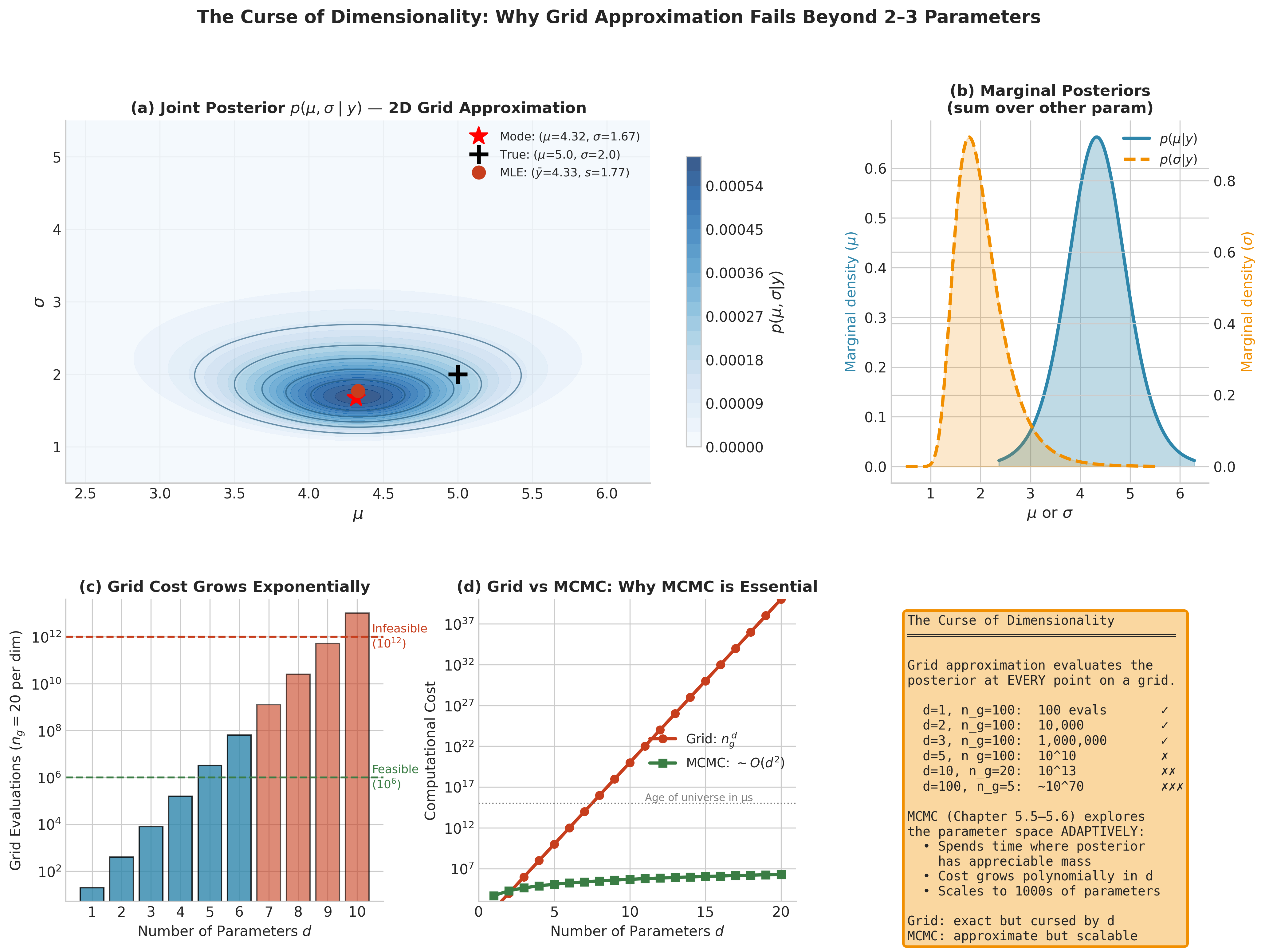
Fig. 177 Figure 5.6: The Curse of Dimensionality. Panel (a) shows the joint posterior \(p(\mu, \sigma \mid y)\) for Michelson’s speed-of-light data on a 200 × 200 grid — 40,000 evaluations that run in milliseconds — with the air-corrected truth 734.5 marked far to the left of the posterior mass (precise but inaccurate). Panel (b) displays the corresponding marginal posteriors obtained by summing over the other parameter. Panel (c) reveals the exponential cost: with \(n_g = 20\) grid points per dimension, the number of evaluations grows as \(n_g^{\,d}\), crossing the infeasibility threshold by \(d = 7\). Panel (d) contrasts this with MCMC, whose cost grows polynomially in \(d\), making it practical for models with hundreds or thousands of parameters.
The Posterior as Complete Inference
The posterior distribution \(p(\theta \mid y)\) is the complete Bayesian answer. Every inferential quantity is derived from it through straightforward probability calculations. This stands in contrast to the frequentist framework, where different inferential goals — point estimation, interval estimation, hypothesis testing, prediction — require separate theories and separate computational techniques. In the Bayesian framework, there is only the posterior; everything else is a summary or consequence of it.
Point Estimates
Three natural point estimates emerge from the posterior, each optimal under a different loss function. A loss function \(L(\theta, a)\) measures the cost of reporting the value \(a\) when the true parameter is \(\theta\). The Bayesian framework selects the estimate \(a\) that minimises the expected loss under the posterior — \(\mathbb{E}[L(\theta, a) \mid y]\). Different choices of loss function lead to different optimal estimates, formalising the intuition that the right summary depends on what errors are most costly in a given application.
Definition: Posterior Mean (Bayes Estimator)
The posterior mean is the expected value of the parameter under the posterior distribution:
The posterior mean minimizes the posterior expected squared error loss:
This makes it the Bayesian analog of choosing an estimator that minimizes mean squared error — the same criterion that motivates least-squares estimation in the frequentist framework.
Definition: Maximum A Posteriori (MAP) Estimate
The MAP estimate is the posterior mode — the parameter value with the highest posterior density:
The second equality follows because the marginal likelihood \(p(y)\) does not depend on \(\theta\). On the log scale:
This formulation reveals MAP estimation as penalized maximum likelihood: the log-prior acts as a penalty term that biases the estimate away from the MLE toward the prior mode.
The MAP estimate (134) provides the critical bridge between frequentist and Bayesian inference. Under a flat (constant) prior \(p(\theta) \propto 1\), the MAP estimate equals the MLE:
This connection — MLE as a special case of MAP estimation under a flat prior — provides a precise bridge between the frequentist methods of Chapter 3 and the Bayesian framework developed here. Under an informative prior, the MAP estimate is shifted away from the MLE toward the prior mode, implementing a form of regularization. Indeed, ridge regression corresponds to MAP estimation under a Normal(0, \(\tau^2\)) prior on regression coefficients (the \(L_2\) penalty \(\lambda \|\beta\|_2^2\) is exactly \(-\log p(\beta)\) up to an additive constant), and LASSO corresponds to a Laplace (double-exponential) prior (the \(L_1\) penalty \(\lambda \|\beta\|_1\) is \(-\log p(\beta)\)) — connections we noted in Section 3.4 Linear Models.
Posterior median: \(\tilde{\theta}_{\text{Bayes}}\) such that \(P(\theta \leq \tilde{\theta}_{\text{Bayes}} \mid y) = 0.5\). The posterior median minimizes the posterior expected absolute error loss \(\mathbb{E}[|\theta - a| \mid y]\). It is more robust to skewed posteriors than the mean and more interpretable than the mode when the posterior is highly asymmetric.
For symmetric posteriors (which arise from conjugate analysis with symmetric priors and sufficient data), all three estimates coincide. For skewed posteriors — common with small samples or bounded parameters — they diverge, and the choice depends on the loss function appropriate to the application. In practice, the posterior mean (133) is used most often, followed by the median for skewed posteriors. The MAP is conceptually useful (especially for its connection to the MLE and regularization) but less commonly reported as a stand-alone summary because it ignores the shape of the posterior — the mode of a heavily skewed distribution can be misleading about where most of the posterior mass lies.
The Posterior Predictive Distribution
A distinctive strength of Bayesian inference is prediction. Given the posterior, the posterior predictive distribution for a new observation \(\tilde{y}\) propagates all uncertainty — both about the parameter and about the data-generating process — into a single coherent prediction.
Definition: Posterior Predictive Distribution
The posterior predictive distribution for a future observation \(\tilde{y}\), given observed data \(y\), is:
This integral averages the sampling distribution \(p(\tilde{y} \mid \theta)\) over posterior uncertainty in \(\theta\). The result accounts for two sources of uncertainty:
Aleatoric uncertainty: the inherent randomness in data generation, captured by \(p(\tilde{y} \mid \theta)\)
Epistemic uncertainty: our uncertainty about the parameter, captured by \(p(\theta \mid y)\)
The posterior predictive is a genuine probability distribution over future data — it integrates to one over \(\tilde{y}\). Contrast this with the frequentist plug-in prediction \(p(\tilde{y} \mid \hat{\theta})\), which conditions on a single point estimate and ignores estimation uncertainty. The plug-in prediction is always narrower than the posterior predictive — it is overconfident because it treats the estimated parameter as if it were known exactly.
For the Beta-Binomial model, the posterior predictive for a new observation \(\tilde{y} \in \{0, 1\}\) takes a particularly clean form:
The posterior mean is the predictive probability of success. For more complex models, the predictive integral (135) may not have a closed form, but it can always be approximated by Monte Carlo sampling:
where \(\theta^{(1)}, \ldots, \theta^{(S)}\) are draws from the posterior. This connects directly to the Monte Carlo integration methods of Section 2.1 Monte Carlo Fundamentals, with the posterior replacing the distribution being integrated over. Drawing samples from the posterior — via conjugate formulas, grid-based sampling, or MCMC — and then simulating new data from each sample is one of the most practically useful techniques in Bayesian data analysis. We return to posterior prediction repeatedly throughout this chapter, and it plays a central role in model checking (Section 5.6 Probabilistic Programming with PyMC).
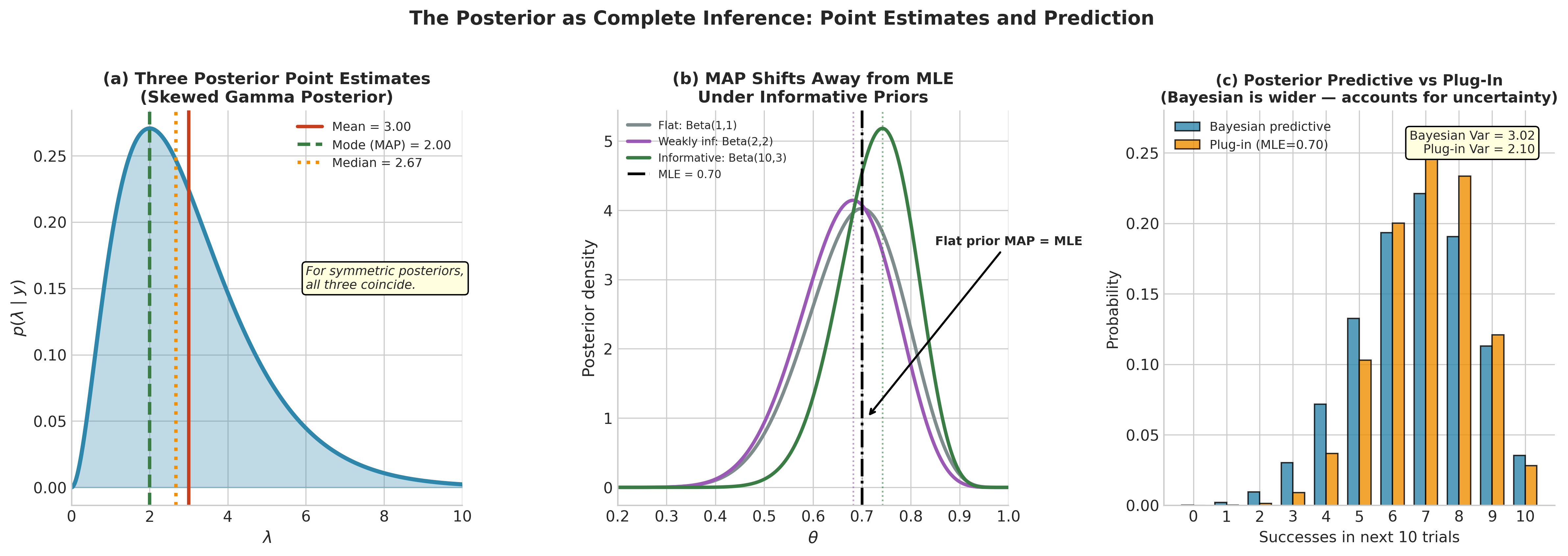
Fig. 178 Figure 5.7: The Posterior as Complete Inference. Panel (a) displays the three standard point estimates — mean, mode (MAP), and median — on a skewed Gamma posterior, illustrating how they diverge when the posterior is asymmetric. Panel (b) shows how the MAP estimate shifts away from the MLE as the prior becomes more informative: under a flat prior the MAP equals the MLE, but a Beta(10, 3) prior pulls the mode substantially leftward. Panel (c) compares the Bayesian posterior predictive distribution with the frequentist plug-in prediction for the next 10 trials; the Bayesian prediction is wider because it propagates parameter uncertainty through the integral \(p(\tilde{y} \mid y) = \int p(\tilde{y} \mid \theta) p(\theta \mid y) \, d\theta\), whereas the plug-in prediction conditions on a single point estimate.
The Likelihood Principle Revisited
In Section 1.1 Paradigms of Probability and Statistical Inference, we noted a philosophical distinction between frequentist and Bayesian inference regarding stopping rules. Here we make that distinction concrete with a computational demonstration that shows how identical data can produce different frequentist answers — but always the same Bayesian answer.
Setup. Consider two experimenters studying the same coin. Let \(\mathcal{M}_A\) and \(\mathcal{M}_B\) denote their respective sampling designs:
Experimenter A (design \(\mathcal{M}_A\)): flip the coin a fixed \(n = 12\) times. She observes \(k = 3\) heads. The sampling model is \(K \mid \theta, \mathcal{M}_A \sim \text{Binomial}(12, \theta)\).
Experimenter B (design \(\mathcal{M}_B\)): flip until \(r = 3\) heads are observed. She stops after \(n = 12\) flips. The sampling model is \(N \mid \theta, \mathcal{M}_B \sim \text{NegBin}(3, \theta)\).
The data — 3 heads in 12 flips — are identical. But the sampling models (and hence the sample spaces) differ, because the two experimenters had different intentions when they started the experiment.
Frequentist inference depends on the sample space. The \(p\)-values for testing \(H_0: \theta = 0.5\) depend on the set of all possible outcomes that could have been observed — outcomes determined by the experimental design, not the data. Under \(\mathcal{M}_A\), “more extreme” means 0, 1, 2, or 3 heads in 12 fixed flips. Under \(\mathcal{M}_B\), “more extreme” means needing 12 or more flips to accumulate 3 heads. These are different sample spaces, so the \(p\)-values differ:
Bayesian inference depends only on the likelihood. Both designs yield the same likelihood function up to a constant that does not depend on \(\theta\):
The combinatorial prefactors \(\binom{12}{3}\) and \(\binom{11}{2}\) differ, but they do not depend on \(\theta\) and therefore vanish in the proportional-to form. Since the posterior depends on the likelihood only through its dependence on \(\theta\), both experimenters obtain the same posterior regardless of the prior:
import numpy as np
from scipy import stats

k, n = 3, 12  # 3 heads in 12 flips

# --- Frequentist p-values differ by design ---
# Design M_A (Binomial): P(K <= 3 | n=12, theta=0.5)
p_value_A = stats.binom.cdf(k, n, 0.5)

# Design M_B (Neg. Binomial): P(failures >= 9 | r=3, theta=0.5)
# In 12 flips with 3 successes, there were 9 failures.
# SciPy's nbinom counts failures until r successes.
# P(X >= 9) = 1 - P(X <= 8)
p_value_B = 1 - stats.nbinom.cdf(8, 3, 0.5)

print("Frequentist p-values (test H0: theta = 0.5):")
print(f"  Design A (Binomial):      p = {p_value_A:.4f}")
print(f"  Design B (Neg. Binomial): p = {p_value_B:.4f}")

# --- Bayesian posteriors are identical ---
# Using Beta(1,1) = Uniform prior
alpha_post = 1 + k      # = 4
beta_post = 1 + (n - k)  # = 10
posterior = stats.beta(alpha_post, beta_post)

print(f"\nBayesian posterior (both designs):"
      f" Beta({alpha_post}, {beta_post})")
print(f"  Posterior mean:  {posterior.mean():.4f}")
print(f"  P(theta < 0.5 | data): {posterior.cdf(0.5):.4f}")
print(f"  95% credible interval: "
      f"({posterior.ppf(0.025):.4f}, {posterior.ppf(0.975):.4f})")
Frequentist p-values (test H0: theta = 0.5):
  Design A (Binomial):      p = 0.0730
  Design B (Neg. Binomial): p = 0.0327

Bayesian posterior (both designs): Beta(4, 10)
  Posterior mean:  0.2857
  P(theta < 0.5 | data): 0.9539
  95% credible interval: (0.0909, 0.5381)
This is the likelihood principle in action: inference should depend on the observed data through the likelihood function alone, not on the experimenter’s intentions or the stopping rule that determined how many observations were collected. Bayesian inference obeys the likelihood principle automatically — it follows as a mathematical consequence of conditioning on the observed data. Frequentist inference does not obey it in general — different sample spaces lead to different reference distributions and hence different \(p\)-values, even when the observed data are identical.
Whether the likelihood principle is a virtue (coherence, stopping-rule irrelevance) or a liability (ignoring relevant information about the design) depends on one’s inferential philosophy. What is indisputable is that the distinction has practical consequences: in sequential clinical trials, adaptive designs, and any experiment where the stopping time depends on the data, frequentist and Bayesian analyses may diverge. Understanding this divergence — and when it matters — is part of what it means to be a complete data scientist.
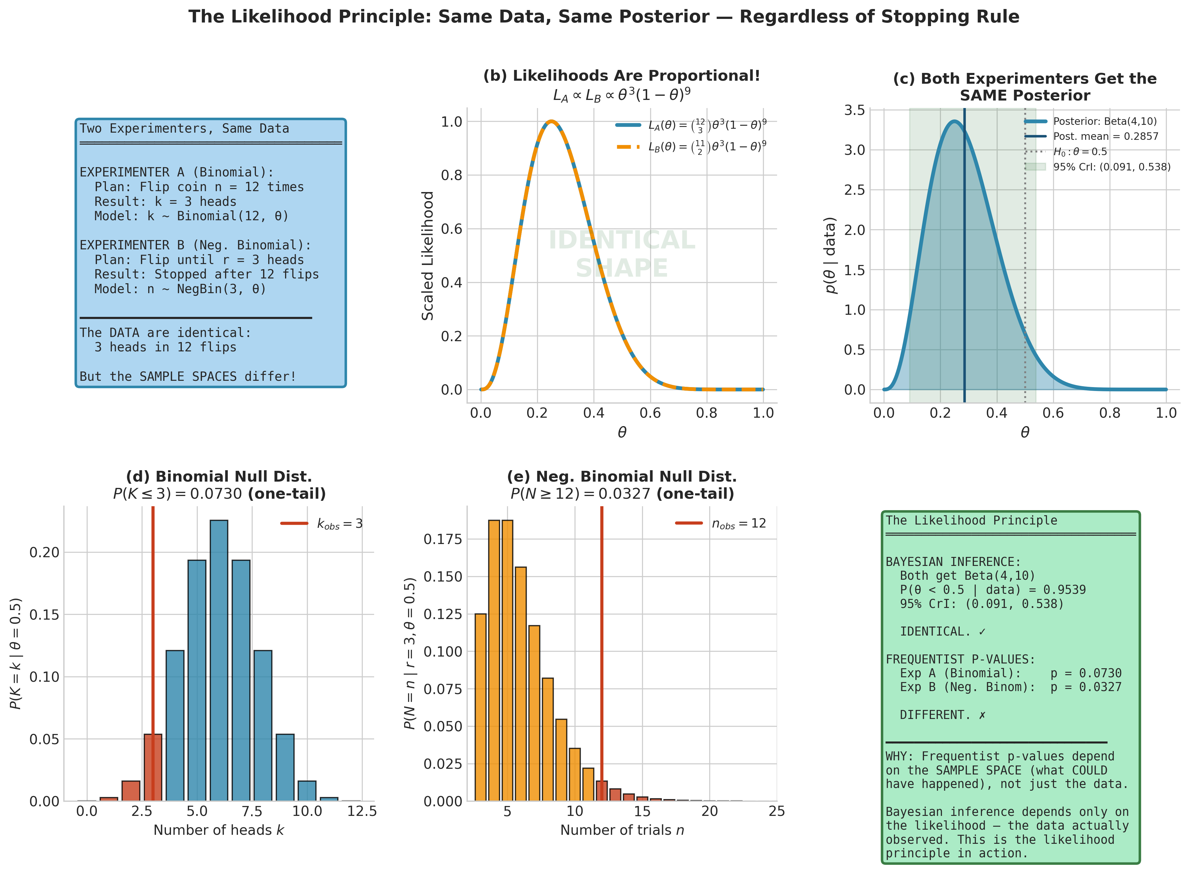
Fig. 179 Figure 5.8: The Likelihood Principle in Action. Two experimenters observe identical data (3 heads in 12 flips) under different sampling designs: \(\mathcal{M}_A\) fixes the number of trials (Binomial), \(\mathcal{M}_B\) fixes the number of successes (Negative Binomial). Panel (b) shows that both likelihoods \(L(\theta; \mathcal{M}_A)\) and \(L(\theta; \mathcal{M}_B)\) are proportional to \(\theta^3(1-\theta)^9\) — they differ only by a constant independent of \(\theta\). Panel (c) confirms that both designs yield the same Beta(4, 10) posterior. Panels (d–e) reveal the frequentist divergence: the null distributions under \(\mathcal{M}_A\) and \(\mathcal{M}_B\) differ because they depend on the sample space (what could have happened), not just the data observed. The Bayesian answer depends only on the likelihood.
Practical Considerations
Before moving to prior specification and conjugate analysis, we collect several practical guidelines for the methods introduced in this section.
When to use grid approximation. Grid approximation is the method of choice for one- or two-parameter problems where you want transparent, exact-to-machine-precision results. It is particularly useful for building intuition during the learning process (as in this chapter), for quick posterior exploration before committing to a full MCMC analysis, for problems where the posterior is known to be well-behaved (unimodal, bounded support), and for validating MCMC output by comparison on toy problems.
When grid approximation fails. Beyond two or three parameters, the curse of dimensionality makes grid approximation impractical. Even for low-dimensional problems, the grid must be fine enough to capture the posterior’s features — narrow modes, heavy tails, or multimodality can be missed by a coarse grid. Always check that your results are stable under grid refinement: double the number of grid points and widen the bounds, then verify that your posterior summaries do not change meaningfully. If they do, the grid is too coarse or too narrow.
Log-scale computation is mandatory. For any non-trivial dataset, the raw likelihood values will underflow to zero in floating-point arithmetic. Always work with log-likelihoods and log-priors, and use the log-sum-exp trick for normalization. This is not optional — it is a requirement for numerically correct results. The implementations provided above follow this practice throughout.
Choosing the grid range. The grid must span the region where the posterior has appreciable mass. A useful heuristic: start with the MLE (which you can find via Chapter 3’s methods) and extend the grid to \(\pm 4\) posterior standard deviations in each direction. For the first analysis, a preliminary run with a coarse grid can identify the relevant region, which can then be covered more finely.
Interpreting posterior summaries. The posterior mean, mode, and credible intervals are summaries of a distribution — they lose information relative to the full posterior. When the posterior is approximately normal (which happens in large samples by the Bernstein-von Mises theorem), these summaries capture the posterior well. When the posterior is multimodal, heavily skewed, or otherwise irregular, no single summary is adequate. In such cases, plot the full posterior density and interpret it visually before reducing to numerical summaries.
Common Pitfall ⚠️
A grid approximation that looks reasonable may be silently inaccurate if the grid does not extend far enough to cover the posterior tails. The symptom is subtle: because the approximation normalizes by the sum of grid values, a grid that truncates the tails will produce posterior probabilities that appear to sum to one — the normalization forces this — but the mean, variance, and quantiles will all be biased. Always verify stability: widen the grid bounds by 50% and check that your posterior summaries do not change. If the mean shifts or the variance decreases when you widen the grid, the original grid was too narrow.
Try It Yourself 🖥️
Modify the Beta-Binomial example above to explore how the prior-data balance shifts:
Keep the proportion \(k/n \approx 0.92\) (Curry’s free-throw rate) fixed but vary \(n\) from 5 to 500. Plot the posterior mean as a function of \(n\) alongside the prior mean and the MLE. At what sample size does the prior’s influence become negligible?
Fix \(n = 10, k = 8\) and try three priors: Beta(1, 1) (uniform), Beta(0.5, 0.5) (Jeffreys), and Beta(10, 10) (strong prior centered at 0.5). Compare the posterior means, modes, and 95% credible intervals. Which prior has the most influence, and why?
For the Michelson Normal mean-variance problem, increase the grid resolution from 200 × 200 to 500 × 500. Does the posterior change? How does the computation time scale?
Bringing It All Together
This section has established the operational framework for Bayesian inference, transforming the philosophical contrast from Chapter 1 into a working computational methodology. We began with the historical arc that brought Bayesian methods from Bayes’ 1763 essay through the Laplacian synthesis, the frequentist eclipse, and the MCMC revolution to their current status as a mature and widely used framework. That history is not incidental — it explains why the computational methods we develop in the remainder of this chapter were necessary and why they were so transformative.
We then laid out the three-step Bayesian workflow — specify a model, compute the posterior, evaluate fit — and distinguished it carefully from the frequentist pipeline developed across Chapters 3 and 4. The posterior distribution emerged as the central object of Bayesian inference. From it flow point estimates (mean, mode, median — each optimal under a different loss function), interval estimates (credible intervals, developed fully in Section 5.3 Posterior Inference: Credible Intervals and Hypothesis Assessment), and predictions (the posterior predictive distribution, which propagates parameter uncertainty automatically). We showed that the MLE is a special case of Bayesian MAP estimation under a flat prior, providing a precise bridge between the two inferential paradigms, and connected regularized regression to MAP estimation under specific prior families.
Grid approximation gave us a concrete computational strategy: discretize the parameter space, evaluate the unnormalized posterior at each grid point, normalize by the sum. It works beautifully for one- and two-parameter problems and makes the entire framework tangible. But the curse of dimensionality — the exponential growth of grid evaluations with parameter dimension — is a barrier that grid methods cannot overcome. This limitation motivates the progression that structures the rest of the chapter: conjugate analysis (Section 5.2 Prior Specification and Conjugate Analysis) avoids the grid entirely for special model families, while MCMC (Section 5.4 Markov Chains: The Mathematical Foundation of MCMC, Section 5.5 MCMC Algorithms: Metropolis-Hastings and Gibbs Sampling) provides a general-purpose solution that scales to models with hundreds or thousands of parameters.
The next section addresses the most distinctive — and most debated — element of the Bayesian framework: the prior distribution. Grid approximation in this section assumed we already had a prior in hand; Section 5.2 Prior Specification and Conjugate Analysis develops systematic strategies for choosing one, ranging from conjugate priors for computational convenience through weakly informative priors for regularization to informative priors that encode genuine scientific knowledge.
Key Takeaways 📝
Core concept: Bayesian inference treats parameters as random variables and conditions on observed data to obtain the posterior distribution \(p(\theta \mid y) \propto p(y \mid \theta) \, p(\theta)\). The posterior is the complete answer — point estimates, uncertainty quantification, and predictions all derive from it. The proportional-to form sidesteps the intractable normalizing constant that is the fundamental computational challenge of the framework. [LO 2, 4]
Computational insight: Grid approximation provides exact (to discretization error) posterior computation for low-dimensional problems, but its \(O(n_g^{\,d})\) cost makes it infeasible for \(d > 2\text{--}3\) parameters. Always work on the log scale and use the log-sum-exp trick for normalization. The curse of dimensionality motivates the MCMC methods developed in Sections 5.4–5.6. [LO 1, 4]
Practical application: Bayesian sequential updating — today’s posterior becomes tomorrow’s prior — enables online learning from streaming data without reprocessing history. The posterior mean compromises between prior and data, with the balance determined by relative precision: more data means less prior influence. [LO 2, 4]
Paradigm connections: The MLE is a special case of Bayesian MAP estimation under a flat prior, and regularized regression (ridge, LASSO) corresponds to MAP estimation under Normal and Laplace priors respectively — bridging the frequentist methods of Chapter 3 with the Bayesian framework. The likelihood principle guarantees that Bayesian inference depends on the data through the likelihood alone, not on the experimental design’s sample space. [LO 2]
Chapter 5.1 Exercises
These exercises develop your understanding of Bayesian foundations, from mechanical application of Bayes’ theorem through grid approximation to the conceptual distinctions between Bayesian and frequentist inference.
A Note on These Exercises
These exercises are designed to deepen your understanding of Bayesian foundations through hands-on derivation and implementation:
Exercise 1 reinforces the mechanics of Bayes’ theorem and discrete updating
Exercise 2 develops grid approximation skills and tests numerical stability
Exercise 3 explores the prior-data balance and shrinkage quantitatively
Exercise 4 connects Bayesian and frequentist inference through the MAP–MLE relationship
Exercise 5 examines the likelihood principle computationally
Complete solutions with derivations, code, output, and interpretation are provided. Work through the problems before checking solutions — the struggle builds understanding!
Exercise 1: Discrete Bayesian Updating
A factory produces widgets using three machines (A, B, C) with known defect rates: \(P(\text{defect} \mid A) = 0.01\), \(P(\text{defect} \mid B) = 0.05\), \(P(\text{defect} \mid C) = 0.10\). The machines produce 60%, 30%, and 10% of total output respectively.
A randomly selected widget is found to be defective. Compute the posterior probability that it came from each machine.
A second widget from the same batch is also defective. Update the posterior from part (a) using sequential updating. Verify that the result matches the batch update using both observations simultaneously.
How many consecutive defective widgets would be needed before \(P(C \mid \text{data}) > 0.5\)? Write a Python function to find this threshold.
Plot the posterior trajectories \(P(A \mid \text{data})\), \(P(B \mid \text{data})\), \(P(C \mid \text{data})\) as a function of the number of consecutive defective observations (from 0 to 10).
Solution
Part (a): Applying Bayes’ theorem with prior \(P(A) = 0.60, P(B) = 0.30, P(C) = 0.10\):
Similarly, \(P(B \mid D) \approx 0.484\) and \(P(C \mid D) \approx 0.323\). Despite producing only 10% of output, machine C’s high defect rate makes it the second most likely source.
Part (b): Using \(P(\cdot \mid D)\) from part (a) as the new prior and updating with a second defective:
Normalizing: \(P(A \mid D,D) \approx 0.034\), \(P(B \mid D,D) \approx 0.420\), \(P(C \mid D,D) \approx 0.560\). Batch update: multiply prior by \((\text{defect rate})^2\) for each machine and normalize — yields the same result.
Parts (c–d):
import numpy as np

prior = np.array([0.60, 0.30, 0.10])
defect_rates = np.array([0.01, 0.05, 0.10])

post = prior.copy()
for n_defects in range(1, 11):
    unnorm = defect_rates * post
    post = unnorm / unnorm.sum()
    if post[2] > 0.5 and n_defects == np.argmax(post[2] > 0.5) + 1:
        print(f"After {n_defects} defects: P(C|data) = {post[2]:.4f}")
    print(f"n={n_defects}: P(A)={post[0]:.4f}, P(B)={post[1]:.4f}, P(C)={post[2]:.4f}")
After 2 consecutive defective widgets, \(P(C \mid \text{data}) > 0.5\).
Exercise 2: Grid Approximation with Log-Scale Computation
Consider \(n = 100\) observations from an Exponential(\(\lambda\)) distribution with sample mean \(\bar{x} = 2.3\). Use a Gamma(2, 0.5) prior on \(\lambda\).
Derive the conjugate posterior analytically (the Gamma-Exponential conjugate pair).
Implement a grid approximation with \(n_g = 500\) points on \([0.1, 2.0]\) using log-scale computation. Compare the grid posterior mean, mode, and 95% credible interval with the exact conjugate values.
Demonstrate why log-scale computation is essential: repeat part (b) without log-scale (i.e., computing
prior * likelihooddirectly). At what sample size does the naive computation producenanor0.0values?Investigate grid range sensitivity: repeat the grid approximation with range \([0.1, 1.0]\) (too narrow) and \([0.001, 10.0]\) (too wide). How do the posterior summaries change, and what diagnostic would detect the problem?
Solution
Part (a): For Exponential data with sufficient statistic \(\sum x_i = n\bar{x} = 230\), the Gamma(\(\alpha, \beta\)) conjugate update yields:
Posterior mean \(= 102 / 230.5 \approx 0.4425\), mode \(= 101/230.5 \approx 0.4382\).
Part (b):
import numpy as np
from scipy import stats
from scipy.special import logsumexp

n, xbar = 100, 2.3
alpha_prior, beta_prior = 2, 0.5
alpha_post = alpha_prior + n  # 102
beta_post = beta_prior + n * xbar  # 230.5

n_g = 500
lam_grid = np.linspace(0.1, 2.0, n_g)
log_prior = stats.gamma.logpdf(lam_grid, a=alpha_prior, scale=1/beta_prior)
log_lik = -n * lam_grid * xbar + n * np.log(lam_grid)  # sum of log-exponential
log_unnorm = log_prior + log_lik
log_post = log_unnorm - logsumexp(log_unnorm)
post_w = np.exp(log_post)
post_w /= post_w.sum()

grid_mean = np.sum(lam_grid * post_w)
exact = stats.gamma(a=alpha_post, scale=1/beta_post)
print(f"Grid mean: {grid_mean:.4f}, Exact: {exact.mean():.4f}")
Part (c): Without log-scale, prior * likelihood underflows to 0.0 for all grid points once \(n \gtrsim 20\), because \(e^{-\lambda \cdot n\bar{x}}\) is astronomically small for most \(\lambda\) values.
Part (d): A too-narrow grid truncates the tails: the posterior weights at the boundaries are nonzero, indicating probability mass is being cut off. Diagnostic: check that the boundary weights are effectively zero (e.g., less than \(10^{-6}\) of the peak).
Exercise 3: Quantifying the Prior-Data Balance
Using the Beta-Binomial conjugate model with \(k\) successes in \(n\) trials and a Beta(\(\alpha_0, \beta_0\)) prior:
Show algebraically that the posterior mean can be written as a weighted average:
\[\mathbb{E}[\theta \mid k, n] = w \cdot \frac{k}{n} + (1 - w) \cdot \frac{\alpha_0}{\alpha_0 + \beta_0}\]where \(w = n / (n + \alpha_0 + \beta_0)\). Interpret the weight \(w\) in terms of “effective sample sizes.”
For the vaccine trial (\(n = 50, k = 38\)) with a Beta(2, 2) prior, compute \(w\) and verify numerically that the weighted-average formula reproduces the exact posterior mean.
How large must \(n\) be for the data to contribute at least 99% of the weight (i.e., \(w \geq 0.99\))? How does this depend on the prior strength \(\alpha_0 + \beta_0\)?
Generate a plot showing the posterior mean as a function of \(n\) (from 1 to 500, holding \(k/n = 0.76\) fixed) for three priors: Beta(1, 1), Beta(10, 10), and Beta(50, 50). Annotate where \(w = 0.5, 0.9, 0.99\) for each prior.
Solution
Part (a): The Beta(\(\alpha_0 + k, \beta_0 + n - k\)) posterior has mean:
The weight \(w = n / (n + \alpha_0 + \beta_0)\) is the ratio of the data “sample size” \(n\) to the total effective sample size \(n + (\alpha_0 + \beta_0)\), where \(\alpha_0 + \beta_0\) is the prior’s effective sample size (number of prior pseudo-observations).
Part (b): With \(n = 50\), \(\alpha_0 + \beta_0 = 4\): \(w = 50/54 \approx 0.926\). Check: \(0.926 \times 0.76 + 0.074 \times 0.50 = 0.7038 + 0.0370 = 0.7407\), matching \(40/54\).
Part (c): \(w \geq 0.99\) requires \(n \geq 99(\alpha_0 + \beta_0)\). For Beta(2, 2): \(n \geq 396\). For Beta(50, 50): \(n \geq 9{,}900\).
Exercise 4: MAP, MLE, and Regularization
For a Normal(\(\mu\), \(\sigma^2 = 1\)) model with known variance and a Normal(\(0, \tau^2\)) prior on \(\mu\), show that the MAP estimate given data \(x_1, \ldots, x_n\) is:
\[\hat{\mu}_{\text{MAP}} = \frac{n\bar{x}/\sigma^2}{n/\sigma^2 + 1/\tau^2}\]and that this is identical to the ridge regression estimator with penalty \(\lambda_{\text{ridge}} = \sigma^2 / \tau^2\).
Show that as \(\tau \to \infty\) (flat prior), \(\hat{\mu}_{\text{MAP}} \to \hat{\mu}_{\text{MLE}} = \bar{x}\), and as \(\tau \to 0\) (infinitely strong prior at 0), \(\hat{\mu}_{\text{MAP}} \to 0\).
Implement a simulation: generate \(n = 20\) observations from Normal(\(\mu = 3, \sigma^2 = 1\)). Compute the MLE and the MAP estimate for \(\tau^2 \in \{0.1, 0.5, 1, 5, 50\}\). Plot all estimates on a number line with the true \(\mu\) marked. Discuss the bias-variance tradeoff.
Solution
Part (a): The log posterior is \(-\frac{1}{2\sigma^2}\sum(x_i - \mu)^2 - \frac{\mu^2}{2\tau^2} + \text{const}\). Taking the derivative and setting to zero:
This is precisely the ridge regression solution with \(\lambda = \sigma^2/\tau^2\). A tight prior (\(\tau\) small) corresponds to strong regularization (\(\lambda\) large).
Part (b): As \(\tau \to \infty\), \(1/\tau^2 \to 0\), so the denominator \(\to n/\sigma^2\) and \(\hat{\mu}_{\text{MAP}} \to \bar{x}\). As \(\tau \to 0\), \(1/\tau^2 \to \infty\) dominates, so \(\hat{\mu}_{\text{MAP}} \to 0\).
Exercise 5: The Likelihood Principle in Practice
Verify the likelihood principle example from the text computationally: for \(k = 3\) heads in \(n = 12\) flips, compute the Binomial and Negative Binomial \(p\)-values for \(H_0: \theta = 0.5\) and confirm they differ, while the Bayesian posterior (under a Uniform prior) is identical.
Now consider a clinical trial where a drug is tested until either \(r = 5\) successes or \(n_{\max} = 30\) patients have been treated. In the trial, the 5th success occurs at patient 28. Compute the posterior under a Beta(1, 1) prior. Explain why a frequentist analysis of this design is more complex (what is the correct reference distribution?), whereas the Bayesian analysis is straightforward.
Write a simulation that compares the frequentist Type I error rate and the Bayesian posterior \(P(\theta < 0.5 \mid \text{data})\) across 1,000 replicated experiments under \(H_0: \theta = 0.5\), using the stopping rule from part (b). Does the Bayesian analysis maintain its nominal properties?
Solution
Part (a):
from scipy import stats

k, n = 3, 12
# Binomial: P(K <= 3 | n=12, p=0.5)
p_binom = stats.binom.cdf(k, n, 0.5)
# NegBinom: P(failures >= 9 | r=3, p=0.5)
p_negbin = 1 - stats.nbinom.cdf(n - k - 1, k, 0.5)
# Bayesian: Beta(1+3, 1+9) = Beta(4, 10)
posterior = stats.beta(4, 10)

print(f"Binomial p-value:     {p_binom:.4f}")
print(f"Neg. Binomial p-value: {p_negbin:.4f}")
print(f"Posterior mean:        {posterior.mean():.4f}")
The \(p\)-values differ (0.0730 for the Binomial design vs. 0.0327 for the Negative-Binomial design) even though both experiments observed the same data, because the two sampling plans define different sample spaces. The posterior is identical regardless of the sampling plan.
Part (b): With 5 successes in 28 patients: posterior is Beta(\(1 + 5, 1 + 23\)) = Beta(6, 24). The Bayesian analysis does not depend on the stopping rule. The frequentist analysis requires computing the sampling distribution under a composite stopping rule (stop at \(r = 5\) or \(n = 30\), whichever comes first), which has no standard form.