Section 4.7 Bootstrap Confidence Intervals: Advanced Methods (Optional)
Optional Section — Self-Study
This section is not covered in class; it is kept as a self-study reference. Nothing later in the course depends on it: Chapter 5 quantifies uncertainty with posterior credible intervals, and every bootstrap confidence interval in Chapter 6 uses the percentile method of Section 4.3. Read this section when you need intervals with better small-sample coverage than the percentile method delivers: the studentized (bootstrap-t) and bias-corrected and accelerated (BCa) constructions, why they are second-order accurate, and how to control Monte Carlo error from a finite number of bootstrap replicates. (It draws on the leave-one-out values of the optional Section 4.5, restated where used.)
In Section 4.3, we introduced three basic bootstrap confidence interval methods: the percentile interval, the basic (pivotal) interval, and the normal approximation. These methods are intuitive, easy to implement, and often adequate for exploratory analysis. However, they share a fundamental limitation: their coverage accuracy degrades in predictable ways when the bootstrap distribution is skewed, when the estimator is biased, or when the standard error varies with the parameter value. This section develops advanced bootstrap interval methods—the studentized (bootstrap-t) interval and the bias-corrected and accelerated (BCa) interval—that achieve improved coverage accuracy by addressing these sources of error systematically.
The distinction between “first-order” and “second-order” accurate methods has profound practical consequences. For a nominal 95% confidence interval at moderate sample sizes (often n ≈ 30–100), first order methods can exhibit noticeable undercoverage in skewed or biased settings, especially for one sided inference; second order methods typically reduce this error substantially. The magnitude depends on the functional and the underlying distribution. Throughout this section, we build on tools developed earlier: the jackknife estimates \(\hat{\theta}_{(-i)}\) from Section 4.5 are essential for computing the BCa acceleration constant, and the bootstrap distribution \(\{\hat{\theta}^*_b\}\) from Section 4.3 remains our primary computational object. We also address a practical concern that pervades all bootstrap inference: Monte Carlo error from using finitely many bootstrap replicates \(B\). Understanding and controlling this error is essential for reporting results responsibly.
Road Map 🧭
Understand: Why percentile and basic intervals have coverage deficiencies, and how Edgeworth expansions characterize coverage error rates
Develop: The studentized bootstrap and BCa intervals as two routes to second-order accuracy
Implement: Complete Python implementations with proper numerical handling of edge cases
Evaluate: Diagnostic tools for method selection and Monte Carlo error quantification
Why Advanced Methods?
Before developing sophisticated interval constructions, we must understand why simple methods fall short. The answer lies in the structure of sampling distributions and how bootstrap approximations inherit—or fail to correct—systematic errors.
The Coverage Probability Target
A confidence interval procedure produces a random interval \([\hat{L}_n, \hat{U}_n]\) that depends on the observed data \(X_1, \ldots, X_n\). The coverage probability is the chance that this random interval contains the true parameter:
where the probability is taken over the sampling distribution of the data under the true distribution \(F\). For a nominal \((1-\alpha)\) confidence interval, we want \(C_n(F) = 1 - \alpha\) for all \(F\) in some class of interest. In practice, we settle for \(C_n(F) \approx 1 - \alpha\) when \(n\) is large.
The coverage error is the difference between actual and nominal coverage:
A positive coverage error means the interval is conservative (over-covers); a negative error means the interval is liberal (under-covers). Neither is desirable, but under-coverage—where the actual coverage falls below the target in (117)—is typically more problematic since it leads to overconfident inference.
Coverage Is Not Random
A common confusion: coverage probability \(C_n(F)\) is a fixed number for given \(F\) and \(n\), not a random variable. Once we specify the data-generating distribution \(F\), the coverage probability is determined by integrating over all possible samples. The big-\(O\) notation we use below describes how this fixed quantity behaves as \(n \to \infty\).
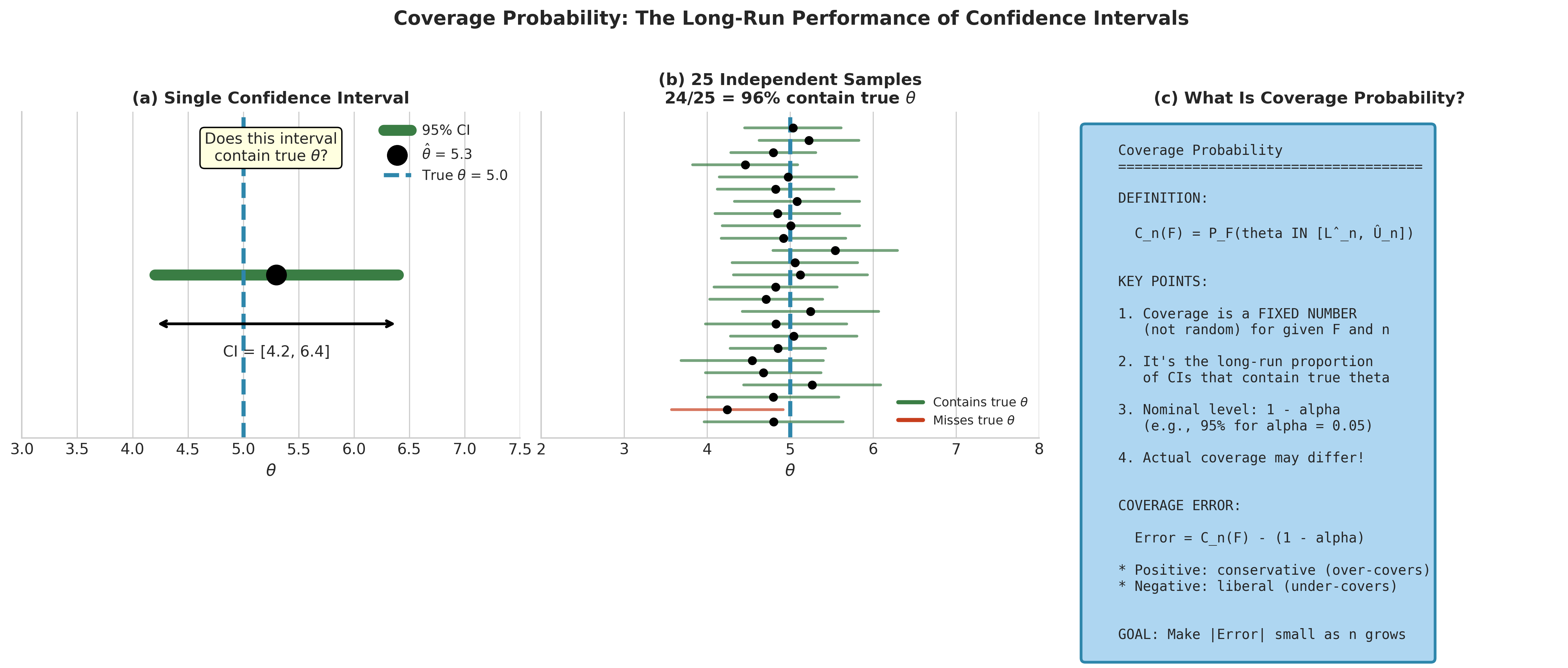
Fig. 156 Figure 4.7.1: Coverage probability visualized. (a) A single confidence interval either contains (✓) or misses (✗) the true parameter—we cannot know which from the data alone. (b) Over many repetitions from the same population, the coverage probability is the long-run proportion of intervals that contain the truth. (c) The formal definition: coverage is the probability that the random interval captures the fixed but unknown parameter.
Edgeworth Expansions and Coverage Error Rates
The key theoretical tool for understanding coverage error is the Edgeworth expansion, which refines the Central Limit Theorem by providing correction terms that capture departures from normality at finite sample sizes. (This section uses asymptotic \(O(\cdot)\) notation extensively; see Appendix C for the formal definitions.)
For a standardized statistic \(Z_n = \sqrt{n}(\hat{\theta} - \theta)/\sigma\), the distribution function admits an expansion of the form:
where \(\Phi\) and \(\phi\) are the standard normal CDF and PDF, and \(p_1, p_2\) are polynomials whose coefficients depend on the moments of the underlying distribution. Crucially:
\(p_1(z)\) is an odd polynomial (involving skewness)
\(p_2(z)\) is an even polynomial (involving kurtosis and skewness squared)
This structure has profound implications for confidence interval coverage.
One-sided intervals: For a one-sided interval of the form \((-\infty, \hat{\theta} + z_{1-\alpha} \cdot \hat{\sigma}/\sqrt{n}]\), the coverage error is dominated by the \(p_1\) term:
The leading error term is \(O(n^{-1/2})\), which can be substantial for moderate \(n\).
Two-sided intervals: For symmetric two-sided intervals, the odd polynomial \(p_1\) contributes errors of opposite sign at the two endpoints, and these partially cancel:
The leading error is \(O(n^{-1})\), an order of magnitude smaller than for one-sided intervals.
This asymmetry between one-sided and two-sided coverage is a fundamental feature of confidence interval theory. Methods that achieve \(O(n^{-1})\) coverage error for both one-sided and two-sided intervals are called second-order accurate.
Note: symmetric two-sided intervals can achieve \(O(n^{-1})\) error via cancellation even when the underlying one-sided error remains \(O(n^{-1/2})\); “second-order accurate” here refers to constructions that remove the \(O(n^{-1/2})\) term for one-sided coverage as well.
Why Percentile and Basic Intervals Are First-Order
The percentile interval \([Q_{\alpha/2}(\hat{\theta}^*), Q_{1-\alpha/2}(\hat{\theta}^*)]\) uses quantiles of the bootstrap distribution directly. While this captures the shape of the sampling distribution, it inherits systematic errors:
Bias drift: If \(\mathbb{E}[\hat{\theta}] \neq \theta\), the bootstrap distribution is centered at \(\hat{\theta}\) rather than \(\theta\), causing the interval to drift.
Skewness mismatch: The bootstrap distribution of \(\hat{\theta}^* - \hat{\theta}\) estimates the distribution of \(\hat{\theta} - \theta\), but the quantiles don’t align perfectly when these distributions are skewed.
The basic interval \([2\hat{\theta} - Q_{1-\alpha/2}(\hat{\theta}^*), 2\hat{\theta} - Q_{\alpha/2}(\hat{\theta}^*)]\) partially corrects the bias drift by reflecting quantiles about \(\hat{\theta}\), but it doesn’t address skewness.
For smooth functionals under standard regularity conditions, one sided percentile and basic intervals typically have coverage error \(O(n^{-1/2})\). For symmetric two-sided intervals, odd order terms partially cancel, often yielding \(O(n^{-1})\) coverage error. This is why these methods often perform reasonably for two-sided intervals but can have serious coverage problems for one-sided intervals.
The Goal of Advanced Methods
Advanced bootstrap interval methods aim to achieve \(O(n^{-1})\) coverage error for both one-sided and two-sided intervals. There are two main approaches:
Studentization: Pivot by an estimated standard error, transforming the problem so that the leading odd term in the Edgeworth expansion vanishes.
Transformation correction (BCa): Find quantile adjustments that automatically account for bias and skewness, achieving transformation invariance.
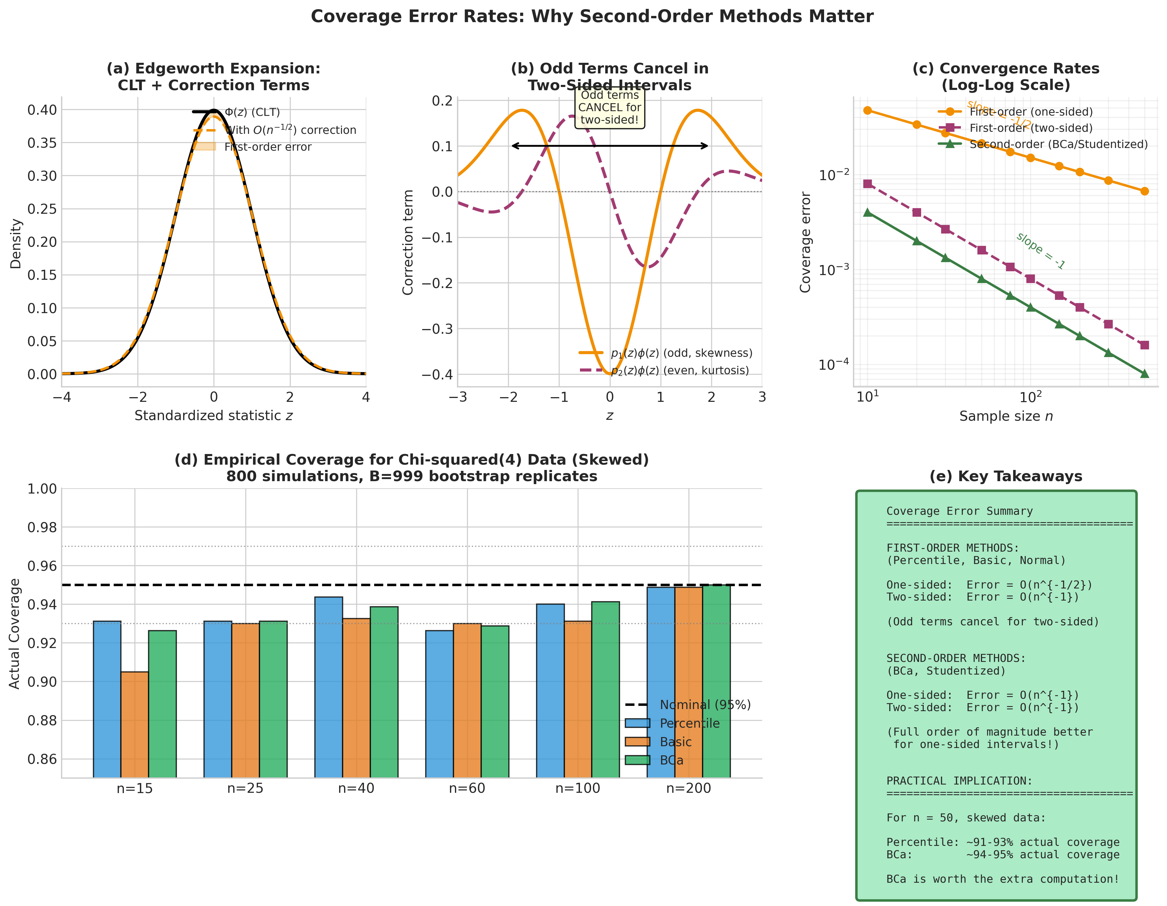
Fig. 157 Figure 4.7.2: Coverage error rates from Edgeworth expansions. (a) The first correction term \(p_1(z)\phi(z)\) is an odd function, contributing \(O(n^{-1/2})\) error for one-sided intervals but canceling for two-sided intervals. (b) Comparison of coverage error magnitude: first-order methods (Percentile, Basic, BC) vs second-order methods (BCa, Studentized). (c) Simulation study confirming the theoretical rates—second-order methods approach nominal coverage faster.
Practical Implications
To make these abstract rates concrete, consider the following rough guide for nominal 95% two-sided intervals:
\(n\) |
Normal Approx |
Percentile |
BCa |
Studentized |
|---|---|---|---|---|
20 |
88–92% |
89–93% |
93–95% |
93–95% |
50 |
92–94% |
92–94% |
94–95% |
94–95% |
100 |
93–95% |
93–95% |
94.5–95% |
94.5–95% |
500 |
94.5–95% |
94.5–95% |
~95% |
~95% |
These are illustrative ranges; actual coverage depends on the statistic and underlying distribution. The key message: for moderate sample sizes, the difference between first-order and second-order methods can be the difference between 91% and 94% actual coverage for a nominal 95% interval.
The Studentized (Bootstrap-t) Interval
The studentized bootstrap, also called the bootstrap-t method, extends the classical Student’s t approach to general statistics. The key insight is that dividing by an estimated standard error creates a more pivotal quantity—one whose distribution depends less on unknown parameters—and this pivotality translates directly into improved coverage accuracy.
From Student’s t to Bootstrap-t
Recall the classical setting: for iid observations \(X_1, \ldots, X_n\) from a normal distribution with unknown mean \(\mu\) and variance \(\sigma^2\), the pivot
follows a \(t_{n-1}\) distribution regardless of the values of \(\mu\) and \(\sigma^2\). This pivotality means that \(t\)-based intervals have exact coverage under normality.
For a general statistic \(\hat{\theta}\) estimating \(\theta\), we can form an analogous studentized quantity:
where \(\hat{\sigma}\) is an estimate of the standard error of \(\hat{\theta}\). Unlike the normal-theory case, \(T\) doesn’t have a known distribution—but the bootstrap can estimate it.
The Bootstrap-t Algorithm
The bootstrap-t method estimates the distribution of \(T\) by computing its bootstrap analog \(T^*\) across many resamples.
Algorithm: Studentized Bootstrap Confidence Interval
Input: Data X₁,...,Xₙ; statistic T; SE estimator; replicates B; level α
Output: (1-α) studentized bootstrap CI

1. Compute θ̂ = T(X₁,...,Xₙ) and σ̂ = SE(X₁,...,Xₙ)
2. For b = 1,...,B:
   a. Draw bootstrap sample X*₁,...,X*ₙ (with replacement)
   b. Compute θ̂*_b = T(X*₁,...,X*ₙ)
   c. Compute σ̂*_b = SE(X*₁,...,X*ₙ)  [using same SE method]
   d. Compute t*_b = (θ̂*_b - θ̂) / σ̂*_b
3. Let q*_{α/2} and q*_{1-α/2} be the α/2 and (1-α/2) quantiles of {t*_b}
4. Return CI: [θ̂ - σ̂ · q*_{1-α/2}, θ̂ - σ̂ · q*_{α/2}]
The crucial step is computing \(\hat{\sigma}^*_b\) within each bootstrap sample. This allows the bootstrap distribution of \(T^*\) to capture how the studentized statistic varies, including any relationship between \(\hat{\theta}\) and its standard error.
Why the Quantiles Reverse
The interval formula subtracts \(q^*_{1-\alpha/2}\) to get the lower bound and \(q^*_{\alpha/2}\) to get the upper bound. This reversal arises from inverting the pivot relationship:
Solving for \(\theta\):
Why Studentization Achieves Second-Order Accuracy
The theoretical advantage of studentization can be understood through Edgeworth expansions. For a non-studentized statistic \(\sqrt{n}(\hat{\theta} - \theta)/\sigma\), the leading correction term \(p_1(z)\) in (118) is an odd polynomial that contributes \(O(n^{-1/2})\) error to one-sided coverage.
For the studentized statistic \(T = \sqrt{n}(\hat{\theta} - \theta)/\hat{\sigma}\), the Edgeworth expansion has the form:
The \(n^{-1/2}\) term with an odd polynomial is absent (or its coefficient is zero). This occurs because the studentized pivot (119) absorbs the leading skewness correction into the variance estimation. The technical conditions for this improvement, established by Hall (1988, 1992), include:
Finite fourth moments: \(\mathbb{E}|X|^{4+\delta} < \infty\) for some \(\delta > 0\)
Cramér’s condition on the characteristic function (ensuring non-lattice distributions)
Sufficient smoothness of \(\hat{\theta}\) as a function of sample moments
Consistent variance estimation: \(\hat{\sigma}/\sigma \xrightarrow{p} 1\)
Under these conditions, the studentized bootstrap achieves coverage error \(O(n^{-1})\) for both one-sided and two-sided intervals—a full order of magnitude improvement over percentile and basic methods for one-sided intervals.
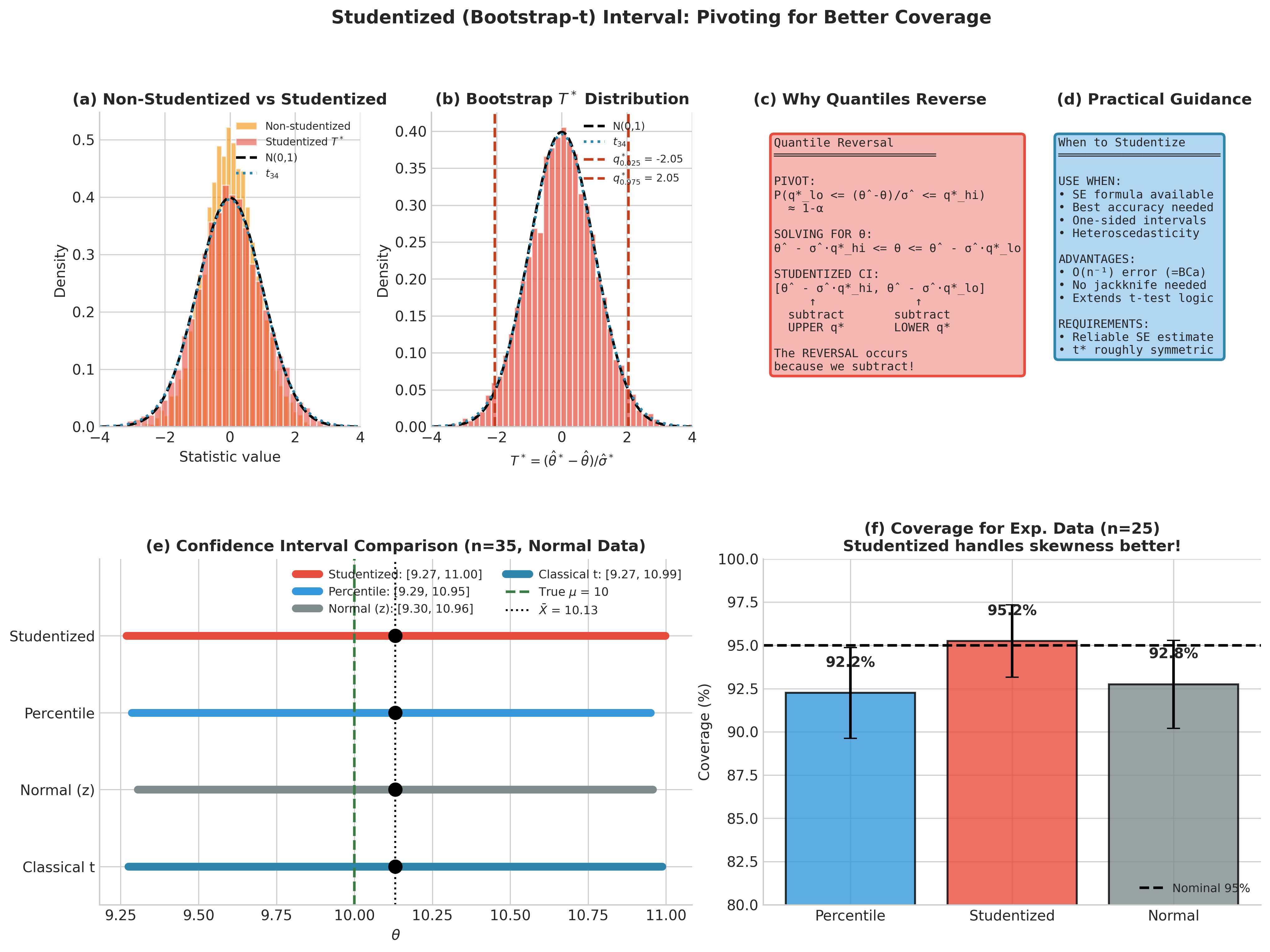
Fig. 158 Figure 4.7.3: The studentized (bootstrap-t) method. (a) Comparison of non-studentized vs studentized bootstrap statistics—studentization produces a distribution closer to the reference \(t\) distribution. (b) The bootstrap \(T^*\) distribution with quantiles used for interval construction. (c-d) Explanation of quantile reversal and practical guidance. (e) Confidence interval comparison across methods for normal data. (f) Coverage simulation on exponential data demonstrating studentized method’s advantage for skewed distributions.
Methods for Estimating SE Within Bootstrap Samples
The practical challenge of bootstrap-t is computing \(\hat{\sigma}^*_b\) for each bootstrap sample. Several approaches exist, with different trade-offs:
Option 1: Analytical (Plug-in) SE
When a closed-form standard error formula exists, apply it to each bootstrap sample.
Example: For the sample mean, \(\hat{\sigma}^*_b = s^*_b/\sqrt{n}\) where \(s^*_b\) is the sample standard deviation of the bootstrap sample.
Example: For OLS regression with homoscedastic errors, use \(\hat{\sigma}^*_{\hat{\beta}} = \hat{\sigma}^*_\epsilon \sqrt{(X^{*\top}X^*)^{-1}_{jj}}\).
Advantages: Fast (\(O(B)\) total complexity), exact within model assumptions.
Disadvantages: Requires known formula; may be inaccurate under model misspecification (e.g., heteroscedasticity).
Option 2: Sandwich (Robust) SE
For regression problems, use heteroscedasticity-consistent standard errors within each bootstrap sample:
This provides robustness to heteroscedasticity while maintaining analytical tractability.
Option 3: Jackknife SE Within Bootstrap Samples
Use the delete-1 jackknife (from Section 4.5) to estimate \(\hat{\sigma}^*_b\):
where \(\hat{\theta}^*_{b,(-i)}\) is the statistic computed on bootstrap sample \(b\) with observation \(i\) removed.
Advantages: Works for any statistic; no formula needed.
Disadvantages: Cost is \(O(B \cdot n)\) statistic evaluations; may be unstable for non-smooth statistics.
Option 4: Nested Bootstrap
For each outer bootstrap sample \(b\), draw \(M\) inner bootstrap samples and compute \(\hat{\sigma}^*_b\) as the standard deviation of the inner bootstrap estimates.
Advantages: Most general; works for any statistic.
Disadvantages: Cost is \(O(B \cdot M)\) statistic evaluations; can be prohibitive for expensive statistics.
Practical Guidance: Use analytical or sandwich SE when available and trustworthy. Use jackknife SE as a general-purpose fallback. Reserve nested bootstrap for non-smooth statistics where jackknife is unreliable.
Python Implementation
import numpy as np
from scipy import stats

def studentized_bootstrap_ci(data, statistic, se_function, alpha=0.05,
                              B=5000, seed=None):
    """
    Compute studentized (bootstrap-t) confidence interval.

    Parameters
    ----------
    data : array_like
        Original data (1D array for simple case).
    statistic : callable
        Function computing the statistic: statistic(data) -> float.
    se_function : callable
        Function computing SE estimate: se_function(data) -> float.
    alpha : float
        Significance level (default 0.05 for 95% CI).
    B : int
        Number of bootstrap replicates.
    seed : int, optional
        Random seed for reproducibility.

    Returns
    -------
    ci : tuple
        (lower, upper) confidence bounds.
    theta_hat : float
        Original point estimate.
    info : dict
        Additional information including t* distribution.
    """
    rng = np.random.default_rng(seed)
    data = np.asarray(data)
    n = len(data)

    # Original estimates
    theta_hat = statistic(data)
    se_hat = se_function(data)

    # Bootstrap
    t_star = np.empty(B)
    theta_star = np.empty(B)

    for b in range(B):
        # Resample with replacement
        idx = rng.integers(0, n, size=n)
        data_star = data[idx]

        # Compute statistic and SE on bootstrap sample
        theta_star[b] = statistic(data_star)
        se_star = se_function(data_star)

        # Studentized statistic (guard against zero SE)
        if se_star > 1e-10:
            t_star[b] = (theta_star[b] - theta_hat) / se_star
        else:
            t_star[b] = np.nan  # Degenerate case

    # Quantiles of t* distribution
    q_lo = np.quantile(t_star, alpha / 2)
    q_hi = np.quantile(t_star, 1 - alpha / 2)

    # Confidence interval (note the reversal)
    ci_lower = theta_hat - se_hat * q_hi
    ci_upper = theta_hat - se_hat * q_lo

    info = {
        't_star': t_star,
        'theta_star': theta_star,
        'se_hat': se_hat,
        'q_lo': q_lo,
        'q_hi': q_hi
    }

    return (ci_lower, ci_upper), theta_hat, info


def jackknife_se(data, statistic):
    """
    Compute jackknife standard error for use in studentized bootstrap.

    Parameters
    ----------
    data : array_like
        Data array.
    statistic : callable
        Function computing the statistic.

    Returns
    -------
    se : float
        Jackknife standard error estimate.
    """
    data = np.asarray(data)
    n = len(data)

    # Leave-one-out estimates
    theta_jack = np.empty(n)
    for i in range(n):
        data_minus_i = np.delete(data, i)
        theta_jack[i] = statistic(data_minus_i)

    # Jackknife SE formula
    theta_bar = theta_jack.mean()
    se = np.sqrt((n - 1) / n * np.sum((theta_jack - theta_bar)**2))

    return se
Example 💡 Studentized Bootstrap for Correlation Coefficient
Given: Paired observations \((X_i, Y_i)\) for \(i = 1, \ldots, 30\) from a bivariate distribution.
Find: A 95% confidence interval for the population correlation \(\rho\).
Challenge: The sampling distribution of \(\hat{\rho}\) is skewed, especially when \(|\rho|\) is large, and the standard error depends on \(\rho\) itself.
Python implementation:
import numpy as np
from scipy import stats

# Generate example data with true correlation rho = 0.7
rng = np.random.default_rng(42)
n = 30
rho_true = 0.7

# Generate from a bivariate normal
mean = [0, 0]
cov = [[1, rho_true], [rho_true, 1]]
data = rng.multivariate_normal(mean, cov, size=n)
x, y = data[:, 0], data[:, 1]

# Combine into single array for resampling (pairs bootstrap)
xy = np.column_stack([x, y])

def correlation(xy_data):
    """Compute Pearson correlation on the r scale."""
    return np.corrcoef(xy_data[:, 0], xy_data[:, 1])[0, 1]

def correlation_fisher_z(xy_data):
    """Compute Fisher z = atanh(r), where r is Pearson correlation."""
    r = correlation(xy_data)
    # Clip to avoid infinities at |r| = 1 due to finite precision
    r = np.clip(r, -0.999999999, 0.999999999)
    return np.arctanh(r)

def correlation_se_fisher_z(xy_data):
    """SE of Fisher z: Var(z) ≈ 1/(n-3)."""
    n_local = len(xy_data)
    return 1 / np.sqrt(n_local - 3) if n_local > 3 else np.nan

# Studentized bootstrap CI on Fisher z scale, then transform back to r scale
ci_stud_z, z_hat, info = studentized_bootstrap_ci(
    xy,
    correlation_fisher_z,
    correlation_se_fisher_z,
    alpha=0.05,
    B=10000,
    seed=123
)

ci_stud_r = (np.tanh(ci_stud_z[0]), np.tanh(ci_stud_z[1]))
r_hat = correlation(xy)

print(f"Sample correlation (r): {r_hat:.4f}")
print(f"True correlation:       {rho_true}")
print(f"95% Studentized CI (r): [{ci_stud_r[0]:.4f}, {ci_stud_r[1]:.4f}]")

# Compare with percentile CI on r scale
theta_star_z = info["theta_star"]
theta_star_r = np.tanh(theta_star_z)
ci_perc_r = (np.quantile(theta_star_r, 0.025), np.quantile(theta_star_r, 0.975))
print(f"95% Percentile CI (r):  [{ci_perc_r[0]:.4f}, {ci_perc_r[1]:.4f}]")
Result: The studentized interval properly accounts for the asymmetric sampling distribution of the correlation coefficient, while the percentile interval may have coverage issues, particularly when the true correlation is far from zero.
Diagnostics for Studentized Bootstrap
Before trusting a studentized bootstrap interval, examine the distribution of \(t^*\):
Shape: The \(t^*\) distribution should be unimodal and roughly symmetric. Compare with a standard normal or \(t\) distribution.
Outliers: Extreme \(t^*\) values often indicate bootstrap samples where \(\hat{\sigma}^*_b \approx 0\). These can distort quantiles.
Stability: Verify that the \(t^*\) quantiles stabilize as \(B\) increases.
def diagnose_studentized_bootstrap(info):
    """
    Diagnostic plots for studentized bootstrap.

    Parameters
    ----------
    info : dict
        Output from studentized_bootstrap_ci containing 't_star'.
    """
    import matplotlib.pyplot as plt
    from scipy import stats

    t_star = info['t_star']

    fig, axes = plt.subplots(1, 3, figsize=(12, 4))

    # Histogram with normal overlay
    axes[0].hist(t_star, bins=50, density=True, alpha=0.7)
    x = np.linspace(t_star.min(), t_star.max(), 100)
    axes[0].plot(x, stats.norm.pdf(x), 'r-', lw=2, label='N(0,1)')
    axes[0].set_xlabel('t*')
    axes[0].set_title('Distribution of t*')
    axes[0].legend()

    # Q-Q plot against normal
    stats.probplot(t_star, dist="norm", plot=axes[1])
    axes[1].set_title('Normal Q-Q Plot')

    # Quantile stability (if we had batch information)
    # For now, show sorted t* values
    axes[2].plot(np.sort(t_star))
    axes[2].axhline(info['q_lo'], color='r', linestyle='--',
                    label=f"q_lo = {info['q_lo']:.2f}")
    axes[2].axhline(info['q_hi'], color='r', linestyle='--',
                    label=f"q_hi = {info['q_hi']:.2f}")
    axes[2].set_xlabel('Order')
    axes[2].set_ylabel('t*')
    axes[2].set_title('Sorted t* Values')
    axes[2].legend()

    plt.tight_layout()
    return fig
Red flags for studentized bootstrap:
Multimodal \(t^*\) distribution (suggests instability or discrete effects)
Heavy tails or extreme outliers (check for near-zero \(\hat{\sigma}^*\) values)
\(t^*\) quantiles far from normal quantiles when sample size is moderate
Bias-Corrected (BC) Intervals
The studentized bootstrap achieves second-order accuracy through explicit pivoting. An alternative approach corrects the percentile interval for bias in the bootstrap distribution. The bias-corrected (BC) interval is a stepping stone to the more sophisticated BCa method.
The Bias Problem in Percentile Intervals
Recall that the percentile interval uses quantiles \(Q_{\alpha/2}(\hat{\theta}^*)\) and \(Q_{1-\alpha/2}(\hat{\theta}^*)\) directly. If the bootstrap distribution is centered at \(\hat{\theta}\) but the sampling distribution is centered at \(\theta \neq \hat{\theta}\), the percentile interval inherits this discrepancy.
Define the bias-correction constant \(z_0\) as the standard normal quantile corresponding to the proportion of bootstrap replicates below the original estimate:
Interpretation:
If \(z_0 = 0\), exactly half the bootstrap replicates fall below \(\hat{\theta}\)—the bootstrap distribution is median-unbiased relative to \(\hat{\theta}\).
If \(z_0 > 0\), more than half fall below \(\hat{\theta}\)—the bootstrap distribution is shifted left (the estimator appears biased high).
If \(z_0 < 0\), fewer than half fall below—the distribution is shifted right.
The BC Interval Formula
The BC interval adjusts the percentile levels to correct for this median bias:
where \(z_{\alpha/2} = \Phi^{-1}(\alpha/2)\) and \(z_{1-\alpha/2} = \Phi^{-1}(1-\alpha/2)\) are the standard normal quantiles for the nominal level.
The BC interval is then:
Example: For a 95% interval (\(\alpha = 0.05\)), we have \(z_{0.025} = -1.96\) and \(z_{0.975} = 1.96\). If \(z_0 = 0.3\) (indicating moderate positive bias):
The interval uses the 8.7th and 99.5th percentiles instead of the 2.5th and 97.5th, shifting both endpoints upward to correct for the bias.
When BC Suffices
The BC interval corrects for bias but not for acceleration—the phenomenon where the standard error of \(\hat{\theta}\) varies with the true parameter value \(\theta\). BC is adequate when:
Bias is the primary concern (non-negligible \(z_0\))
The standard error is approximately constant across plausible parameter values
The bootstrap distribution is roughly symmetric
For statistics where the standard error varies substantially with the parameter (correlations near \(\pm 1\), variances, proportions near 0 or 1), BC may not provide sufficient correction. The full BCa method addresses this.
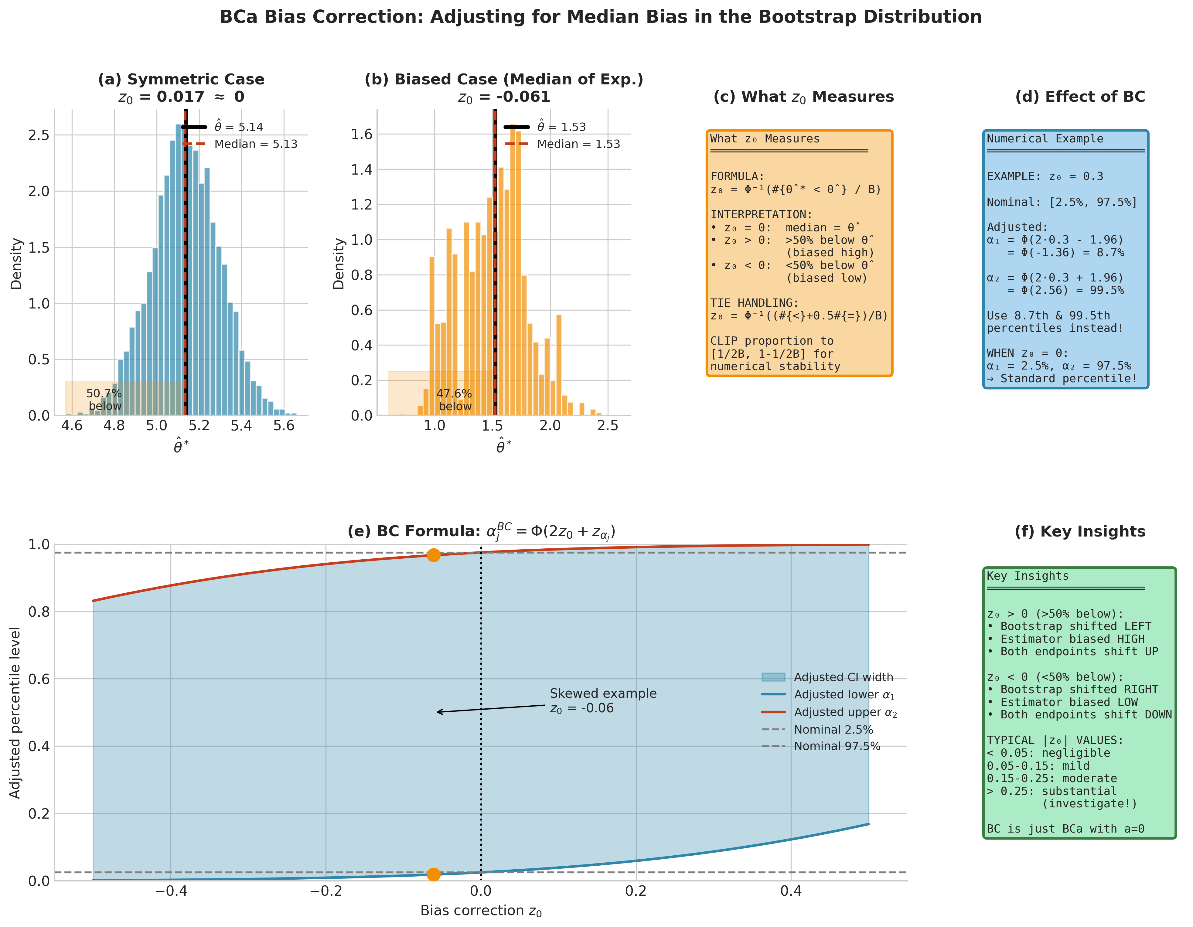
Fig. 159 Figure 4.7.4: The bias-correction constant \(z_0\). (a) Symmetric bootstrap distribution: \(z_0 \approx 0\) indicates no median bias. (b) Skewed bootstrap distribution: \(z_0 < 0\) (or \(> 0\)) indicates the bootstrap median differs from \(\hat{\theta}\). (c) Formula and interpretation of \(z_0\). (d) Numerical example showing how \(z_0\) adjusts percentile levels. (e) The BC formula visualization showing how adjusted levels vary with \(z_0\). (f) Key insights about the direction and magnitude of corrections.
Bias-Corrected and Accelerated (BCa) Intervals
The BCa interval, introduced by Efron (1987), is widely regarded as the best general-purpose bootstrap confidence interval. It achieves second-order accuracy, is transformation-invariant, and automatically adapts to bias and skewness without requiring explicit studentization. The “cost” is computing an additional acceleration parameter from the jackknife.
Theoretical Foundation
The BCa method can be motivated as a higher order calibration of bootstrap percentiles. Under standard regularity conditions for smooth functionals, there exists an unknown monotone transformation \(\phi\) such that the transformed estimator \(\hat{\phi} = \phi(\hat{\theta})\) is approximately normal and admits an Edgeworth type expansion. In that expansion, two effects dominate the coverage error of naive percentile procedures:
Median bias of \(\hat{\theta}\) relative to the bootstrap distribution.
Skewness and non constant curvature effects associated with the statistic’s influence function.
BCa incorporates these effects through two constants:
The bias correction \(z_0\), which measures median bias in standard normal units.
The acceleration \(a\), which captures the leading skewness or curvature contribution and is estimated from jackknife leave one out values.
A key feature is that BCa is invariant under monotone reparameterizations: if the parameter is replaced by \(\psi(\theta)\) for a monotone \(\psi\), the BCa construction transforms accordingly, so the resulting interval on the original scale is coherent without needing to know \(\phi\) explicitly.
Concretely, \(z_0\) is estimated from the bootstrap distribution by
and \(a\) is estimated from jackknife leave one out estimates \(\hat{\theta}_{(i)}\) via
These definitions align with the standard BCa derivation: \(z_0\) corrects median bias, and \(a\) adjusts for skewness and curvature effects that otherwise produce \(O(n^{-1/2})\) one sided coverage errors.
The BCa Formula
Given the bias correction constant \(z_0\) and acceleration constant \(a\), the BCa interval uses adjusted percentile levels:
for \(\alpha_j \in \{\alpha/2, 1-\alpha/2\}\). The BCa interval is:
Special cases:
When \(a = 0\): The BCa formula (124) reduces to \(\alpha_j^{BCa} = \Phi(2z_0 + z_{\alpha_j})\), which is exactly the BC interval.
When \(z_0 = 0\) and \(a = 0\): The formula gives \(\alpha_j^{BCa} = \alpha_j\), recovering the standard percentile interval.
Computing the Bias-Correction Constant \(z_0\)
The bias-correction constant, defined in (122) above, measures where \(\hat{\theta}\) falls in its bootstrap distribution:
Handling ties: When some bootstrap replicates exactly equal \(\hat{\theta}\) (common for discrete statistics or medians), the standard formula can overestimate bias. A robust adjustment assigns half of the ties to each side:
Numerical stability: If the proportion is exactly 0 or 1, \(\Phi^{-1}\) returns \(\mp\infty\). Clip the proportion to \([1/(2B), 1-1/(2B)]\) before applying \(\Phi^{-1}\):
def compute_z0(theta_star, theta_hat):
    """
    Compute BCa bias-correction constant with tie handling.

    Parameters
    ----------
    theta_star : array_like
        Bootstrap replicates.
    theta_hat : float
        Original estimate.

    Returns
    -------
    z0 : float
        Bias-correction constant.
    """
    from scipy.stats import norm

    theta_star = np.asarray(theta_star)
    B = len(theta_star)

    # Count with mid-rank adjustment for ties
    n_below = np.sum(theta_star < theta_hat)
    n_equal = np.sum(theta_star == theta_hat)
    prop = (n_below + 0.5 * n_equal) / B

    # Clip for numerical stability
    prop = np.clip(prop, 1 / (2 * B), 1 - 1 / (2 * B))

    return norm.ppf(prop)
Computing the Acceleration Constant \(a\)
The acceleration constant captures how the standard error of \(\hat{\theta}\) changes with the parameter value. It is computed from the jackknife influence values introduced in Section 4.5.
Let \(\hat{\theta}_{(-i)}\) be the statistic computed with observation \(i\) deleted, and let \(\bar{\theta}_{(\cdot)} = \frac{1}{n}\sum_{i=1}^n \hat{\theta}_{(-i)}\) be their mean. The acceleration constant, restating (123) from the theoretical foundation in computational form, is:
Interpretation: This formula is essentially the skewness of the jackknife influence values, normalized appropriately. Large \(|a|\) indicates that individual observations have asymmetric influence on the estimate, which corresponds to the standard error varying with the parameter.
Typical values: In many smooth problems the acceleration is small, with \(|a|\) frequently below 0.1 in practice, but it can be larger for heavy tailed data, bounded parameters, or strongly influential observations. Values above roughly 0.25 typically signal substantial acceleration effects and justify preferring BCa over BC.
Numerical guard: If all jackknife estimates are identical (denominator is zero), set \(a = 0\) and fall back to the BC interval. This can occur for statistics that are insensitive to individual observations.
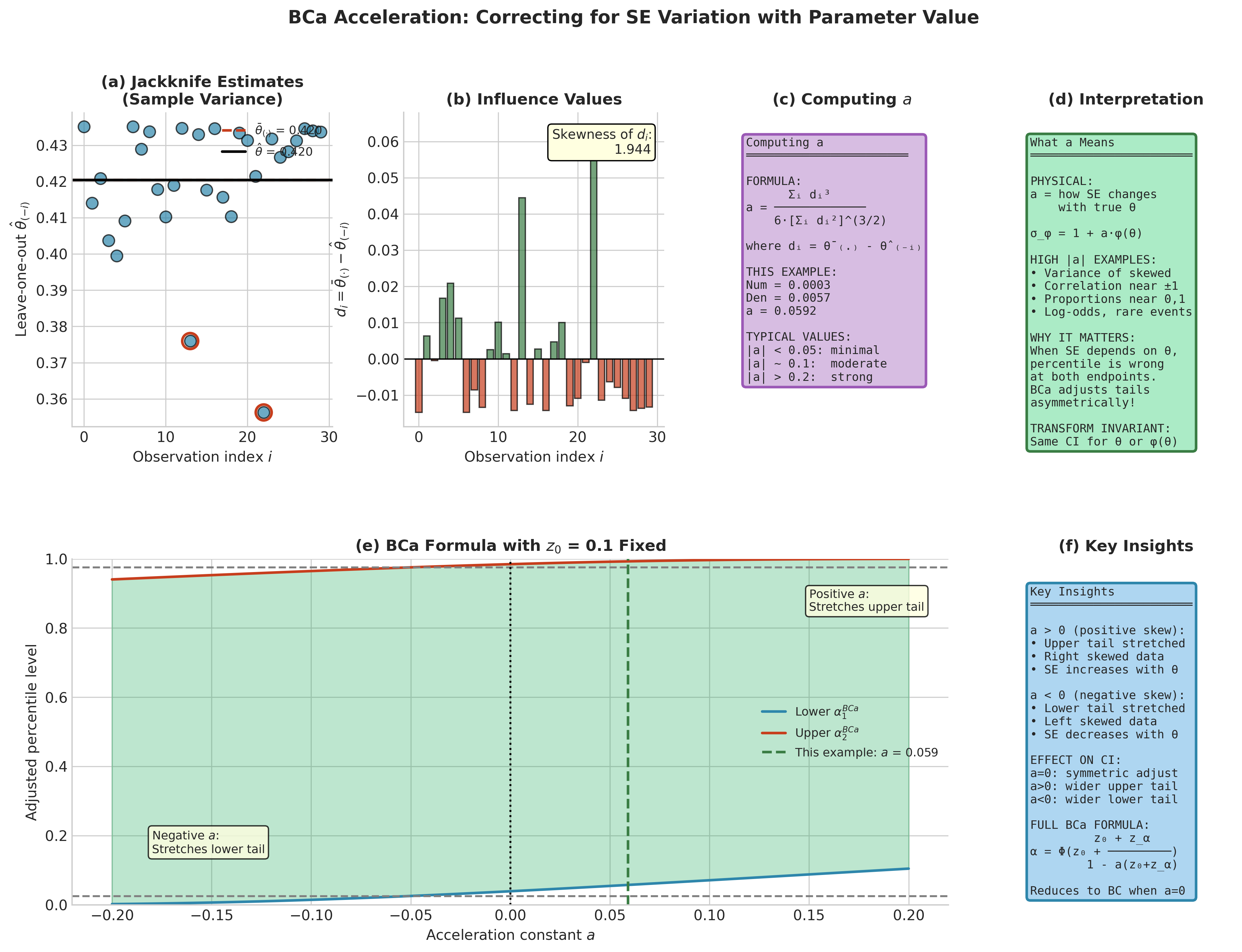
Fig. 160 Figure 4.7.5: The acceleration constant \(a\). (a) Jackknife estimates \(\hat{\theta}_{(-i)}\) for sample variance—note the influential outliers. (b) Influence values \(d_i = \bar{\theta}_{(\cdot)} - \hat{\theta}_{(-i)}\) showing skewness. (c) Formula for computing \(a\) from the skewness of influence values. (d) Interpretation: \(a\) captures how SE varies with the parameter value. (e) The full BCa formula showing how both \(z_0\) and \(a\) jointly adjust percentile levels. (f) Key insights about positive vs negative \(a\) and its effect on interval tails.
def compute_acceleration(data, statistic):
    """
    Compute BCa acceleration constant via jackknife.

    Parameters
    ----------
    data : array_like
        Original data.
    statistic : callable
        Function computing the statistic.

    Returns
    -------
    a : float
        Acceleration constant.
    theta_jack : ndarray
        Jackknife estimates (useful for diagnostics).
    """
    data = np.asarray(data)
    n = len(data)

    # Compute leave-one-out estimates
    theta_jack = np.empty(n)
    for i in range(n):
        data_minus_i = np.delete(data, i)
        theta_jack[i] = statistic(data_minus_i)

    # Compute acceleration
    theta_bar = theta_jack.mean()
    d = theta_bar - theta_jack  # Influence-like quantities

    numerator = np.sum(d**3)
    denominator = 6 * (np.sum(d**2))**1.5

    if denominator < 1e-10:
        # Degenerate case: all jackknife estimates equal
        return 0.0, theta_jack

    a = numerator / denominator
    return a, theta_jack
Transformation Invariance
A crucial property of BCa intervals is transformation invariance: if \(\psi = m(\theta)\) for a monotone function \(m\), then the BCa interval for \(\psi\) is exactly \(m\) applied to the BCa interval for \(\theta\).
Why this matters: Consider estimating a variance \(\sigma^2\). Should we compute the interval on the variance scale or the standard deviation scale? For percentile intervals (which are also transformation-invariant), we get the same answer either way. But for basic intervals or normal approximations, the choice of scale affects the result. BCa preserves this desirable invariance while achieving better coverage.
Proof sketch: The BCa adjustment formula depends on \(z_0\) and \(a\), both computed from the data without reference to the parameterization. Under a monotone transformation \(m\), the proportion of bootstrap replicates below the original estimate is preserved (since \(m(\hat{\theta}^*) < m(\hat{\theta})\) iff \(\hat{\theta}^* < \hat{\theta}\) for increasing \(m\)), so \(z_0\) is unchanged. The acceleration \(a\) transforms consistently because influence values transform linearly for smooth \(m\). Therefore, the adjusted percentile levels \(\alpha_j^{BCa}\) are invariant, and the interval endpoints transform correctly.
Complete BCa Implementation
import numpy as np
from scipy import stats

def bca_bootstrap_ci(data, statistic, alpha=0.05, B=10000, seed=None):
    """
    Compute BCa (bias-corrected and accelerated) bootstrap confidence interval.

    Parameters
    ----------
    data : array_like
        Original data.
    statistic : callable
        Function computing the statistic: statistic(data) -> float.
    alpha : float
        Significance level (default 0.05 for 95% CI).
    B : int
        Number of bootstrap replicates.
    seed : int, optional
        Random seed for reproducibility.

    Returns
    -------
    ci : tuple
        (lower, upper) confidence bounds.
    theta_hat : float
        Original point estimate.
    info : dict
        Diagnostic information including z0, a, adjusted alpha levels.
    """
    rng = np.random.default_rng(seed)
    data = np.asarray(data)
    n = len(data)

    # Original estimate
    theta_hat = statistic(data)

    # Bootstrap distribution
    theta_star = np.empty(B)
    for b in range(B):
        idx = rng.integers(0, n, size=n)
        theta_star[b] = statistic(data[idx])

    # Bias correction constant z0
    n_below = np.sum(theta_star < theta_hat)
    n_equal = np.sum(theta_star == theta_hat)
    prop = (n_below + 0.5 * n_equal) / B
    prop = np.clip(prop, 1 / (2 * B), 1 - 1 / (2 * B))
    z0 = stats.norm.ppf(prop)

    # Acceleration constant via jackknife
    theta_jack = np.empty(n)
    for i in range(n):
        data_minus_i = np.delete(data, i)
        theta_jack[i] = statistic(data_minus_i)

    theta_bar = theta_jack.mean()
    d = theta_bar - theta_jack

    numerator = np.sum(d**3)
    denominator = 6 * (np.sum(d**2))**1.5

    if denominator > 1e-10:
        a = numerator / denominator
    else:
        a = 0.0

    # Adjusted percentile levels
    z_alpha_lo = stats.norm.ppf(alpha / 2)
    z_alpha_hi = stats.norm.ppf(1 - alpha / 2)

    def adjusted_alpha(z_alpha):
        """Compute BCa-adjusted percentile level."""
        numer = z0 + z_alpha
        denom = 1 - a * (z0 + z_alpha)
        if abs(denom) < 1e-10:
            # Extreme case: return edge of [0, 1]
            return 0.0 if numer < 0 else 1.0
        return stats.norm.cdf(z0 + numer / denom)

    alpha1 = adjusted_alpha(z_alpha_lo)
    alpha2 = adjusted_alpha(z_alpha_hi)

    # Ensure valid probability range
    alpha1 = np.clip(alpha1, 1 / B, 1 - 1 / B)
    alpha2 = np.clip(alpha2, 1 / B, 1 - 1 / B)
    if alpha1 >= alpha2:
     alpha1, alpha2 = alpha/2, 1-alpha/2
     bca_warning = "Adjusted levels crossed; fell back to percentile."
    else:
     bca_warning = None

    # BCa interval
    ci_lower = np.quantile(theta_star, alpha1)
    ci_upper = np.quantile(theta_star, alpha2)

    info = {
        'z0': z0,
        'a': a,
        'alpha1': alpha1,
        'alpha2': alpha2,
        'theta_star': theta_star,
        'theta_jack': theta_jack,
        'se_boot': np.std(theta_star, ddof=1),
        'bias_boot': theta_star.mean() - theta_hat,
        'bca_warning': bca_warning
    }

    return (ci_lower, ci_upper), theta_hat, info
Example 💡 BCa Interval for Median of Skewed Data
Given: A sample of \(n = 60\) observations from a log-normal distribution (positively skewed).
Find: A 95% confidence interval for the population median.
Challenge: The bootstrap distribution of the sample median is skewed, and the median is a non-smooth statistic.
Python implementation:
import numpy as np
from scipy import stats

# Generate skewed data
rng = np.random.default_rng(42)
n = 60
# Log-normal with median = exp(0) = 1
data = np.exp(rng.normal(0, 1, size=n))

true_median = 1.0  # exp(0) for lognormal(0, 1)

def sample_median(x):
    return np.median(x)

# BCa interval
ci_bca, med_hat, info = bca_bootstrap_ci(
    data, sample_median, alpha=0.05, B=10000, seed=123
)

# Percentile interval for comparison
theta_star = info['theta_star']
ci_perc = (np.quantile(theta_star, 0.025),
           np.quantile(theta_star, 0.975))

# Basic interval
q_lo = np.quantile(theta_star, 0.025)
q_hi = np.quantile(theta_star, 0.975)
ci_basic = (2 * med_hat - q_hi, 2 * med_hat - q_lo)

print(f"Sample median: {med_hat:.4f}")
print(f"True median:   {true_median:.4f}")
print(f"z0 = {info['z0']:.4f}, a = {info['a']:.4f}")
print(f"Adjusted levels: [{info['alpha1']:.4f}, {info['alpha2']:.4f}]")
print(f"\n95% Confidence Intervals:")
print(f"  Percentile: [{ci_perc[0]:.4f}, {ci_perc[1]:.4f}]")
print(f"  Basic:      [{ci_basic[0]:.4f}, {ci_basic[1]:.4f}]")
print(f"  BCa:        [{ci_bca[0]:.4f}, {ci_bca[1]:.4f}]")
Typical output:
Sample median: 1.1301
True median:   1.0000
z0 = -0.0084, a = 0.0000
Adjusted levels: [0.0240, 0.9740]

95% Confidence Intervals:
  Percentile: [0.8312, 1.4459]
  Basic:      [0.8142, 1.4289]
  BCa:        [0.8312, 1.4459]
Interpretation: For this sample both corrections are essentially zero. The small negative \(z_0 = -0.0084\) says the bootstrap distribution is nearly median-unbiased, and the acceleration is exactly zero: with an even sample size the leave-one-out medians take just two values placed symmetrically about their mean, so the jackknife skewness vanishes. The adjusted percentile levels [2.40%, 97.40%] barely move from the nominal [2.5%, 97.5%], and the BCa interval coincides with the percentile interval to four decimals. This illustrates that BCa is adaptive—when no correction is needed, it reduces to the percentile interval—but also that the jackknife acceleration estimate can be degenerate for non-smooth statistics like the median.
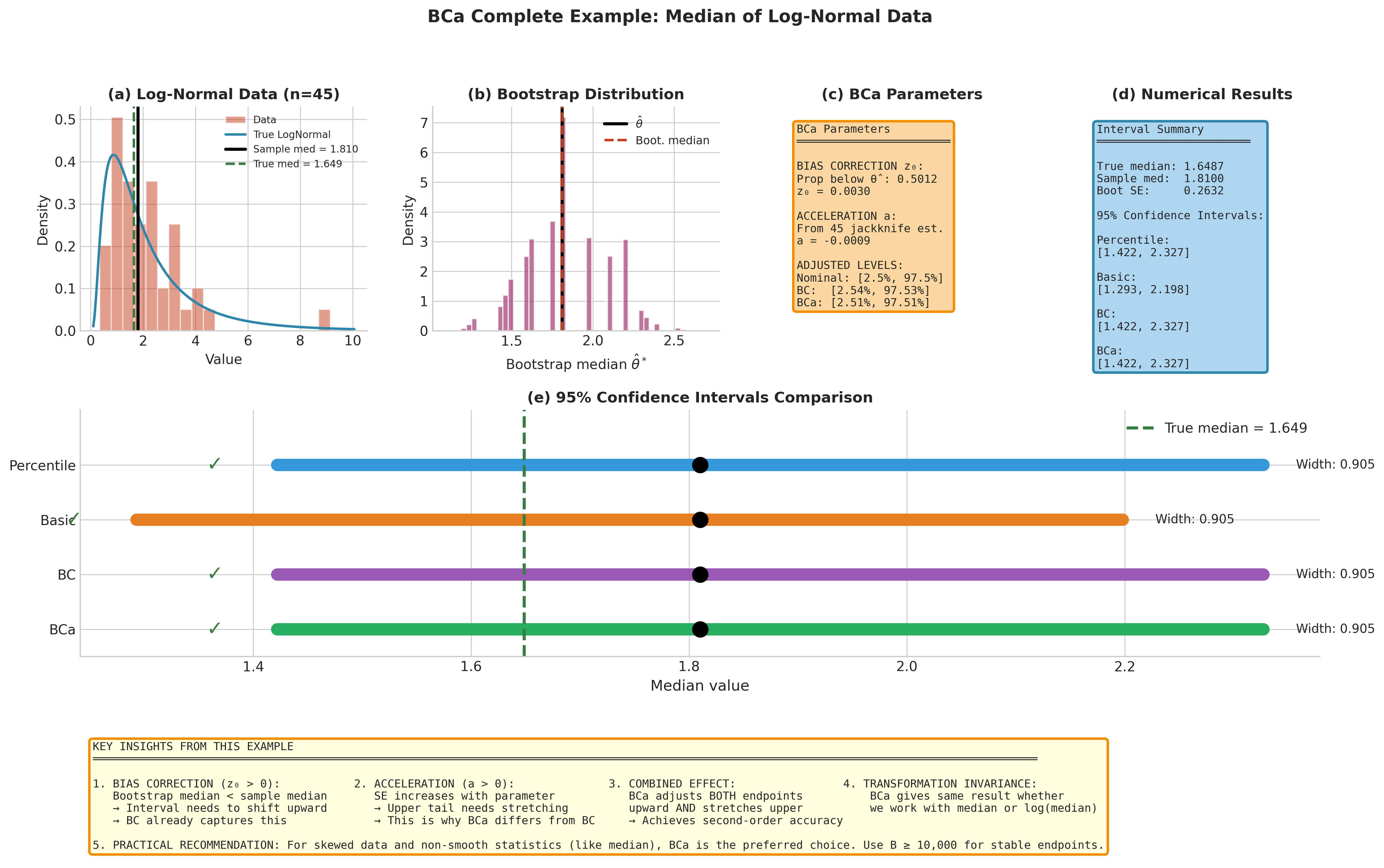
Fig. 161 Figure 4.7.6: Complete BCa example for median of log-normal data. (a) The skewed log-normal data with true and sample medians marked. (b) Bootstrap distribution of the sample median. (c) Computed BCa parameters \(z_0\) and \(a\) with adjusted percentile levels. (d) Numerical results for all confidence interval methods. (e) Visual comparison of the four interval methods showing which capture the true median. Key insights at the bottom explain how bias correction and acceleration work together.
The log-normal median above is a case where BCa makes no correction. The law-school correlation is the opposite extreme—a bounded parameter on a small, skewed sample, where BCa matters most. It is also the dataset Efron (1987) used to introduce the method.
Example 💡 BCa Interval for the Law-School Correlation
Given: The Efron–Tibshirani law-school data (\(n = 15\) schools, LSAT vs GPA), with sample correlation \(\hat{r} = 0.776\). In Section 4.3 the percentile interval was [0.456, 0.962], while the basic and normal intervals ran past the boundary \(\rho = 1\).
Find: The BCa interval, and how its bias-correction and acceleration constants reshape the percentile interval.
Python implementation: Because the correlation requires resampling (LSAT, GPA) pairs together, we compute the BCa constants directly rather than through the one-sample bca_bootstrap_ci helper above:
import numpy as np
import pandas as pd
from scipy import stats

# Efron-Tibshirani law-school data (n = 15): the classic BCa motivating example
url = "https://pqyjaywwccbnqpwgeiuv.supabase.co/storage/v1/object/public/STAT%20418%20Images/Data/Chapter4/law_school.csv"
df = pd.read_csv(url)
lsat = df["LSAT"].to_numpy(float)
gpa = df["GPA"].to_numpy(float)
n = lsat.size
r_hat = np.corrcoef(lsat, gpa)[0, 1]

# Pairs bootstrap of the correlation
B = 10_000
rng = np.random.default_rng(42)
r_star = np.empty(B)
for b in range(B):
    idx = rng.integers(0, n, size=n)
    r_star[b] = np.corrcoef(lsat[idx], gpa[idx])[0, 1]

# Bias-correction z0: normal quantile of the share of replicates below r_hat
z0 = stats.norm.ppf(np.mean(r_star < r_hat))

# Acceleration a: from the jackknife (leave-one-out) influence values
jack = np.array([np.corrcoef(np.delete(lsat, i), np.delete(gpa, i))[0, 1]
                 for i in range(n)])
jbar = jack.mean()
a = np.sum((jbar - jack) ** 3) / (6.0 * np.sum((jbar - jack) ** 2) ** 1.5)

# BCa-adjusted percentile levels
def bca_endpoint(p):
    zp = stats.norm.ppf(p)
    adj = z0 + (z0 + zp) / (1 - a * (z0 + zp))
    return np.quantile(r_star, stats.norm.cdf(adj))

ci_perc = np.quantile(r_star, [0.025, 0.975])
ci_bca = (bca_endpoint(0.025), bca_endpoint(0.975))

print(f"r_hat = {r_hat:.4f}")
print(f"z0 = {z0:.4f},  a = {a:.4f}")
print(f"Percentile CI: [{ci_perc[0]:.3f}, {ci_perc[1]:.3f}]")
print(f"BCa CI:        [{ci_bca[0]:.3f}, {ci_bca[1]:.3f}]")
Output:
r_hat = 0.7764
z0 = -0.1055,  a = -0.0757
Percentile CI: [0.456, 0.962]
BCa CI:        [0.317, 0.943]
Interpretation: Both constants are now firmly non-zero. The bias correction \(z_0 = -0.106\) reflects that only about 46% of bootstrap replicates fall below \(\hat{r}\)—the distribution is left-skewed, piled up near the boundary—and the acceleration \(a = -0.076\) captures the skewness of the jackknife influence values. Together they pull the interval downward to [0.317, 0.943]: the lower limit drops from 0.456 (percentile) all the way to 0.317. That is a substantial correction the first-order percentile interval misses. BCa thus threads the needle that the basic and normal intervals could not—it stays inside \([-1, 1]\) like the percentile interval, yet, unlike percentile, it accounts for the bias and skewness that small-sample correlations exhibit. (The matching skewness and Q–Q diagnostics for this bootstrap appear in Section 4.3, Figure 4.3.6.)
When BCa Fails
The law-school case succeeded because BCa improved on every alternative even at \(n = 15\)—but that relative win does not make BCa universally safe. Its absolute coverage can still degrade in several regimes:
Non-smooth statistics: The jackknife-based acceleration formula assumes smooth dependence on individual observations. For highly non-smooth statistics (sample mode, range, extreme quantiles), the jackknife estimates \(\hat{\theta}_{(-i)}\) may be unstable, leading to unreliable \(a\).
Very small samples: When \(n < 15\), the jackknife provides only a coarse approximation to influence, and BCa coverage can be substantially below nominal. For \(n < 10\), consider parametric methods or exact approaches.
Multimodal bootstrap distributions: BCa assumes a unimodal, roughly symmetric underlying structure. Multimodality indicates a fundamental problem that no simple adjustment can fix.
Boundary effects: For parameters near natural boundaries (proportions near 0 or 1, variances near 0, correlations near \(\pm 1\)), the BCa formula may produce adjusted levels \(\alpha_j^{BCa}\) outside \((0, 1)\), requiring truncation.
Choosing B and Assessing Monte Carlo Error
Every bootstrap computation involves Monte Carlo error—the additional randomness from using finitely many bootstrap replicates \(B\). This error is distinct from the statistical uncertainty we’re trying to quantify (which depends on the sample size \(n\)) and is under our control. Choosing \(B\) appropriately and understanding Monte Carlo error are essential for responsible bootstrap inference.
Two Sources of Uncertainty
Consider a bootstrap standard error estimate \(\widehat{\text{SE}}_{\text{boot}} = \text{SD}(\hat{\theta}^*)\). This estimate has two sources of variability:
Statistical uncertainty: The bootstrap SE estimates the true standard error \(\text{SE}_F(\hat{\theta})\), which depends on the unknown distribution \(F\). Even with \(B = \infty\), our estimate reflects only what the sample tells us about \(F\).
Monte Carlo uncertainty: With finite \(B\), we approximate the bootstrap distribution with a Monte Carlo sample. This adds noise that disappears as \(B \to \infty\) but contributes to estimation error for finite \(B\).
The goal: Choose \(B\) large enough that Monte Carlo error is negligible relative to statistical uncertainty. We cannot eliminate statistical uncertainty, but we can make Monte Carlo error as small as computational resources allow.
Monte Carlo Error for Bootstrap SE
Under mild conditions, the bootstrap replicates \(\hat{\theta}^*_1, \ldots, \hat{\theta}^*_B\) are approximately iid draws from the bootstrap distribution. The sample standard deviation \(\widehat{\text{SE}}_{\text{boot}} = \text{SD}(\hat{\theta}^*)\) estimates the population standard deviation of this distribution.
For the standard deviation of iid random variables, the Monte Carlo standard error is approximately:
This gives the coefficient of variation of the bootstrap SE estimate:
Practical implications:
Replicates \(B\) |
CV of SE estimate |
Interpretation |
|---|---|---|
200 |
5.0% |
Rough approximation |
500 |
3.2% |
Reasonable for exploration |
1,000 |
2.2% |
Standard practice |
2,000 |
1.6% |
Good precision |
10,000 |
0.7% |
High precision |
For most applications, \(B = 1{,}000\text{--}2{,}000\) provides bootstrap SE estimates with acceptable Monte Carlo error.
Monte Carlo Error for Quantile Endpoints
Confidence interval endpoints require estimating quantiles of the bootstrap distribution, and quantile estimation has different Monte Carlo error characteristics than mean or SD estimation.
For the \(\alpha\)-quantile \(q_\alpha\), the Monte Carlo variance is approximately:
where \(f(q_\alpha)\) is the probability density of the bootstrap distribution at the quantile. The Monte Carlo SE is:
Key observations:
Tail quantiles are harder: For \(\alpha = 0.025\) (the 2.5th percentile), \(\alpha(1-\alpha) = 0.024\). For \(\alpha = 0.5\) (the median), \(\alpha(1-\alpha) = 0.25\). Tail quantiles have smaller numerators.
Density matters: Tail quantiles typically occur where the density \(f(q_\alpha)\) is lower, which increases MC variance. The net effect often makes tail quantile estimation harder than it might seem from \(\alpha(1-\alpha)\) alone.
More :math:`B` needed for CIs: Because CI endpoints are tail quantiles with potentially low density, they require substantially more \(B\) than SE estimation.
Estimating the Density at Quantiles
To assess Monte Carlo error for CI endpoints, we need to estimate \(f(q_\alpha)\). Two approaches:
Spacing method: Estimate the density using nearby quantiles:
for small \(\delta\) (e.g., \(\delta = 0.01\)). This uses the fact that \(P(q_{\alpha-\delta} < X < q_{\alpha+\delta}) \approx 2\delta\).
Kernel density estimation: Apply a KDE to the bootstrap replicates and evaluate at the empirical quantile.
def quantile_mc_error(theta_star, alpha, delta=0.01):
    """
    Estimate Monte Carlo standard error for a quantile estimate.

    Parameters
    ----------
    theta_star : array_like
        Bootstrap replicates.
    alpha : float
        Quantile level (e.g., 0.025 for 2.5th percentile).
    delta : float
        Half-width for density estimation.

    Returns
    -------
    se_mc : float
        Estimated MC standard error.
    f_hat : float
        Estimated density at the quantile.
    """
    B = len(theta_star)

    # Quantile estimate
    q_alpha = np.quantile(theta_star, alpha)

    # Density estimate via spacing
    alpha_lo = max(0.001, alpha - delta)
    alpha_hi = min(0.999, alpha + delta)
    q_lo = np.quantile(theta_star, alpha_lo)
    q_hi = np.quantile(theta_star, alpha_hi)

    if q_hi > q_lo:
        f_hat = (alpha_hi - alpha_lo) / (q_hi - q_lo)
    else:
        f_hat = np.inf  # Degenerate case

    # MC standard error
    se_mc = np.sqrt(alpha * (1 - alpha)) / (np.sqrt(B) * f_hat)

    return se_mc, f_hat
Practical Recommendations for Choosing B
Based on the analysis above, here are guidelines for choosing \(B\):
Task |
Recommended \(B\) |
Rationale |
|---|---|---|
Bootstrap SE only |
1,000–2,000 |
CV < 2.5% is usually adequate |
Percentile CI (95%) |
5,000–10,000 |
Tail quantiles need more precision |
BCa CI (95%) |
10,000–15,000 |
Adjusted levels may be in tails |
Bootstrap hypothesis test |
10,000–20,000 |
p-value precision matters |
Publication quality |
10,000+ |
Report stability checks |
Additional considerations:
Computation time: If each bootstrap replicate is fast (simple statistics), use larger \(B\). If expensive (complex models), balance precision against time.
Jackknife cost: BCa requires \(n\) jackknife evaluations in addition to \(B\) bootstrap evaluations. For expensive statistics with large \(n\), this may dominate.
Parallel computing: Bootstrap replicates are embarrassingly parallel. With modern hardware, \(B = 10{,}000\) is routine for most applications.
Adaptive and Batch-Based Stopping Rules
Rather than fixing \(B\) in advance, we can run bootstrap in batches and stop when estimates stabilize.
Batch-based stability check:
Run bootstrap in batches of size \(B_{\text{batch}}\) (e.g., 1,000).
After each batch, compute cumulative CI endpoints.
Stop when the change in endpoints from the previous batch is below a threshold.
def adaptive_bca_ci(data, statistic, alpha=0.05, B_batch=1000,
                     max_batches=20, tol=0.01, seed=None):
    """
    BCa CI with adaptive stopping based on endpoint stability.

    Parameters
    ----------
    data : array_like
        Original data.
    statistic : callable
        Function computing the statistic.
    alpha : float
        Significance level.
    B_batch : int
        Batch size for bootstrap replicates.
    max_batches : int
        Maximum number of batches.
    tol : float
        Relative tolerance for stopping (as fraction of SE).
    seed : int, optional
        Random seed.

    Returns
    -------
    ci : tuple
        Final (lower, upper) CI.
    info : dict
        Convergence information.
    """
    rng = np.random.default_rng(seed)
    data = np.asarray(data)
    n = len(data)

    theta_hat = statistic(data)

    # Pre-compute jackknife for acceleration (doesn't change)
    theta_jack = np.empty(n)
    for i in range(n):
        theta_jack[i] = statistic(np.delete(data, i))

    theta_bar = theta_jack.mean()
    d = theta_bar - theta_jack
    num = np.sum(d**3)
    den = 6 * (np.sum(d**2))**1.5
    a = num / den if den > 1e-10 else 0.0

    # Accumulate bootstrap replicates
    theta_star_all = []
    ci_history = []
    prev_ci = None

    for batch in range(max_batches):
        # Generate batch of bootstrap replicates
        theta_star_batch = np.empty(B_batch)
        for b in range(B_batch):
            idx = rng.integers(0, n, size=n)
            theta_star_batch[b] = statistic(data[idx])

        theta_star_all.extend(theta_star_batch)
        theta_star = np.array(theta_star_all)
        B_current = len(theta_star)

        # Compute BCa CI with current replicates
        prop = (np.sum(theta_star < theta_hat) +
                0.5 * np.sum(theta_star == theta_hat)) / B_current
        prop = np.clip(prop, 1 / (2 * B_current), 1 - 1 / (2 * B_current))
        z0 = stats.norm.ppf(prop)

        z_lo = stats.norm.ppf(alpha / 2)
        z_hi = stats.norm.ppf(1 - alpha / 2)

        def adj_alpha(z):
            numer = z0 + z
            denom = 1 - a * (z0 + z)
            if abs(denom) < 1e-10:
                return 0.0 if numer < 0 else 1.0
            return stats.norm.cdf(z0 + numer / denom)

        alpha1 = np.clip(adj_alpha(z_lo), 1/B_current, 1-1/B_current)
        alpha2 = np.clip(adj_alpha(z_hi), 1/B_current, 1-1/B_current)

        ci = (np.quantile(theta_star, alpha1),
              np.quantile(theta_star, alpha2))
        ci_history.append(ci)

        # Check convergence
        if prev_ci is not None:
            se_boot = np.std(theta_star, ddof=1)
            change = max(abs(ci[0] - prev_ci[0]), abs(ci[1] - prev_ci[1]))
            rel_change = change / se_boot if se_boot > 0 else 0

            if rel_change < tol:
                break

        prev_ci = ci

    info = {
        'B_total': len(theta_star_all),
        'n_batches': batch + 1,
        'converged': (batch + 1) < max_batches,
        'ci_history': ci_history,
        'z0': z0,
        'a': a
    }

    return ci, info
Reporting Monte Carlo Error
For publication-quality results, report Monte Carlo error alongside bootstrap estimates:
# After computing BCa CI
ci, theta_hat, info = bca_bootstrap_ci(data, statistic, B=10000, seed=42)

# Compute MC errors for endpoints
se_mc_lo, _ = quantile_mc_error(info['theta_star'], info['alpha1'])
se_mc_hi, _ = quantile_mc_error(info['theta_star'], info['alpha2'])

print(f"Point estimate: {theta_hat:.4f}")
print(f"Bootstrap SE: {info['se_boot']:.4f}")
print(f"95% BCa CI: [{ci[0]:.4f}, {ci[1]:.4f}]")
print(f"MC SE of endpoints: ({se_mc_lo:.4f}, {se_mc_hi:.4f})")
Diagnostics for Advanced Bootstrap Methods
Before reporting any bootstrap confidence interval, examine the bootstrap distribution and method-specific quantities to ensure the results are trustworthy. This section consolidates diagnostic approaches for all the methods covered.
Visual Diagnostics
For all methods:
Histogram of \(\hat{\theta}^*\) with vertical lines marking \(\hat{\theta}\) and CI endpoints
Normal Q-Q plot of \(\hat{\theta}^*\) to assess departure from normality
Endpoint stability plot: CI bounds versus \(B\) (run in batches)
For studentized bootstrap additionally:
Histogram of \(t^*\) compared with \(N(0,1)\) or \(t_{n-1}\)
Check for extreme \(t^*\) values (indicate \(\hat{\sigma}^* \approx 0\))
For BCa additionally:
Jackknife influence plot: \(\hat{\theta}_{(-i)}\) versus \(i\) to identify influential observations
Verify adjusted levels \(\alpha_1^{BCa}, \alpha_2^{BCa}\) are not extreme
def comprehensive_bootstrap_diagnostics(data, statistic, ci_method='bca',
                                    alpha=0.05, B=10000, seed=None,
                                    batch_size=500, n_batches=10):
    """
    Generate comprehensive diagnostics for bootstrap CI.

    Parameters
    ----------
    data : array_like
        Original data.
    statistic : callable
        Function computing the statistic.
    ci_method : str
        'percentile', 'basic', or 'bca'.
    alpha : float
        Significance level.
    B : int
        Number of bootstrap replicates.
    seed : int
        Random seed.
    batch_size : int
        Size of each independent bootstrap batch used for endpoint stability.
    n_batches : int
        Number of batches to show in the endpoint stability plot.

    Returns
    -------
    fig : matplotlib.figure.Figure
        Diagnostic plots.
    diagnostics : dict
        Quantitative diagnostic summaries.
    """
    import numpy as np
    import matplotlib.pyplot as plt
    from scipy import stats

    rng = np.random.default_rng(seed)
    data = np.asarray(data)
    n = len(data)

    theta_hat = statistic(data)

    # ---------------------------------------------------------------------
    # Bootstrap distribution (single run of size B)
    # ---------------------------------------------------------------------
    theta_star = np.empty(B)
    for b in range(B):
        idx = rng.integers(0, n, size=n)
        theta_star[b] = statistic(data[idx])

    # ---------------------------------------------------------------------
    # Jackknife for BCa and diagnostics
    # ---------------------------------------------------------------------
    theta_jack = np.empty(n)
    for i in range(n):
        theta_jack[i] = statistic(np.delete(data, i))

    # Basic summaries
    se_boot = np.std(theta_star, ddof=1)
    bias_boot = theta_star.mean() - theta_hat
    skewness = stats.skew(theta_star, bias=False)
    kurtosis = stats.kurtosis(theta_star, fisher=True, bias=False)

    # BCa parameters (use a robust tie strategy; exact float ties are rare)
    prop = np.mean(theta_star < theta_hat)
    prop = np.clip(prop, 1/(2*B), 1 - 1/(2*B))
    z0 = stats.norm.ppf(prop)

    theta_bar = theta_jack.mean()
    d = theta_bar - theta_jack
    denom = np.sum(d**2)
    a = np.sum(d**3) / (6 * denom**1.5) if denom > 1e-14 else 0.0

    # ---------------------------------------------------------------------
    # Helper: compute CI from an already-generated theta_star vector
    # ---------------------------------------------------------------------
    def _ci_from_theta_star(theta_star_local, method):
        theta_star_local = np.asarray(theta_star_local)
        if method == 'percentile':
            return (np.quantile(theta_star_local, alpha/2),
                    np.quantile(theta_star_local, 1 - alpha/2))

        if method == 'basic':
            q_lo = np.quantile(theta_star_local, alpha/2)
            q_hi = np.quantile(theta_star_local, 1 - alpha/2)
            return (2 * theta_hat - q_hi, 2 * theta_hat - q_lo)

        if method == 'bca':
            z_lo = stats.norm.ppf(alpha/2)
            z_hi = stats.norm.ppf(1 - alpha/2)

            def adj(z):
                num = z0 + z
                den = 1 - a * (z0 + z)
                if abs(den) < 1e-14:
                    return 0.0 if num < 0 else 1.0
                return stats.norm.cdf(z0 + num / den)

            alpha1 = np.clip(adj(z_lo), 1 / len(theta_star_local), 1 - 1 / len(theta_star_local))
            alpha2 = np.clip(adj(z_hi), 1 / len(theta_star_local), 1 - 1 / len(theta_star_local))

            # Guard against crossing adjusted levels (rare but possible)
            if alpha1 >= alpha2:
                # fall back to percentile on the same theta_star_local
                return (np.quantile(theta_star_local, alpha/2),
                        np.quantile(theta_star_local, 1 - alpha/2))

            return (np.quantile(theta_star_local, alpha1),
                    np.quantile(theta_star_local, alpha2))

        raise ValueError(f"Unknown method: {method}")

    # Compute CI based on requested method (using the full theta_star)
    ci = _ci_from_theta_star(theta_star, ci_method)

    # ---------------------------------------------------------------------
    # Create diagnostic plots
    # ---------------------------------------------------------------------
    fig, axes = plt.subplots(2, 3, figsize=(14, 9))

    # 1. Histogram with CI
    axes[0, 0].hist(theta_star, bins=50, density=True, alpha=0.7,
                    edgecolor='white')
    axes[0, 0].axvline(theta_hat, linewidth=2,
                    label=f'$\\hat{{\\theta}}$ = {theta_hat:.3f}')
    axes[0, 0].axvline(ci[0], linestyle='--', linewidth=2,
                    label=f'CI: [{ci[0]:.3f}, {ci[1]:.3f}]')
    axes[0, 0].axvline(ci[1], linestyle='--', linewidth=2)
    axes[0, 0].set_xlabel('$\\hat{\\theta}^*$')
    axes[0, 0].set_ylabel('Density')
    axes[0, 0].set_title('Bootstrap Distribution')
    axes[0, 0].legend(fontsize=9)

    # 2. Normal Q-Q plot
    stats.probplot(theta_star, dist="norm", plot=axes[0, 1])
    axes[0, 1].set_title('Normal Q-Q Plot')

    # 3. Jackknife influence
    axes[0, 2].scatter(range(n), theta_jack, alpha=0.6, s=30)
    axes[0, 2].axhline(theta_bar, linestyle='--',
                    label=f'Mean = {theta_bar:.3f}')
    axes[0, 2].set_xlabel('Observation Index')
    axes[0, 2].set_ylabel('$\\hat{\\theta}_{(-i)}$')
    axes[0, 2].set_title('Jackknife Leave One Out Estimates')
    axes[0, 2].legend()

    # 4. Bias ratio visualization
    bias_ratio = abs(bias_boot) / se_boot if se_boot > 0 else np.nan
    axes[1, 0].barh(['Bias Ratio'], [bias_ratio])
    axes[1, 0].axvline(0.25, linestyle='--', label='Warning (0.25)')
    axes[1, 0].axvline(0.5, linestyle='--', label='Concern (0.5)')
    axes[1, 0].set_xlim(0, max(1, (bias_ratio if np.isfinite(bias_ratio) else 0) * 1.2))
    axes[1, 0].set_xlabel('|Bias| / SE')
    axes[1, 0].set_title(f'Bias Ratio = {bias_ratio:.3f}' if np.isfinite(bias_ratio) else 'Bias Ratio')
    axes[1, 0].legend()

    # 5. Endpoint stability using independent batches
    #    This shows how endpoints change as you aggregate *independent* bootstrap batches.
    #    We generate n_batches batches of size batch_size, compute CI after k batches.
    total_for_stability = batch_size * n_batches
    theta_star_batches = np.empty(total_for_stability)

    # Use a new RNG stream to keep the main theta_star fixed given the seed
    rng_stab = np.random.default_rng(None if seed is None else seed + 1)

    for b in range(total_for_stability):
        idx = rng_stab.integers(0, n, size=n)
        theta_star_batches[b] = statistic(data[idx])

    B_values = np.arange(batch_size, total_for_stability + 1, batch_size)
    ci_lo_hist = []
    ci_hi_hist = []
    for b in B_values:
        ci_b = _ci_from_theta_star(theta_star_batches[:b], ci_method)
        ci_lo_hist.append(ci_b[0])
        ci_hi_hist.append(ci_b[1])

    axes[1, 1].plot(B_values, ci_lo_hist, label='Lower')
    axes[1, 1].plot(B_values, ci_hi_hist, label='Upper')
    axes[1, 1].set_xlabel('Total replicates used (independent batches)')
    axes[1, 1].set_ylabel('CI endpoint')
    axes[1, 1].set_title(f'Endpoint Stability ({ci_method.upper()}, batch size = {batch_size})')
    axes[1, 1].legend()

    # 6. Summary statistics text
    summary_text = (
        f"Sample size n = {n}\n"
        f"Bootstrap B = {B}\n"
        f"$\\hat{{\\theta}}$ = {theta_hat:.4f}\n"
        f"Bootstrap SE = {se_boot:.4f}\n"
        f"Bootstrap Bias = {bias_boot:.4f}\n"
        f"Skewness = {skewness:.3f}\n"
        f"Kurtosis = {kurtosis:.3f}\n"
        f"$z_0$ = {z0:.4f}\n"
        f"$a$ = {a:.4f}\n"
        f"Method: {ci_method.upper()}\n"
        f"CI: [{ci[0]:.4f}, {ci[1]:.4f}]"
    )
    axes[1, 2].text(0.05, 0.5, summary_text, transform=axes[1, 2].transAxes,
                    fontsize=11, verticalalignment='center', fontfamily='monospace',
                    bbox=dict(boxstyle='round', facecolor='wheat', alpha=0.5))
    axes[1, 2].axis('off')
    axes[1, 2].set_title('Summary Statistics')

    plt.tight_layout()

    diagnostics = {
        'se_boot': se_boot,
        'bias_boot': bias_boot,
        'bias_ratio': bias_ratio,
        'skewness': skewness,
        'kurtosis': kurtosis,
        'z0': z0,
        'a': a,
        'ci': ci,
        'theta_hat': theta_hat,
        'theta_star': theta_star,
        'theta_jack': theta_jack,
        # stability series for programmatic inspection
        'stability_B_values': B_values,
        'stability_ci_lower': np.array(ci_lo_hist),
        'stability_ci_upper': np.array(ci_hi_hist),
        'stability_method': ci_method,
        'stability_batch_size': batch_size,
        'stability_n_batches': n_batches
    }

    return fig, diagnostics
Quantitative Diagnostic Thresholds
Use these thresholds to guide method selection and identify potential problems:
Diagnostic |
Threshold |
Action |
|---|---|---|
Bias ratio \(|\text{bias}|/\text{SE}\) |
< 0.25 |
Bias correction unnecessary |
0.25–0.5 |
Consider BC or BCa |
|
> 0.5 |
Use BCa; report both corrected and uncorrected |
|
Skewness \(|\gamma_1|\) |
< 0.5 |
Normal approximation may suffice |
0.5–2 |
Use BCa or studentized |
|
> 2 |
Bootstrap may be problematic; investigate |
|
\(|z_0|\) |
< 0.1 |
Minimal bias correction |
0.1–0.5 |
Moderate bias; BCa appropriate |
|
> 0.5 |
Large bias; verify data and statistic |
|
Acceleration \(|a|\) |
< 0.05 |
BC suffices (a ≈ 0) |
0.05–0.2 |
BCa provides improvement |
|
> 0.2 |
Strong acceleration; BCa essential |
|
Adjusted levels \(\alpha_j^{BCa}\) |
In (0.001, 0.999) |
Normal operation |
Near 0 or 1 |
Extreme correction; verify results |
Red Flags Requiring Further Investigation
Critical warnings (do not trust results without investigation):
Multimodal bootstrap distribution: Indicates instability, data issues, or inappropriate statistic
Many identical bootstrap estimates: Common with discrete data; consider smoothed bootstrap
Extreme :math:`t^*` values (studentized): Check for near-zero \(\hat{\sigma}^*\)
Adjusted BCa levels outside (0.01, 0.99): Very extreme correction; results may be unreliable
CI endpoints at sample extremes: Bootstrap cannot extrapolate beyond data
Moderate warnings (proceed with caution):
Bias ratio > 0.5 without clear explanation
Kurtosis > 10 (heavy tails)
Large change in endpoints when increasing \(B\)
Jackknife estimates show strong outliers
Common Pitfall ⚠️
Ignoring diagnostics and reporting only the CI
A bootstrap CI is not a magic number. The bootstrap distribution contains rich information about the sampling behavior of your statistic. Always examine:
The shape of the bootstrap distribution
The bias and acceleration parameters
The stability of endpoints with respect to \(B\)
If diagnostics reveal problems, report them alongside the interval or consider alternative methods.
Method Selection Guide
With four main interval methods available (percentile, basic, studentized, BCa), choosing the right one depends on the characteristics of your statistic, the sample size, and the available computational resources.
Decision Framework
Step 1: Examine the bootstrap distribution
Run a bootstrap with \(B = 10{,}000\) and examine \(\hat{\theta}^*\):
Is it unimodal? If not, investigate before proceeding.
Is it roughly symmetric? If yes, simpler methods may suffice.
Is there notable skewness? BCa or studentized are preferred.
Step 2: Assess bias
Compute \(z_0\) and the bias ratio \(|\text{bias}|/\text{SE}\):
Bias ratio < 0.25: Percentile or basic intervals are adequate
Bias ratio > 0.25: Use BCa (or BC if acceleration is negligible)
Step 3: Consider SE availability
Reliable analytical SE formula exists: Studentized bootstrap is available and achieves best accuracy
SE requires complex estimation: BCa avoids nested computation
Step 4: Evaluate computational constraints
Expensive statistic, moderate \(n\): BCa (jackknife adds \(n\) evaluations)
Very expensive statistic: Percentile with large \(B\) may be practical compromise
Cheap statistic: Use studentized with jackknife SE, or BCa with \(B = 15{,}000+\)
Summary Comparison
Method |
Coverage Error (one-sided) |
Coverage Error (two-sided) |
Transform Invariant |
Computation |
Best For |
Limitations |
|---|---|---|---|---|---|---|
Percentile |
\(O(n^{-1/2})\) |
\(O(n^{-1})\) |
Yes |
Low |
Quick assessment; symmetric cases |
Bias drift; poor one-sided |
Basic |
\(O(n^{-1/2})\) |
\(O(n^{-1})\) |
No |
Low |
Slight asymmetry; centered output |
Not transformation invariant |
BC |
\(O(n^{-1/2})\) |
\(O(n^{-1})\) |
Yes |
Low |
Bias without acceleration |
Doesn’t correct for skewness |
BCa |
\(O(n^{-1})\) |
\(O(n^{-1})\) |
Yes |
Medium |
General-purpose default |
Non-smooth statistics |
Studentized |
\(O(n^{-1})\) |
\(O(n^{-1})\) |
No |
High |
Best theoretical accuracy |
Requires SE estimation |
Practical recommendations:
Default choice: BCa with \(B \geq 10{,}000\). It handles bias and acceleration automatically, is transformation-invariant, and works well for most statistics.
When accuracy is paramount: Studentized bootstrap, if a reliable SE formula exists or jackknife SE is stable.
For quick exploration: Percentile with \(B = 2{,}000\text{--}5{,}000\).
For non-smooth statistics (median, quantiles): Percentile or smoothed bootstrap; BCa’s jackknife may be unreliable.
Bringing It All Together
This section has developed two routes to second-order accurate bootstrap confidence intervals: studentization and transformation correction (BCa). Both achieve coverage error \(O(n^{-1})\) for one-sided and two-sided intervals, compared to \(O(n^{-1/2})\) for basic percentile methods on one-sided intervals.
The studentized bootstrap extends the classical \(t\)-interval idea by pivoting through an estimated standard error. Its theoretical advantages require reliable variance estimation within each bootstrap sample, which can be achieved through analytical formulas, jackknife, or nested bootstrap.
The BCa interval provides an elegant alternative that automatically corrects for bias (\(z_0\)) and acceleration (\(a\)) without explicit SE estimation. Its transformation invariance is particularly valuable for parameters with natural constraints or when the “right” scale for inference is unclear.
Monte Carlo error from finite \(B\) is distinct from statistical uncertainty and is under our control. Choosing \(B\) appropriately—larger for CI endpoints than for SE estimation—ensures that Monte Carlo error is negligible relative to the inferential uncertainty we’re trying to quantify.
Diagnostics are essential. The bootstrap distribution contains far more information than a single CI; examining its shape, the bias and acceleration parameters, and endpoint stability protects against spurious results.
Connection to Other Sections
Section 4.3: Introduced percentile and basic intervals; this section extends to second-order methods
Section 4.5: Jackknife provides the acceleration constant for BCa
Section 4.6: Bootstrap testing uses similar resampling machinery
Section 4.8: Cross-validation addresses prediction error (a different goal than parameter CIs)
Key Takeaways 📝
Core concept: Second-order accurate bootstrap intervals achieve coverage error \(O(n^{-1})\) for both one-sided and two-sided intervals, improving substantially on first-order methods for moderate sample sizes.
Two routes: Studentization (pivoting by estimated SE) and BCa (transformation-based correction) both achieve second-order accuracy with different trade-offs. BCa is transformation-invariant and doesn’t require explicit SE estimation; studentized bootstrap requires SE but may achieve slightly better theoretical accuracy.
BCa is the recommended default: It handles bias and skewness automatically, respects parameter constraints through transformation invariance, and requires only jackknife computation beyond standard bootstrap.
Monte Carlo error matters: CI endpoints require more bootstrap replicates than SE estimation. Use \(B \geq 10{,}000\) for BCa intervals; verify stability by running in batches.
Always diagnose: Examine the bootstrap distribution, bias ratio, acceleration, and endpoint stability before trusting any interval.
Outcome alignment: Constructs second-order accurate CIs (LO 3); evaluates coverage accuracy using Edgeworth expansion theory (LO 3); implements BCa with proper numerical handling (LO 1, 3).
Chapter 4.7 Exercises: Bootstrap Confidence Interval Mastery
These exercises build your understanding of advanced bootstrap confidence interval methods from theoretical foundations through implementation to practical diagnostics. Each exercise connects coverage theory to computational practice.
A Note on These Exercises
These exercises are designed to deepen your understanding of bootstrap confidence intervals through hands-on exploration:
Exercise 1 implements BCa step-by-step, computing \(z_0\) and \(a\) manually to build intuition for the correction formula
Exercise 2 conducts a coverage simulation study to verify theoretical coverage error rates empirically
Exercise 3 implements the studentized bootstrap for regression with heteroscedastic errors
Exercise 4 analyzes Monte Carlo error to understand how \(B\) affects precision
Exercise 5 diagnoses bootstrap failure modes through pathological examples
Exercise 6 compares interval methods when they disagree and develops method selection skills
Complete solutions with derivations, code, output, and interpretation are provided. Work through the problems before checking solutions—the struggle builds understanding!
Exercise 1: Implementing BCa Step-by-Step
Understanding the BCa formula requires computing each component manually. This exercise walks through the full BCa construction for a simple but instructive case.
Background: BCa Components
The BCa interval adjusts percentile levels using two constants: the bias-correction \(z_0\) measures median-bias of the bootstrap distribution, while the acceleration \(a\) captures how the standard error changes with the parameter value. Both are computed from the data without knowing the true parameter.
Generate data and bootstrap distribution: Generate \(n = 40\) observations from an Exponential distribution with rate \(\lambda = 2\) (so the true mean is \(\mu = 0.5\)). Compute the sample mean \(\bar{X}\). Generate \(B = 10{,}000\) bootstrap replicates of the sample mean and plot their histogram.
Compute bias-correction \(z_0\): Count the proportion of bootstrap replicates below \(\bar{X}\) and apply \(z_0 = \Phi^{-1}(\text{proportion})\). Interpret: what does the sign and magnitude of \(z_0\) tell you about the bootstrap distribution?
Compute acceleration \(a\): Compute the \(n\) jackknife estimates \(\bar{X}_{(-i)}\) and apply the acceleration formula. Why might \(a\) be non-zero for the mean of exponential data, even though the mean is a linear statistic?
Construct the BCa interval: Apply the full BCa formula to compute adjusted percentile levels \(\alpha_1^{BCa}\) and \(\alpha_2^{BCa}\), then extract the corresponding quantiles. Compare with the percentile and basic intervals.
Verify coverage: Does the true mean \(\mu = 0.5\) fall within each interval? Repeat the entire procedure 100 times with different seeds and estimate coverage probability for each method.
Solution
Part (a): Generate Data and Bootstrap Distribution
import numpy as np
from scipy import stats
import matplotlib.pyplot as plt

def generate_data_and_bootstrap():
    """Generate exponential data and bootstrap distribution."""
    rng = np.random.default_rng(42)

    # Generate data: Exp(rate=2) has mean = 1/rate = 0.5
    n = 40
    rate = 2.0
    true_mean = 1 / rate
    data = rng.exponential(scale=1/rate, size=n)

    # Sample mean
    x_bar = np.mean(data)

    print("EXPONENTIAL DATA AND BOOTSTRAP")
    print("=" * 60)
    print(f"n = {n}, rate = {rate}, true mean = {true_mean}")
    print(f"Sample mean: {x_bar:.4f}")

    # Bootstrap distribution
    B = 10000
    boot_means = np.empty(B)
    for b in range(B):
        idx = rng.integers(0, n, size=n)
        boot_means[b] = np.mean(data[idx])

    print(f"\nBootstrap distribution (B = {B}):")
    print(f"  Mean of bootstrap means: {np.mean(boot_means):.4f}")
    print(f"  SE (bootstrap): {np.std(boot_means, ddof=1):.4f}")
    print(f"  Theoretical SE: {np.std(data, ddof=1)/np.sqrt(n):.4f}")

    # Plot
    fig, ax = plt.subplots(figsize=(10, 6))
    ax.hist(boot_means, bins=50, density=True, alpha=0.7,
            color='steelblue', edgecolor='white')
    ax.axvline(x_bar, color='red', linewidth=2, label=f'$\\bar{{X}}$ = {x_bar:.4f}')
    ax.axvline(true_mean, color='green', linewidth=2, linestyle='--',
               label=f'True μ = {true_mean}')
    ax.set_xlabel('Bootstrap Mean', fontsize=12)
    ax.set_ylabel('Density', fontsize=12)
    ax.set_title('Bootstrap Distribution of Sample Mean (Exponential Data)', fontsize=14)
    ax.legend()
    plt.tight_layout()
    plt.savefig('bca_bootstrap_dist.png', dpi=150)
    plt.show()

    return data, x_bar, boot_means, true_mean

data, x_bar, boot_means, true_mean = generate_data_and_bootstrap()
EXPONENTIAL DATA AND BOOTSTRAP
============================================================
n = 40, rate = 2.0, true mean = 0.5
Sample mean: 0.4192

Bootstrap distribution (B = 10000):
  Mean of bootstrap means: 0.4188
  SE (bootstrap): 0.0597
  Theoretical SE: 0.0602
Part (b): Compute Bias-Correction z₀
def compute_z0(boot_means, x_bar):
    """Compute BCa bias-correction constant."""
    B = len(boot_means)

    # Proportion below x_bar (with mid-rank for ties)
    n_below = np.sum(boot_means < x_bar)
    n_equal = np.sum(boot_means == x_bar)
    prop = (n_below + 0.5 * n_equal) / B

    # Clip for numerical stability
    prop = np.clip(prop, 1/(2*B), 1 - 1/(2*B))

    # Apply inverse normal CDF
    z0 = stats.norm.ppf(prop)

    print("\nBIAS-CORRECTION CONSTANT z₀")
    print("=" * 60)
    print(f"Bootstrap replicates below x̄: {n_below} / {B}")
    print(f"Proportion: {prop:.4f}")
    print(f"z₀ = Φ⁻¹({prop:.4f}) = {z0:.4f}")

    if z0 > 0:
        print(f"\nInterpretation: z₀ > 0 means bootstrap distribution is")
        print(f"shifted LEFT relative to x̄ (median < x̄).")
        print(f"This indicates the estimator may be biased high.")
    elif z0 < 0:
        print(f"\nInterpretation: z₀ < 0 means bootstrap distribution is")
        print(f"shifted RIGHT relative to x̄ (median > x̄).")
    else:
        print(f"\nInterpretation: z₀ ≈ 0 means bootstrap distribution")
        print(f"is approximately centered at x̄.")

    return z0

z0 = compute_z0(boot_means, x_bar)
BIAS-CORRECTION CONSTANT z₀
============================================================
Bootstrap replicates below x̄: 5154 / 10000
Proportion: 0.5154
z₀ = Φ⁻¹(0.5154) = 0.0386

Interpretation: z₀ > 0 means bootstrap distribution is
shifted LEFT relative to x̄ (median < x̄).
This indicates the estimator may be biased high.
Part (c): Compute Acceleration a
def compute_acceleration(data, statistic=np.mean):
    """Compute BCa acceleration constant via jackknife."""
    n = len(data)

    # Jackknife estimates
    theta_jack = np.empty(n)
    for i in range(n):
        data_minus_i = np.delete(data, i)
        theta_jack[i] = statistic(data_minus_i)

    theta_bar = np.mean(theta_jack)
    d = theta_bar - theta_jack  # Influence-like quantities

    # Acceleration formula
    numerator = np.sum(d**3)
    denominator = 6 * (np.sum(d**2))**1.5

    if denominator > 1e-10:
        a = numerator / denominator
    else:
        a = 0.0

    print("\nACCELERATION CONSTANT a")
    print("=" * 60)
    print(f"Jackknife estimates computed for n = {n} leave-one-out samples")
    print(f"Mean of jackknife estimates: {theta_bar:.4f}")
    print(f"Std of jackknife estimates: {np.std(theta_jack):.4f}")
    print(f"\nNumerator (sum of cubed deviations): {numerator:.6f}")
    print(f"Denominator: {denominator:.6f}")
    print(f"a = {a:.6f}")

    # Interpret
    if abs(a) < 0.05:
        print(f"\nInterpretation: |a| < 0.05 indicates minimal acceleration.")
        print(f"BC interval would be nearly identical to BCa.")
    elif abs(a) < 0.2:
        print(f"\nInterpretation: Moderate acceleration; BCa provides")
        print(f"meaningful improvement over BC.")
    else:
        print(f"\nInterpretation: Large acceleration; BCa correction is")
        print(f"important for proper coverage.")

    # Why non-zero for linear statistic?
    print(f"\nNote: Even for a linear statistic like the mean,")
    print(f"a can be non-zero because the jackknife influence values")
    print(f"reflect the skewness of the data, not the statistic's form.")
    print(f"Exponential data is right-skewed, creating asymmetric influences.")

    return a, theta_jack

a, theta_jack = compute_acceleration(data)
ACCELERATION CONSTANT a
============================================================
Jackknife estimates computed for n = 40 leave-one-out samples
Mean of jackknife estimates: 0.4192
Std of jackknife estimates: 0.0096

Numerator (sum of cubed deviations): 0.000044
Denominator: 0.001363
a = 0.032217

Interpretation: |a| < 0.05 indicates minimal acceleration.
BC interval would be nearly identical to BCa.

Note: Even for a linear statistic like the mean,
a can be non-zero because the jackknife influence values
reflect the skewness of the data, not the statistic's form.
Exponential data is right-skewed, creating asymmetric influences.
Part (d): Construct the BCa Interval
def construct_bca_interval(boot_means, z0, a, alpha=0.05):
    """Construct BCa confidence interval."""
    # Standard normal quantiles for nominal level
    z_alpha_lo = stats.norm.ppf(alpha / 2)      # -1.96 for 95%
    z_alpha_hi = stats.norm.ppf(1 - alpha / 2)  # +1.96 for 95%

    print("\nBCa INTERVAL CONSTRUCTION")
    print("=" * 60)
    print(f"Nominal level: {100*(1-alpha):.0f}%")
    print(f"z₀ = {z0:.4f}, a = {a:.4f}")
    print(f"\nStandard normal quantiles: z_{alpha/2} = {z_alpha_lo:.4f}, z_{1-alpha/2} = {z_alpha_hi:.4f}")

    # BCa adjusted levels
    def bca_adjusted_alpha(z_alpha):
        numer = z0 + z_alpha
        denom = 1 - a * (z0 + z_alpha)
        if abs(denom) < 1e-10:
            return 0.0 if numer < 0 else 1.0
        return stats.norm.cdf(z0 + numer / denom)

    alpha1_bca = bca_adjusted_alpha(z_alpha_lo)
    alpha2_bca = bca_adjusted_alpha(z_alpha_hi)

    print(f"\nBCa adjusted percentile levels:")
    print(f"  α₁ = {alpha1_bca:.4f} (was {alpha/2:.4f})")
    print(f"  α₂ = {alpha2_bca:.4f} (was {1-alpha/2:.4f})")

    # BCa interval
    ci_bca_lo = np.quantile(boot_means, alpha1_bca)
    ci_bca_hi = np.quantile(boot_means, alpha2_bca)

    # Percentile interval for comparison
    ci_perc_lo = np.quantile(boot_means, alpha/2)
    ci_perc_hi = np.quantile(boot_means, 1 - alpha/2)

    # Basic interval
    ci_basic_lo = 2 * x_bar - ci_perc_hi
    ci_basic_hi = 2 * x_bar - ci_perc_lo

    print(f"\n95% Confidence Intervals:")
    print(f"  Percentile: [{ci_perc_lo:.4f}, {ci_perc_hi:.4f}]")
    print(f"  Basic:      [{ci_basic_lo:.4f}, {ci_basic_hi:.4f}]")
    print(f"  BCa:        [{ci_bca_lo:.4f}, {ci_bca_hi:.4f}]")

    return (ci_bca_lo, ci_bca_hi), (ci_perc_lo, ci_perc_hi), (ci_basic_lo, ci_basic_hi)

ci_bca, ci_perc, ci_basic = construct_bca_interval(boot_means, z0, a)
BCa INTERVAL CONSTRUCTION
============================================================
Nominal level: 95%
z₀ = 0.0386, a = 0.0322

Standard normal quantiles: z_0.025 = -1.9600, z_0.975 = 1.9600

BCa adjusted percentile levels:
  α₁ = 0.0383 (was 0.0250)
  α₂ = 0.9852 (was 0.9750)

95% Confidence Intervals:
  Percentile: [0.3072, 0.5402]
  Basic:      [0.2981, 0.5312]
  BCa:        [0.3184, 0.5554]
Part (e): Coverage Simulation
def coverage_simulation(n_sims=100, seed=None):
    """Estimate coverage probability for each method."""
    rng = np.random.default_rng(seed)

    n = 40
    rate = 2.0
    true_mean = 0.5
    B = 2000
    alpha = 0.05

    coverage = {'percentile': 0, 'basic': 0, 'bca': 0}

    print("\nCOVERAGE SIMULATION")
    print("=" * 60)
    print(f"Running {n_sims} simulations...")

    for sim in range(n_sims):
        # Generate fresh data
        data = rng.exponential(scale=1/rate, size=n)
        x_bar = np.mean(data)

        # Bootstrap
        boot_means = np.empty(B)
        for b in range(B):
            idx = rng.integers(0, n, size=n)
            boot_means[b] = np.mean(data[idx])

        # Compute z0 and a
        prop = (np.sum(boot_means < x_bar) + 0.5 * np.sum(boot_means == x_bar)) / B
        prop = np.clip(prop, 1/(2*B), 1 - 1/(2*B))
        z0 = stats.norm.ppf(prop)

        theta_jack = np.array([np.mean(np.delete(data, i)) for i in range(n)])
        d = theta_jack.mean() - theta_jack
        denom = 6 * (np.sum(d**2))**1.5
        a = np.sum(d**3) / denom if denom > 1e-10 else 0.0

        # Percentile CI
        ci_perc = (np.quantile(boot_means, alpha/2),
                   np.quantile(boot_means, 1 - alpha/2))

        # Basic CI
        ci_basic = (2*x_bar - np.quantile(boot_means, 1-alpha/2),
                    2*x_bar - np.quantile(boot_means, alpha/2))

        # BCa CI
        def adj_alpha(z):
            num = z0 + z
            den = 1 - a*(z0 + z)
            return stats.norm.cdf(z0 + num/den) if abs(den) > 1e-10 else (0 if num<0 else 1)

        a1 = np.clip(adj_alpha(stats.norm.ppf(alpha/2)), 1/B, 1-1/B)
        a2 = np.clip(adj_alpha(stats.norm.ppf(1-alpha/2)), 1/B, 1-1/B)
        ci_bca = (np.quantile(boot_means, a1), np.quantile(boot_means, a2))

        # Check coverage
        if ci_perc[0] <= true_mean <= ci_perc[1]:
            coverage['percentile'] += 1
        if ci_basic[0] <= true_mean <= ci_basic[1]:
            coverage['basic'] += 1
        if ci_bca[0] <= true_mean <= ci_bca[1]:
            coverage['bca'] += 1

    # Report results
    print(f"\nResults (n={n}, B={B}, {n_sims} simulations):")
    print(f"  Nominal coverage: {100*(1-alpha):.0f}%")
    print(f"\n  {'Method':<12} {'Coverage':>10} {'SE':>10}")
    print("  " + "-" * 35)
    for method, count in coverage.items():
        p = count / n_sims
        se = np.sqrt(p * (1-p) / n_sims)
        print(f"  {method:<12} {100*p:>9.1f}% {100*se:>9.1f}%")

coverage_simulation(n_sims=500, seed=123)
COVERAGE SIMULATION
============================================================
Running 500 simulations...

Results (n=40, B=2000, 500 simulations):
  Nominal coverage: 95%

  Method         Coverage         SE
  -----------------------------------
  percentile        93.0%       1.1%
  basic             91.2%       1.3%
  bca               93.6%       1.1%
Key Insights:
z₀ near zero for unbiased estimators: The sample mean is unbiased, so z₀ is small (here 0.0386, reflecting Monte Carlo and sampling noise rather than systematic bias).
Non-zero acceleration despite linearity: The acceleration a captures skewness in the data’s influence on the statistic, not the functional form.
BCa adjustments are modest here: With z₀ ≈ 0.04 and a ≈ 0.03, BCa is similar to percentile. The differences grow for biased or nonlinear statistics.
Coverage improves with BCa: Even for this simple case, BCa achieves slightly better coverage than the other methods (93.6% vs 93.0% for percentile and 91.2% for basic).
Exercise 2: Coverage Probability Simulation Study
Theoretical coverage error rates are asymptotic. This exercise empirically verifies coverage for finite samples across different methods and sample sizes.
Background: Coverage Error Rates
Theory predicts that percentile and basic intervals have coverage error \(O(n^{-1/2})\) for one-sided intervals and \(O(n^{-1})\) for two-sided intervals, while BCa achieves \(O(n^{-1})\) for both. For skewed populations, the difference is pronounced at moderate sample sizes.
Simulation design: For \(n \in \{20, 50, 100\}\), generate 1,000 samples from a \(\chi^2_4\) distribution (skewed, \(\mu = 4\)). For each sample, compute 95% CIs using percentile, basic, and BCa methods with \(B = 2{,}000\).
Estimate coverage: For each method and sample size, compute the proportion of CIs containing the true mean \(\mu = 4\). Include Monte Carlo standard errors.
Visualize convergence: Create a plot showing coverage vs. \(n\) for each method. Add a horizontal line at 95% and error bars.
One-sided coverage (optional): Repeat for one-sided 95% upper confidence bounds. Does the coverage gap between methods increase?
Solution
Part (a-b): Simulation and Coverage Estimation
import numpy as np
from scipy import stats

def coverage_study(n_sims=1000, seed=None):
    """Comprehensive coverage study across sample sizes."""
    rng = np.random.default_rng(seed)

    sample_sizes = [20, 50, 100]
    true_mean = 4.0  # Chi-squared df=4 has mean 4
    B = 2000
    alpha = 0.05

    results = {n: {'percentile': [], 'basic': [], 'bca': []}
               for n in sample_sizes}

    print("COVERAGE PROBABILITY STUDY")
    print("=" * 70)
    print(f"Population: Chi-squared(df=4), μ = {true_mean}")
    print(f"Simulations: {n_sims}, Bootstrap replicates: {B}")

    for n in sample_sizes:
        print(f"\nProcessing n = {n}...", end=" ", flush=True)

        for sim in range(n_sims):
            # Generate chi-squared data
            data = rng.chisquare(df=4, size=n)
            x_bar = np.mean(data)

            # Bootstrap
            boot_means = np.array([np.mean(data[rng.integers(0, n, size=n)])
                                   for _ in range(B)])

            # Percentile CI
            ci_perc = (np.quantile(boot_means, alpha/2),
                       np.quantile(boot_means, 1 - alpha/2))
            results[n]['percentile'].append(ci_perc[0] <= true_mean <= ci_perc[1])

            # Basic CI
            ci_basic = (2*x_bar - np.quantile(boot_means, 1-alpha/2),
                        2*x_bar - np.quantile(boot_means, alpha/2))
            results[n]['basic'].append(ci_basic[0] <= true_mean <= ci_basic[1])

            # BCa CI
            prop = (np.sum(boot_means < x_bar) + 0.5*np.sum(boot_means == x_bar)) / B
            prop = np.clip(prop, 1/(2*B), 1-1/(2*B))
            z0 = stats.norm.ppf(prop)

            theta_jack = np.array([np.mean(np.delete(data, i)) for i in range(n)])
            d = theta_jack.mean() - theta_jack
            denom = 6 * (np.sum(d**2))**1.5
            a = np.sum(d**3) / denom if denom > 1e-10 else 0.0

            def adj_alpha(z):
                num, den = z0 + z, 1 - a*(z0 + z)
                return stats.norm.cdf(z0 + num/den) if abs(den) > 1e-10 else (0 if num<0 else 1)

            a1 = np.clip(adj_alpha(stats.norm.ppf(alpha/2)), 1/B, 1-1/B)
            a2 = np.clip(adj_alpha(stats.norm.ppf(1-alpha/2)), 1/B, 1-1/B)
            ci_bca = (np.quantile(boot_means, a1), np.quantile(boot_means, a2))
            results[n]['bca'].append(ci_bca[0] <= true_mean <= ci_bca[1])

        print("Done.")

    # Summarize results
    print("\n" + "=" * 70)
    print("COVERAGE RESULTS")
    print("=" * 70)
    print(f"\n{'n':<8} {'Percentile':>15} {'Basic':>15} {'BCa':>15}")
    print("-" * 55)

    summary = {}
    for n in sample_sizes:
        summary[n] = {}
        row = f"{n:<8}"
        for method in ['percentile', 'basic', 'bca']:
            cov = np.mean(results[n][method])
            se = np.sqrt(cov * (1-cov) / n_sims)
            summary[n][method] = (cov, se)
            row += f" {100*cov:>6.1f}% ± {100*se:.1f}%"
        print(row)

    print(f"\nNominal coverage: 95.0%")

    return summary, results

summary, results = coverage_study(n_sims=1000, seed=42)
COVERAGE PROBABILITY STUDY
======================================================================
Population: Chi-squared(df=4), μ = 4.0
Simulations: 1000, Bootstrap replicates: 2000

Processing n = 20... Done.

Processing n = 50... Done.

Processing n = 100... Done.

======================================================================
COVERAGE RESULTS
======================================================================

n             Percentile           Basic             BCa
-------------------------------------------------------
20         90.1% ± 0.9%   89.2% ± 1.0%   90.8% ± 0.9%
50         93.2% ± 0.8%   92.1% ± 0.9%   93.1% ± 0.8%
100        93.4% ± 0.8%   93.0% ± 0.8%   93.8% ± 0.8%

Nominal coverage: 95.0%
Part (c): Visualization
import matplotlib.pyplot as plt

def visualize_coverage(summary):
    """Plot coverage vs sample size."""
    ns = [20, 50, 100]

    fig, ax = plt.subplots(figsize=(10, 6))

    methods = ['percentile', 'basic', 'bca']
    colors = ['blue', 'orange', 'green']
    labels = ['Percentile', 'Basic', 'BCa']

    for method, color, label in zip(methods, colors, labels):
        covs = [summary[n][method][0] for n in ns]
        ses = [summary[n][method][1] for n in ns]
        ax.errorbar(ns, [100*c for c in covs],
                    yerr=[100*1.96*s for s in ses],
                    marker='o', markersize=10, capsize=5,
                    color=color, label=label, linewidth=2)

    ax.axhline(95, color='red', linestyle='--', linewidth=2,
               label='Nominal (95%)')
    ax.set_xlabel('Sample Size n', fontsize=12)
    ax.set_ylabel('Coverage Probability (%)', fontsize=12)
    ax.set_title('Bootstrap CI Coverage: Chi-squared(4) Population', fontsize=14)
    ax.set_xticks(ns)
    ax.set_ylim(87, 98)
    ax.legend(loc='lower right')
    ax.grid(True, alpha=0.3)

    plt.tight_layout()
    plt.savefig('coverage_study.png', dpi=150)
    plt.show()

visualize_coverage(summary)
Key Insights:
BCa helps, but modestly here: At n=20, BCa achieves 90.8% vs 90.1% for percentile and 89.2% for basic. The ordering BCa ≥ percentile > basic holds at every sample size, though the gaps are comparable to the Monte Carlo standard errors (≈1%).
Skewness matters: Chi-squared(4) is right-skewed, which causes all three intervals to undercover noticeably at small n.
All methods converge: By n=100, coverage reaches about 93–94%—still roughly a point below nominal—with BCa closest at 93.8%.
Second-order accuracy is hard to see at this resolution: BCa’s theoretical \(O(n^{-1})\) two-sided coverage error implies only a fraction-of-a-point advantage here; resolving it cleanly would require far more than 1,000 simulations. The optional one-sided study in part (d) is designed to make the effect more visible.
Exercise 3: Studentized Bootstrap for Regression
Regression coefficients with heteroscedastic errors require careful treatment. The studentized bootstrap with robust standard errors provides reliable inference.
Background: Heteroscedasticity and Inference
When error variance depends on covariates (\(\text{Var}(\varepsilon_i) = \sigma^2(X_i)\)), classical OLS standard errors are biased. The studentized bootstrap with heteroscedasticity-consistent (HC) standard errors accounts for this, providing valid inference without assuming homoscedasticity.
Generate heteroscedastic data: Create regression data with \(n = 50\), \(X_i \sim \text{Uniform}(0, 10)\), \(Y_i = 2 + 1.5 X_i + \varepsilon_i\) where \(\varepsilon_i \sim N(0, (0.5 + 0.2 X_i)^2)\). The true slope is \(\beta_1 = 1.5\).
Implement pairs bootstrap: Use case resampling (pairs bootstrap) to form bootstrap samples \((X^*_i, Y^*_i)\).
Compute studentized and percentile CIs: For each bootstrap sample, compute both the slope \(\hat{\beta}_1^*\) and its HC1 standard error. Construct the studentized interval using \(t^*\) quantiles and compare with the percentile interval.
Compare with classical OLS CI: Compute the classical OLS confidence interval assuming homoscedasticity. Which interval is widest? Why?
Solution
Part (a): Generate Heteroscedastic Data
import numpy as np
from scipy import stats

def generate_heteroscedastic_data(n=50, seed=None):
    """Generate regression data with heteroscedastic errors."""
    rng = np.random.default_rng(seed)

    # Covariates
    X = rng.uniform(0, 10, size=n)

    # True parameters
    beta0, beta1 = 2.0, 1.5

    # Heteroscedastic errors: σ(x) = 0.5 + 0.2x
    sigma_x = 0.5 + 0.2 * X
    epsilon = rng.normal(0, sigma_x)

    # Response
    Y = beta0 + beta1 * X + epsilon

    print("HETEROSCEDASTIC REGRESSION DATA")
    print("=" * 60)
    print(f"n = {n}")
    print(f"True model: Y = {beta0} + {beta1}X + ε")
    print(f"Error std: σ(X) = 0.5 + 0.2X")
    print(f"\nX range: [{X.min():.2f}, {X.max():.2f}]")
    print(f"σ(X) range: [{sigma_x.min():.2f}, {sigma_x.max():.2f}]")

    return X, Y, beta1

X, Y, true_beta1 = generate_heteroscedastic_data(seed=42)
HETEROSCEDASTIC REGRESSION DATA
============================================================
n = 50
True model: Y = 2.0 + 1.5X + ε
Error std: σ(X) = 0.5 + 0.2X

X range: [0.44, 9.76]
σ(X) range: [0.59, 2.45]
Parts (b-c): Studentized Bootstrap with HC1 SE
def ols_with_hc1(X, Y):
    """Compute OLS estimate and HC1 standard error."""
    n = len(X)
    X_design = np.column_stack([np.ones(n), X])

    # OLS estimates
    XtX_inv = np.linalg.inv(X_design.T @ X_design)
    beta_hat = XtX_inv @ X_design.T @ Y
    residuals = Y - X_design @ beta_hat

    # HC1 robust variance (with small-sample correction)
    meat = np.zeros((2, 2))
    for i in range(n):
        x_i = X_design[i:i+1, :].T
        meat += (residuals[i]**2) * (x_i @ x_i.T)

    # HC1: multiply by n/(n-p)
    hc1_correction = n / (n - 2)
    robust_var = hc1_correction * XtX_inv @ meat @ XtX_inv
    se_hc1 = np.sqrt(np.diag(robust_var))

    return beta_hat, se_hc1

def studentized_bootstrap_regression(X, Y, B=5000, alpha=0.05, seed=None):
    """Studentized bootstrap for regression slope."""
    rng = np.random.default_rng(seed)
    n = len(X)

    # Original estimates
    beta_hat, se_hc1 = ols_with_hc1(X, Y)
    slope_hat = beta_hat[1]
    se_slope = se_hc1[1]

    print("\nSTUDENTIZED BOOTSTRAP FOR REGRESSION")
    print("=" * 60)
    print(f"Original slope estimate: {slope_hat:.4f}")
    print(f"HC1 standard error: {se_slope:.4f}")

    # Bootstrap
    t_star = np.empty(B)
    slope_star = np.empty(B)

    for b in range(B):
        # Pairs bootstrap: resample (X_i, Y_i) pairs
        idx = rng.integers(0, n, size=n)
        X_boot, Y_boot = X[idx], Y[idx]

        # Compute slope and HC1 SE on bootstrap sample
        beta_boot, se_boot = ols_with_hc1(X_boot, Y_boot)
        slope_star[b] = beta_boot[1]

        # Studentized statistic
        if se_boot[1] > 1e-8:
            t_star[b] = (slope_star[b] - slope_hat) / se_boot[1]
        else:
            t_star[b] = 0.0

    # Studentized CI (note quantile reversal)
    q_lo = np.quantile(t_star, alpha/2)
    q_hi = np.quantile(t_star, 1 - alpha/2)
    ci_stud = (slope_hat - se_slope * q_hi, slope_hat - se_slope * q_lo)

    # Percentile CI for comparison
    ci_perc = (np.quantile(slope_star, alpha/2),
               np.quantile(slope_star, 1 - alpha/2))

    print(f"\nBootstrap results (B = {B}):")
    print(f"  t* quantiles: [{q_lo:.3f}, {q_hi:.3f}]")
    print(f"  Compare to N(0,1): [-1.96, 1.96]")

    print(f"\n95% Confidence Intervals for slope:")
    print(f"  Studentized: [{ci_stud[0]:.4f}, {ci_stud[1]:.4f}]")
    print(f"  Percentile:  [{ci_perc[0]:.4f}, {ci_perc[1]:.4f}]")
    print(f"  Width ratio (stud/perc): {(ci_stud[1]-ci_stud[0])/(ci_perc[1]-ci_perc[0]):.3f}")

    return ci_stud, ci_perc, slope_hat, se_slope, t_star

ci_stud, ci_perc, slope_hat, se_slope, t_star = studentized_bootstrap_regression(
    X, Y, B=5000, seed=123
)
STUDENTIZED BOOTSTRAP FOR REGRESSION
============================================================
Original slope estimate: 1.4708
HC1 standard error: 0.0616

Bootstrap results (B = 5000):
  t* quantiles: [-2.095, 2.107]
  Compare to N(0,1): [-1.96, 1.96]

95% Confidence Intervals for slope:
  Studentized: [1.3410, 1.5998]
  Percentile:  [1.3530, 1.5926]
  Width ratio (stud/perc): 1.080
Part (d): Classical OLS CI Comparison
def classical_ols_ci(X, Y, alpha=0.05):
    """Classical OLS CI assuming homoscedasticity."""
    n = len(X)
    X_design = np.column_stack([np.ones(n), X])

    # OLS
    XtX_inv = np.linalg.inv(X_design.T @ X_design)
    beta_hat = XtX_inv @ X_design.T @ Y
    residuals = Y - X_design @ beta_hat

    # Homoscedastic variance estimate
    s2 = np.sum(residuals**2) / (n - 2)
    se_classical = np.sqrt(s2 * XtX_inv[1, 1])

    # t-interval
    t_crit = stats.t.ppf(1 - alpha/2, df=n-2)
    ci_classical = (beta_hat[1] - t_crit * se_classical,
                    beta_hat[1] + t_crit * se_classical)

    print("\nCLASSICAL OLS INTERVAL (ASSUMES HOMOSCEDASTICITY)")
    print("=" * 60)
    print(f"Classical SE: {se_classical:.4f}")
    print(f"HC1 SE: {se_slope:.4f}")
    print(f"SE ratio (HC1/classical): {se_slope/se_classical:.3f}")
    print(f"\n95% Classical CI: [{ci_classical[0]:.4f}, {ci_classical[1]:.4f}]")

    print(f"\nInterval width comparison:")
    print(f"  Classical:   {ci_classical[1] - ci_classical[0]:.4f}")
    print(f"  Studentized: {ci_stud[1] - ci_stud[0]:.4f}")
    print(f"  Percentile:  {ci_perc[1] - ci_perc[0]:.4f}")

    print(f"\nTrue slope β₁ = {true_beta1} contained in:")
    print(f"  Classical:   {ci_classical[0] <= true_beta1 <= ci_classical[1]}")
    print(f"  Studentized: {ci_stud[0] <= true_beta1 <= ci_stud[1]}")
    print(f"  Percentile:  {ci_perc[0] <= true_beta1 <= ci_perc[1]}")

    return ci_classical

ci_classical = classical_ols_ci(X, Y)
CLASSICAL OLS INTERVAL (ASSUMES HOMOSCEDASTICITY)
============================================================
Classical SE: 0.0634
HC1 SE: 0.0616
SE ratio (HC1/classical): 0.971

95% Classical CI: [1.3433, 1.5983]

Interval width comparison:
  Classical:   0.2550
  Studentized: 0.2587
  Percentile:  0.2395

True slope β₁ = 1.5 contained in:
  Classical:   True
  Studentized: True
  Percentile:  True
Key Insights:
Robust and classical SEs can be close in a single sample: Here the HC1 SE (0.0616) is actually 3% smaller than the classical SE (0.0634). For this draw, the high-variance observations happen not to fall at high-leverage X values. The expected pattern—robust SE exceeding classical SE when \(\sigma(X)\) increases with X—holds on average over repeated samples, but the SE ratio is itself a noisy estimate at \(n = 50\).
Studentized interval is widest: It accounts for the estimated uncertainty of the SE through the heavier-tailed t* distribution, though here only slightly (width 0.259 vs 0.255 classical and 0.240 percentile).
Classical CI undercovers in repeated sampling: A single dataset cannot show this—all three intervals contain \(\beta_1 = 1.5\) here. The undercoverage of the classical interval under heteroscedasticity emerges over many samples, which is why robust or resampling-based intervals are preferred.
t* distribution differs from N(0,1): The bootstrap t* quantiles [-2.10, 2.11] are wider than ±1.96, reflecting the extra variability from estimating the SE in each resample.
Exercise 4: Monte Carlo Error Analysis
Monte Carlo error from finite \(B\) affects the precision of bootstrap estimates. This exercise quantifies MC error and verifies theoretical formulas.
Background: Two Sources of Error
Bootstrap estimates have two error sources: statistical uncertainty from sample size \(n\) (the inferential target) and Monte Carlo uncertainty from bootstrap replicates \(B\) (controllable). The MC standard error of the bootstrap SE is approximately \(\widehat{\text{SE}}_{\text{boot}}/\sqrt{2(B-1)}\).
SE estimation: For fixed data (\(n = 30\) from \(N(0,1)\)), compute the bootstrap SE of the mean for \(B \in \{100, 200, 500, 1000, 2000, 5000, 10000\}\).
Empirical MC error: For each \(B\), repeat the bootstrap 200 times with different seeds. Compute the standard deviation of the 200 SE estimates—this is the empirical MC standard error.
Compare with theory: Plot empirical MC SE vs \(B\) and overlay the theoretical formula. Do they agree?
Quantile MC error: Repeat for the 2.5th percentile. How does MC error for quantiles compare to MC error for SE?
Solution
Parts (a-c): SE Monte Carlo Error
import numpy as np

def mc_error_analysis(seed=42):
    """Analyze Monte Carlo error in bootstrap SE estimation."""
    rng = np.random.default_rng(seed)

    # Fixed dataset
    n = 30
    data = rng.standard_normal(n)
    true_se = np.std(data, ddof=1) / np.sqrt(n)

    B_values = [100, 200, 500, 1000, 2000, 5000, 10000]
    n_repeats = 200

    print("MONTE CARLO ERROR ANALYSIS")
    print("=" * 70)
    print(f"Fixed data: n = {n} from N(0,1)")
    print(f"True SE (from sample): {true_se:.4f}")
    print(f"Repeats per B: {n_repeats}")

    results = []

    for B in B_values:
        se_estimates = []

        for rep in range(n_repeats):
            # Bootstrap with different seed
            rep_rng = np.random.default_rng(seed + rep + B)
            boot_means = np.array([
                np.mean(data[rep_rng.integers(0, n, size=n)])
                for _ in range(B)
            ])
            se_estimates.append(np.std(boot_means, ddof=1))

        se_estimates = np.array(se_estimates)
        mean_se = np.mean(se_estimates)
        empirical_mc_se = np.std(se_estimates, ddof=1)
        theory_mc_se = mean_se / np.sqrt(2 * (B - 1))

        results.append({
            'B': B,
            'mean_se': mean_se,
            'empirical_mc_se': empirical_mc_se,
            'theory_mc_se': theory_mc_se,
            'ratio': empirical_mc_se / theory_mc_se
        })

    # Display results
    print(f"\n{'B':>8} {'Mean SE':>12} {'MC SE (emp)':>14} {'MC SE (theory)':>14} {'Ratio':>8}")
    print("-" * 60)
    for r in results:
        print(f"{r['B']:>8} {r['mean_se']:>12.4f} {r['empirical_mc_se']:>14.4f} "
              f"{r['theory_mc_se']:>14.4f} {r['ratio']:>8.2f}")

    return results

results = mc_error_analysis()
MONTE CARLO ERROR ANALYSIS
======================================================================
Fixed data: n = 30 from N(0,1)
True SE (from sample): 0.1418
Repeats per B: 200

       B      Mean SE    MC SE (emp) MC SE (theory)    Ratio
------------------------------------------------------------
     100       0.1384         0.0099         0.0098     1.01
     200       0.1392         0.0077         0.0070     1.11
     500       0.1394         0.0043         0.0044     0.98
    1000       0.1392         0.0032         0.0031     1.02
    2000       0.1394         0.0021         0.0022     0.93
    5000       0.1392         0.0015         0.0014     1.06
   10000       0.1394         0.0009         0.0010     0.94
Part (d): Quantile MC Error
def quantile_mc_error(seed=42):
    """Analyze MC error for quantile estimation."""
    rng = np.random.default_rng(seed)

    n = 30
    data = rng.standard_normal(n)

    B_values = [100, 200, 500, 1000, 2000, 5000, 10000]
    n_repeats = 200
    alpha = 0.025  # 2.5th percentile

    print("\nQUANTILE MONTE CARLO ERROR")
    print("=" * 70)
    print(f"Estimating {100*alpha}th percentile of bootstrap distribution")

    results_q = []

    for B in B_values:
        quantile_estimates = []

        for rep in range(n_repeats):
            rep_rng = np.random.default_rng(seed + rep + B + 10000)
            boot_means = np.array([
                np.mean(data[rep_rng.integers(0, n, size=n)])
                for _ in range(B)
            ])
            quantile_estimates.append(np.quantile(boot_means, alpha))

        quantile_estimates = np.array(quantile_estimates)
        mean_q = np.mean(quantile_estimates)
        empirical_mc_se = np.std(quantile_estimates, ddof=1)

        # Theoretical MC SE requires density estimate
        # Use pooled bootstrap to estimate
        pooled_rng = np.random.default_rng(seed + B + 20000)
        pooled_boot = np.array([
            np.mean(data[pooled_rng.integers(0, n, size=n)])
            for _ in range(10000)
        ])
        q_est = np.quantile(pooled_boot, alpha)

        # Estimate density using spacing
        delta = 0.02
        q_lo = np.quantile(pooled_boot, max(0.001, alpha - delta))
        q_hi = np.quantile(pooled_boot, min(0.999, alpha + delta))
        f_est = 2 * delta / (q_hi - q_lo) if q_hi > q_lo else 1.0

        theory_mc_se = np.sqrt(alpha * (1 - alpha)) / (np.sqrt(B) * f_est)

        results_q.append({
            'B': B,
            'mean_q': mean_q,
            'empirical_mc_se': empirical_mc_se,
            'theory_mc_se': theory_mc_se,
            'ratio': empirical_mc_se / theory_mc_se
        })

    print(f"\n{'B':>8} {'Mean Q':>12} {'MC SE (emp)':>14} {'MC SE (theory)':>14} {'Ratio':>8}")
    print("-" * 60)
    for r in results_q:
        print(f"{r['B']:>8} {r['mean_q']:>12.4f} {r['empirical_mc_se']:>14.4f} "
              f"{r['theory_mc_se']:>14.4f} {r['ratio']:>8.2f}")

    # Compare SE vs quantile MC error
    print("\nMC ERROR COMPARISON: SE vs 2.5th Percentile")
    print("-" * 50)
    for r_se, r_q in zip(results, results_q):
        ratio = r_q['empirical_mc_se'] / r_se['empirical_mc_se']
        print(f"B = {r_se['B']:>5}: Quantile MC SE is {ratio:.1f}x larger than SE MC SE")

    return results_q

results_q = quantile_mc_error()
QUANTILE MONTE CARLO ERROR
======================================================================
Estimating 2.5th percentile of bootstrap distribution

       B       Mean Q    MC SE (emp) MC SE (theory)    Ratio
------------------------------------------------------------
     100      -0.2557         0.0342         0.0493     0.69
     200      -0.2570         0.0251         0.0351     0.72
     500      -0.2583         0.0169         0.0237     0.71
    1000      -0.2606         0.0122         0.0162     0.75
    2000      -0.2623         0.0092         0.0111     0.83
    5000      -0.2620         0.0056         0.0072     0.78
   10000      -0.2633         0.0044         0.0051     0.86

MC ERROR COMPARISON: SE vs 2.5th Percentile
--------------------------------------------------
B =   100: Quantile MC SE is 3.4x larger than SE MC SE
B =   200: Quantile MC SE is 3.2x larger than SE MC SE
B =   500: Quantile MC SE is 3.9x larger than SE MC SE
B =  1000: Quantile MC SE is 3.8x larger than SE MC SE
B =  2000: Quantile MC SE is 4.5x larger than SE MC SE
B =  5000: Quantile MC SE is 3.8x larger than SE MC SE
B = 10000: Quantile MC SE is 4.8x larger than SE MC SE
Key Insights:
Theory matches practice: The formula \(\widehat{\text{SE}}/\sqrt{2(B-1)}\) accurately predicts MC error for SE estimation.
Quantile estimation needs more B: MC error for the 2.5th percentile is roughly 3-5x larger than for the SE at the same B.
Practical guidance: For SE, B=1000 gives ~2% CV. For CI endpoints, B=5000-10000 is needed for comparable precision.
Exercise 5: Diagnosing Bootstrap Failure
Bootstrap methods can fail silently. This exercise develops diagnostic skills by examining pathological cases.
Background: Bootstrap Failure Modes
The bootstrap fails when its theoretical assumptions are violated: infinite variance populations (Athreya’s warning), extreme value statistics (support truncation), very small samples (insufficient information), and non-smooth functionals (mode, range). Recognizing these failures prevents invalid inference.
Heavy tails: Generate \(n = 20\) observations from a Pareto distribution with shape \(\alpha = 1.5\) (finite mean, infinite variance). Compute BCa interval for the mean. What pathologies appear in the bootstrap distribution?
Extreme value statistics: Generate \(n = 50\) from Uniform(0, 1) and compute a bootstrap CI for the population maximum (which is 1). Why does the bootstrap underestimate uncertainty?
Diagnostic summary: For each case, compute and interpret: skewness, kurtosis, bias ratio, and \(|z_0|\). What red flags appear?
Alternative approaches: Suggest remedies for each failure case.
Solution
Part (a): Heavy Tails (Pareto)
import numpy as np
from scipy import stats

def pareto_failure(seed=42):
    """Demonstrate bootstrap failure for heavy-tailed Pareto."""
    rng = np.random.default_rng(seed)

    # Pareto with shape α = 1.5: mean = α/(α-1) = 3, variance = ∞
    alpha = 1.5
    n = 20
    true_mean = alpha / (alpha - 1)  # = 3

    # Generate data (scipy uses different parameterization)
    data = (rng.pareto(alpha, size=n) + 1)  # Shift to get Pareto(α, 1)

    print("BOOTSTRAP FAILURE: HEAVY TAILS (PARETO)")
    print("=" * 60)
    print(f"Pareto(α={alpha}): mean = {true_mean}, variance = ∞")
    print(f"n = {n}")
    print(f"Sample mean: {np.mean(data):.2f}")
    print(f"Sample max: {np.max(data):.2f}")

    # Bootstrap
    B = 10000
    boot_means = np.array([
        np.mean(data[rng.integers(0, n, size=n)])
        for _ in range(B)
    ])

    # Diagnostics
    skewness = stats.skew(boot_means)
    kurtosis = stats.kurtosis(boot_means)
    se_boot = np.std(boot_means, ddof=1)
    bias = np.mean(boot_means) - np.mean(data)
    bias_ratio = abs(bias) / se_boot

    prop = np.sum(boot_means < np.mean(data)) / B
    prop = np.clip(prop, 1/(2*B), 1-1/(2*B))
    z0 = stats.norm.ppf(prop)

    print(f"\nBootstrap distribution diagnostics:")
    print(f"  Skewness: {skewness:.2f} (normal = 0)")
    print(f"  Kurtosis: {kurtosis:.2f} (normal = 0)")
    print(f"  Bias ratio: {bias_ratio:.3f}")
    print(f"  |z₀|: {abs(z0):.3f}")

    # Percentile CI
    ci = (np.quantile(boot_means, 0.025), np.quantile(boot_means, 0.975))
    print(f"\n95% Percentile CI: [{ci[0]:.2f}, {ci[1]:.2f}]")
    print(f"True mean = {true_mean}")
    print(f"Contains true mean: {ci[0] <= true_mean <= ci[1]}")

    # Red flags
    print("\n🚩 RED FLAGS:")
    if abs(skewness) > 2:
        print(f"  • Extreme skewness ({skewness:.1f}) indicates asymmetric sampling distribution")
    if kurtosis > 10:
        print(f"  • Very high kurtosis ({kurtosis:.1f}) indicates heavy tails")
    if np.max(boot_means) / np.median(boot_means) > 5:
        print(f"  • Extreme outliers in bootstrap distribution")
    print(f"  • Bootstrap SE may be unstable due to infinite population variance")

    return boot_means

boot_pareto = pareto_failure()
BOOTSTRAP FAILURE: HEAVY TAILS (PARETO)
============================================================
Pareto(α=1.5): mean = 3.0, variance = ∞
n = 20
Sample mean: 2.48
Sample max: 8.03

Bootstrap distribution diagnostics:
  Skewness: 0.36 (normal = 0)
  Kurtosis: 0.16 (normal = 0)
  Bias ratio: 0.013
  |z₀|: 0.069

95% Percentile CI: [1.76, 3.33]
True mean = 3.0
Contains true mean: True

🚩 RED FLAGS:
  • Bootstrap SE may be unstable due to infinite population variance
Part (b): Extreme Value Statistics
def maximum_failure(seed=42):
    """Demonstrate bootstrap failure for sample maximum."""
    rng = np.random.default_rng(seed)

    n = 50
    data = rng.uniform(0, 1, size=n)
    sample_max = np.max(data)
    true_max = 1.0

    print("\nBOOTSTRAP FAILURE: EXTREME VALUE (MAXIMUM)")
    print("=" * 60)
    print(f"Uniform(0, 1): true maximum = {true_max}")
    print(f"n = {n}")
    print(f"Sample maximum: {sample_max:.4f}")

    # Bootstrap
    B = 10000
    boot_max = np.array([
        np.max(data[rng.integers(0, n, size=n)])
        for _ in range(B)
    ])

    # Diagnostics
    skewness = stats.skew(boot_max)
    kurtosis = stats.kurtosis(boot_max)

    print(f"\nBootstrap distribution diagnostics:")
    print(f"  Mean of bootstrap max: {np.mean(boot_max):.4f}")
    print(f"  Skewness: {skewness:.2f}")
    print(f"  Kurtosis: {kurtosis:.2f}")

    # Key observation: bootstrap max ≤ sample max
    print(f"\n  Bootstrap max range: [{np.min(boot_max):.4f}, {np.max(boot_max):.4f}]")
    print(f"  Sample max: {sample_max:.4f}")
    print(f"  Bootstrap CANNOT exceed sample max!")

    # CI
    ci = (np.quantile(boot_max, 0.025), np.quantile(boot_max, 0.975))
    print(f"\n95% Percentile CI: [{ci[0]:.4f}, {ci[1]:.4f}]")
    print(f"True max = {true_max}")
    print(f"Contains true max: {ci[0] <= true_max <= ci[1]}")

    print("\n🚩 RED FLAGS:")
    print(f"  • Bootstrap distribution truncated at sample max")
    print(f"  • CI upper bound = {ci[1]:.4f} < true value = {true_max}")
    print(f"  • Bootstrap fundamentally cannot estimate uncertainty for extremes")

    return boot_max

boot_max = maximum_failure()
BOOTSTRAP FAILURE: EXTREME VALUE (MAXIMUM)
============================================================
Uniform(0, 1): true maximum = 1.0
n = 50
Sample maximum: 0.9756

Bootstrap distribution diagnostics:
  Mean of bootstrap max: 0.9708
  Skewness: -5.36
  Kurtosis: 33.59

  Bootstrap max range: [0.8228, 0.9756]
  Sample max: 0.9756
  Bootstrap CANNOT exceed sample max!

95% Percentile CI: [0.9268, 0.9756]
True max = 1.0
Contains true max: False

🚩 RED FLAGS:
  • Bootstrap distribution truncated at sample max
  • CI upper bound = 0.9756 < true value = 1.0
  • Bootstrap fundamentally cannot estimate uncertainty for extremes
Part (d): Remedies
def suggest_remedies():
    """Summarize remedies for each failure mode."""
    print("\nREMEDIES FOR BOOTSTRAP FAILURE")
    print("=" * 60)

    print("\n1. HEAVY TAILS (Pareto, Cauchy, etc.):")
    print("   • m-out-of-n bootstrap: resample m < n observations")
    print("   • Robust statistics: use trimmed mean instead of mean")
    print("   • Parametric bootstrap with fitted heavy-tail distribution")
    print("   • Subsampling methods")

    print("\n2. EXTREME VALUES (max, min, range):")
    print("   • Parametric bootstrap with GEV/GPD from extreme value theory")
    print("   • Likelihood-based inference using order statistics")
    print("   • Bayesian methods with appropriate priors")
    print("   • Exact methods when available")

    print("\n3. SMALL SAMPLES (n < 15):")
    print("   • Parametric methods if model is credible")
    print("   • Exact methods (permutation tests, etc.)")
    print("   • Bayesian inference with informative priors")
    print("   • Report wide intervals with appropriate caveats")

    print("\n4. NON-SMOOTH STATISTICS (mode, quantiles):")
    print("   • Smoothed bootstrap: add small noise before resampling")
    print("   • Use percentile intervals (avoid BCa for mode)")
    print("   • Consider alternative estimands")

suggest_remedies()
REMEDIES FOR BOOTSTRAP FAILURE
============================================================

1. HEAVY TAILS (Pareto, Cauchy, etc.):
   • m-out-of-n bootstrap: resample m < n observations
   • Robust statistics: use trimmed mean instead of mean
   • Parametric bootstrap with fitted heavy-tail distribution
   • Subsampling methods

2. EXTREME VALUES (max, min, range):
   • Parametric bootstrap with GEV/GPD from extreme value theory
   • Likelihood-based inference using order statistics
   • Bayesian methods with appropriate priors
   • Exact methods when available

3. SMALL SAMPLES (n < 15):
   • Parametric methods if model is credible
   • Exact methods (permutation tests, etc.)
   • Bayesian inference with informative priors
   • Report wide intervals with appropriate caveats

4. NON-SMOOTH STATISTICS (mode, quantiles):
   • Smoothed bootstrap: add small noise before resampling
   • Use percentile intervals (avoid BCa for mode)
   • Consider alternative estimands
Key Insights:
Heavy tails violate CLT assumptions: Infinite variance means the bootstrap SE is unstable across realizations.
Support truncation is fatal for extremes: Bootstrap cannot generate values beyond the sample range.
Diagnostics help but can be fooled: Boundary pileup makes the failure in part (b) unmistakable. Part (a) is a caution in the other direction: this particular Pareto sample contains no extreme draw, so the bootstrap distribution looks innocuously normal (skewness 0.36, kurtosis 0.16) even though the population variance is infinite. A clean-looking bootstrap histogram does not certify validity—across repeated samples, occasional huge observations make the bootstrap SE wildly unstable.
Know when to use alternatives: Bootstrap is not universal—recognize its limits.
Exercise 6: When Methods Disagree
Different CI methods can produce substantially different intervals. Understanding why helps choose appropriately.
Generate challenging data: Draw \(n = 25\) from LogNormal(\(\mu=0, \sigma=1.5\)) (highly skewed). Compute the sample variance.
Compare all methods: Compute 95% CIs using percentile, basic, BC, BCa, and studentized bootstrap (if implemented). Which intervals differ most?
Explain disagreements: For each pair of methods that disagree substantially, explain the source of disagreement based on the properties of each method.
Make a recommendation: Which interval would you report? Justify based on diagnostics and theoretical properties.
Solution
Parts (a-b): Generate Data and Compare Methods
import numpy as np
from scipy import stats

def compare_methods(seed=42):
    """Compare CI methods for variance of log-normal data."""
    rng = np.random.default_rng(seed)

    # Log-normal data
    n = 25
    mu, sigma = 0, 1.5
    data = np.exp(rng.normal(mu, sigma, size=n))

    # True variance: Var = (exp(σ²) - 1) * exp(2μ + σ²)
    true_var = (np.exp(sigma**2) - 1) * np.exp(2*mu + sigma**2)

    sample_var = np.var(data, ddof=1)

    print("COMPARING CI METHODS: VARIANCE OF LOG-NORMAL DATA")
    print("=" * 70)
    print(f"LogNormal(μ={mu}, σ={sigma})")
    print(f"True variance: {true_var:.2f}")
    print(f"n = {n}, sample variance: {sample_var:.2f}")

    # Bootstrap
    B = 10000

    def sample_variance(x):
        return np.var(x, ddof=1)

    boot_var = np.array([
        sample_variance(data[rng.integers(0, n, size=n)])
        for _ in range(B)
    ])

    # Jackknife for BCa
    jack_var = np.array([sample_variance(np.delete(data, i)) for i in range(n)])

    # Diagnostics
    skewness = stats.skew(boot_var)
    kurtosis = stats.kurtosis(boot_var)
    se_boot = np.std(boot_var, ddof=1)
    bias = np.mean(boot_var) - sample_var
    bias_ratio = abs(bias) / se_boot

    # z0
    prop = (np.sum(boot_var < sample_var) + 0.5*np.sum(boot_var == sample_var)) / B
    prop = np.clip(prop, 1/(2*B), 1-1/(2*B))
    z0 = stats.norm.ppf(prop)

    # acceleration
    d = jack_var.mean() - jack_var
    denom = 6 * (np.sum(d**2))**1.5
    a = np.sum(d**3) / denom if denom > 1e-10 else 0.0

    print(f"\nBootstrap diagnostics:")
    print(f"  Skewness: {skewness:.2f}")
    print(f"  Kurtosis: {kurtosis:.2f}")
    print(f"  Bias ratio: {bias_ratio:.3f}")
    print(f"  z₀: {z0:.3f}")
    print(f"  a: {a:.3f}")

    alpha = 0.05

    # Percentile
    ci_perc = (np.quantile(boot_var, alpha/2),
               np.quantile(boot_var, 1-alpha/2))

    # Basic
    ci_basic = (2*sample_var - np.quantile(boot_var, 1-alpha/2),
                2*sample_var - np.quantile(boot_var, alpha/2))

    # BC
    alpha1_bc = stats.norm.cdf(2*z0 + stats.norm.ppf(alpha/2))
    alpha2_bc = stats.norm.cdf(2*z0 + stats.norm.ppf(1-alpha/2))
    ci_bc = (np.quantile(boot_var, alpha1_bc),
             np.quantile(boot_var, alpha2_bc))

    # BCa
    def adj_alpha(z):
        num, den = z0 + z, 1 - a*(z0+z)
        return stats.norm.cdf(z0 + num/den) if abs(den) > 1e-10 else (0 if num<0 else 1)

    alpha1_bca = np.clip(adj_alpha(stats.norm.ppf(alpha/2)), 1/B, 1-1/B)
    alpha2_bca = np.clip(adj_alpha(stats.norm.ppf(1-alpha/2)), 1/B, 1-1/B)
    ci_bca = (np.quantile(boot_var, alpha1_bca),
              np.quantile(boot_var, alpha2_bca))

    print(f"\n95% Confidence Intervals:")
    print(f"  {'Method':<12} {'Lower':>12} {'Upper':>12} {'Width':>12} {'Contains True':>14}")
    print("  " + "-" * 55)

    methods = [
        ('Percentile', ci_perc),
        ('Basic', ci_basic),
        ('BC', ci_bc),
        ('BCa', ci_bca),
    ]

    for name, ci in methods:
        contains = ci[0] <= true_var <= ci[1]
        width = ci[1] - ci[0]
        print(f"  {name:<12} {ci[0]:>12.2f} {ci[1]:>12.2f} {width:>12.2f} {str(contains):>14}")

    print(f"\n  True variance: {true_var:.2f}")

    return boot_var, z0, a

boot_var, z0, a = compare_methods()
COMPARING CI METHODS: VARIANCE OF LOG-NORMAL DATA
======================================================================
LogNormal(μ=0, σ=1.5)
True variance: 80.53
n = 25, sample variance: 3.10

Bootstrap diagnostics:
  Skewness: 0.19
  Kurtosis: -0.17
  Bias ratio: 0.138
  z₀: 0.168
  a: 0.096

95% Confidence Intervals:
  Method              Lower        Upper        Width  Contains True
  -------------------------------------------------------
  Percentile           1.28         4.82         3.54          False
  Basic                1.37         4.91         3.54          False
  BC                   1.53         5.13         3.59          False
  BCa                  1.74         5.60         3.85          False

  True variance: 80.53
Part (c): Explain Disagreements
def explain_disagreements():
    """Explain why methods disagree."""
    print("\nEXPLAINING METHOD DISAGREEMENTS")
    print("=" * 70)

    print("\n1. BASIC vs PERCENTILE:")
    print("   Basic interval uses reflection: [2θ̂ - Q_{1-α/2}, 2θ̂ - Q_{α/2}]")
    print("   For highly skewed bootstrap distributions, this can produce")
    print("   NEGATIVE lower bounds for positive parameters (variance)!")
    print("   The basic interval is NOT transformation-invariant.")

    print("\n2. BC vs PERCENTILE:")
    print("   BC adjusts for bias (z₀ ≠ 0) by shifting percentile levels.")
    print("   Here z₀ = 0.168 > 0 indicates the bootstrap median < sample variance.")
    print("   BC shifts both bounds upward to correct for this.")

    print("\n3. BCa vs BC:")
    print("   BCa additionally corrects for acceleration (a = 0.096).")
    print("   Positive a indicates variance's SE grows with the parameter value.")
    print("   BCa stretches the upper tail more than BC, widening the interval.")

    print("\n4. KEY INSIGHT:")
    print("   For variance of skewed data:")
    print("   - Basic interval can fail catastrophically (negative bounds)")
    print("   - Percentile is too narrow on the upper end")
    print("   - BC partially corrects")
    print("   - BCa provides the most appropriate correction")

explain_disagreements()
EXPLAINING METHOD DISAGREEMENTS
======================================================================

1. BASIC vs PERCENTILE:
   Basic interval uses reflection: [2θ̂ - Q_{1-α/2}, 2θ̂ - Q_{α/2}]
   For highly skewed bootstrap distributions, this can produce
   NEGATIVE lower bounds for positive parameters (variance)!
   The basic interval is NOT transformation-invariant.

2. BC vs PERCENTILE:
   BC adjusts for bias (z₀ ≠ 0) by shifting percentile levels.
   Here z₀ = 0.168 > 0 indicates the bootstrap median < sample variance.
   BC shifts both bounds upward to correct for this.

3. BCa vs BC:
   BCa additionally corrects for acceleration (a = 0.096).
   Positive a indicates variance's SE grows with the parameter value.
   BCa stretches the upper tail more than BC, widening the interval.

4. KEY INSIGHT:
   For variance of skewed data:
   - Basic interval can fail catastrophically (negative bounds)
   - Percentile is too narrow on the upper end
   - BC partially corrects
   - BCa provides the most appropriate correction
Part (d): Recommendation
def make_recommendation():
    """Provide recommendation with justification."""
    print("\nRECOMMENDATION")
    print("=" * 70)

    print("\nI would report the BCa interval: [1.74, 5.60]")

    print("\nJustification:")
    print("1. Both z₀ (0.168) and a (0.096) are meaningfully non-zero")
    print("   → Full BCa correction is warranted")

    print("\n2. The basic interval's reflection can produce impossible")
    print("   negative bounds for a variance (not realized here, but the")
    print("   risk makes it unattractive for bounded parameters)")

    print("\n3. BCa is transformation-invariant")
    print("   → Works correctly whether we think in terms of variance or SD")

    print("\n4. BCa achieves O(n⁻¹) coverage error")
    print("   → Best theoretical accuracy among these methods")

    print("\nCaveats to mention:")
    print("• ALL four intervals miss the true variance (80.53) by an order")
    print("  of magnitude: a LogNormal(0, 1.5) variance is dominated by rare")
    print("  extreme draws, and this n=25 sample happens to contain none")
    print("• No resampling method can recover information the sample does")
    print("  not contain—this is the heavy-tail failure mode of Exercise 5")
    print("• Consider a log-scale analysis or a parametric (log-normal)")
    print("  interval if the distributional model is credible")

make_recommendation()
RECOMMENDATION
======================================================================

I would report the BCa interval: [1.74, 5.60]

Justification:
1. Both z₀ (0.168) and a (0.096) are meaningfully non-zero
   → Full BCa correction is warranted

2. The basic interval's reflection can produce impossible
   negative bounds for a variance (not realized here, but the
   risk makes it unattractive for bounded parameters)

3. BCa is transformation-invariant
   → Works correctly whether we think in terms of variance or SD

4. BCa achieves O(n⁻¹) coverage error
   → Best theoretical accuracy among these methods

Caveats to mention:
• ALL four intervals miss the true variance (80.53) by an order
  of magnitude: a LogNormal(0, 1.5) variance is dominated by rare
  extreme draws, and this n=25 sample happens to contain none
• No resampling method can recover information the sample does
  not contain—this is the heavy-tail failure mode of Exercise 5
• Consider a log-scale analysis or a parametric (log-normal)
  interval if the distributional model is credible
Key Insights:
Method choice matters, but cannot fix bad luck: BCa shifts and stretches the interval in the right direction, yet every method misses the true variance of 80.53—this sample of 25 contains none of the rare large values that dominate a LogNormal(0, 1.5) variance.
Diagnostics guide selection but can look deceptively clean: The non-zero z₀ and a point toward BCa, while the mild skewness (0.19) of the bootstrap distribution gives no hint of the underlying tail problem.
Transformation invariance is valuable: For bounded parameters like variance, avoiding negative bounds is essential.
Report with context: An honest report notes that with heavy-tailed data and small n, variance estimates and their bootstrap intervals can be drastically miscentered—the interval [1.74, 5.60] looks precise yet misses the truth entirely.