Section 5.8 Hierarchical Models and Partial Pooling

Every model in this chapter so far has treated its data as a single undifferentiated group. The Beta-Binomial model in Section 5.2 Prior Specification and Conjugate Analysis estimated one probability \(\theta\) from one sequence of trials. The logistic regression in Section 5.6 Probabilistic Programming with PyMC estimated one coefficient vector \(\boldsymbol{\beta}\) from one dataset. But data in the real world are rarely so uniform. Exam scores come from different instructors. Clinical outcomes come from different hospitals. Species counts come from different ecosystems. In each case you have multiple related groups, and you face a choice: should you treat the groups as identical, treat them as completely unrelated, or try to learn both what they share and how they differ?

Hierarchical models formalise the third option. They place a distribution over group-level parameters, so that each group gets its own estimate but that estimate is informed by the data from every other group. The result is called partial pooling, and it is one of the most practically useful ideas in applied statistics. Groups with abundant data are left largely alone; groups with sparse data are pulled toward the overall pattern. The amount of pulling is not chosen by the analyst — it is learned from the data.

This section develops hierarchical models from motivation through implementation. We begin with the three pooling strategies and their tradeoffs (§5.8.1), formalise the mathematical structure (§5.8.2), work through the canonical Eight Schools problem including the geometry that makes naive MCMC fail (§5.8.3), demonstrate the same hierarchical idea with a categorical likelihood (§5.8.4), and close the loop with Section 5.7 Bayesian Model Comparison by comparing pooling strategies quantitatively using LOO (§5.8.5). A practical decision guide (§5.8.6) concludes the chapter’s final section.

Road Map 🧭

• Understand: Why partial pooling adaptively balances bias and variance across groups, and what exchangeability means as a modeling assumption

• Develop: Facility with hierarchical model specification, the centred/non-centred parameterisation trade-off, and the geometry of Neal’s funnel

• Implement: Hierarchical Normal and Dirichlet-Multinomial models in PyMC, including non-centred reparameterisation, forest plots, and LOO model comparison

• Evaluate: When hierarchical structure improves inference, how to diagnose funnel pathology, and how to compare pooling strategies quantitatively

The Pooling Problem

Before introducing any machinery, consider a concrete scenario. Five instructors each teach the same introductory statistics course to sections of 10–20 students. At the end of the semester, every student takes the same final exam. You want to estimate each instructor’s true average exam score \(\mu_i\). Three strategies present themselves.

Complete Pooling

Ignore the instructor variable entirely. Pool all students into a single group, fit one overall mean \(\mu\), and assign that estimate to every instructor:

\[y_{ij} \mid \mu, \sigma \sim \text{Normal}(\mu, \sigma), \quad \mu \sim \text{Normal}(50, 25), \quad \sigma \sim \text{HalfNormal}(15)\]

where \(y_{ij}\) is the exam score for student \(j\) in instructor \(i\)’s section, and a single \(\mu\) is shared across all five sections. This model is fast and yields narrow intervals because it uses all the data, but it is unfair: instructors who are genuinely different get averaged away. If one instructor’s true mean is 85 and another’s is 65, both receive the same estimate of roughly 75. Complete pooling trades bias for precision.

No Pooling

Fit a separate, independent model to each instructor’s section:

\[y_{ij} \mid \mu_i, \sigma_i \sim \text{Normal}(\mu_i, \sigma_i), \quad \mu_i \sim \text{Normal}(50, 25), \quad \sigma_i \sim \text{HalfNormal}(15)\]

for \(i = 1, \ldots, 5\). Now each instructor gets an unbiased estimate of their own mean. The cost is variance: an instructor with only 8 students gets a wide credible interval because the model has no way to borrow information from the other 60 students in the dataset. No pooling treats every group as if it has nothing in common with any other group. This is inefficient when the groups genuinely are related, and it cannot make predictions for a new instructor (one not in the training data) because new groups have no parameters at all.

Partial Pooling (Hierarchical)

Model the instructor-level means as draws from a common distribution:

\[\begin{split}\mu_i \mid \mu, \tau &\sim \text{Normal}(\mu, \tau), \quad i = 1, \ldots, J \\ y_{ij} \mid \mu_i, \sigma &\sim \text{Normal}(\mu_i, \sigma)\end{split}\]

with shared hyperparameters \(\mu\) (grand mean across instructors) and \(\tau\) (between-instructor standard deviation), and hyperpriors \(\mu \sim \text{Normal}(50, 25)\), \(\tau \sim \text{HalfNormal}(10)\), \(\sigma \sim \text{HalfNormal}(15)\).

Each instructor’s estimate \(\hat{\mu}_i\) is pulled toward the grand mean \(\mu\) by an amount that depends on two factors: (i) how much data that instructor has — instructors with more students are pulled less — and (ii) how similar the instructors are overall — when \(\tau\) is small, the data indicate that instructors are similar, so every group is pulled substantially; when \(\tau\) is large, the data indicate genuine diversity, so the pull is weak.

This adaptive compromise between the two extreme strategies is called shrinkage. Partial pooling gives narrower intervals than no pooling for groups with sparse data, while barely affecting groups with abundant data. It does not force a one-size-fits-all answer (unlike complete pooling), but it does use the overall pattern to stabilise noisy estimates (unlike no pooling).

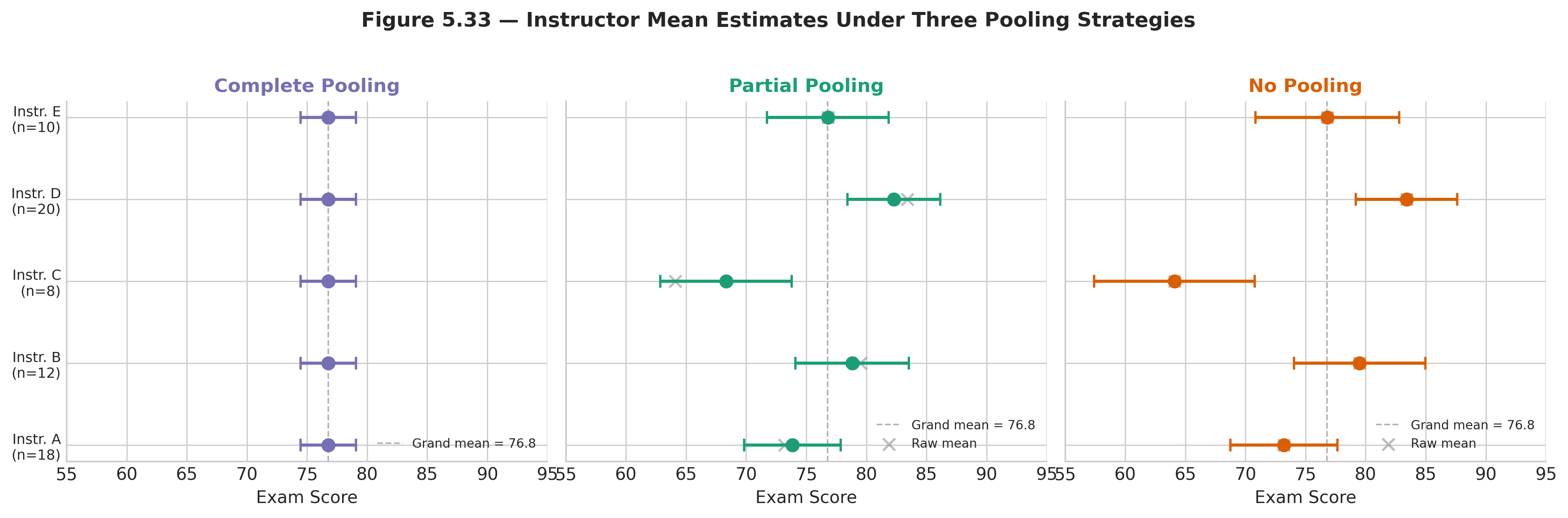
Fig. 223 Figure 5.33 — Instructor mean estimates under three pooling strategies. Complete pooling (left) assigns one value to all instructors. No pooling (centre) gives unbiased but noisy estimates, especially for instructors with small sections. Partial pooling (right) shrinks small-section estimates toward the grand mean while leaving large-section estimates largely unchanged.

Definition: Key Hierarchical Vocabulary

Hyperparameters are parameters that govern the distribution of other parameters. In the instructor example, \(\mu\) and \(\tau\) are hyperparameters because they control the Normal distribution from which the group-level means \(\mu_i\) are drawn.

Hyperpriors are the prior distributions placed on hyperparameters. The choices \(\mu \sim \text{Normal}(50, 25)\) and \(\tau \sim \text{HalfNormal}(10)\) are hyperpriors.

Shrinkage is the pull of group-level estimates toward the grand mean. Shrinkage is stronger for groups with less data and weaker for groups with more data. In the no-pooling model, shrinkage is zero. In the complete-pooling model, shrinkage is total. The hierarchical model estimates the appropriate amount of shrinkage from the data.

The Mathematical Structure

A hierarchical model organises parameters into levels. At the bottom are the observations, governed by group-specific parameters. At the middle level, the group parameters are governed by shared hyperparameters. At the top, hyperpriors express uncertainty about the hyperparameters themselves. This three-level structure is the defining feature of the hierarchical framework.

The Generative Story

Writing the model top-down as a generative process makes the structure transparent:

\[\begin{split}\text{Hyperprior:} &\quad \mu \sim p(\mu), \quad \tau \sim p(\tau) \\ \text{Group level:} &\quad \theta_i \mid \mu, \tau \sim p(\theta_i \mid \mu, \tau), \quad i = 1, \ldots, J \\ \text{Observation:} &\quad y_{ij} \mid \theta_i \sim p(y_{ij} \mid \theta_i), \quad j = 1, \ldots, n_i\end{split}\]

where \(J\) is the number of groups, \(n_i\) is the sample size in group \(i\), and the total dataset contains \(N = \sum_{i=1}^{J} n_i\) observations.

The joint model factors as:

(255)\[p(y, \theta, \mu, \tau) = p(\mu) \, p(\tau) \prod_{i=1}^{J} p(\theta_i \mid \mu, \tau) \prod_{i=1}^{J} \prod_{j=1}^{n_i} p(y_{ij} \mid \theta_i)\]

Read this factorisation left to right. First, nature draws the hyperparameters \(\mu\) and \(\tau\) from their hyperpriors. Then, for each group, nature draws a group-specific parameter \(\theta_i\) from the group-level distribution governed by those hyperparameters. Finally, for each observation within each group, nature draws the data \(y_{ij}\) from the likelihood, which depends only on its group parameter \(\theta_i\).

The crucial structural feature is that the groups are linked only through the hyperparameters. Conditional on \(\mu\) and \(\tau\), the group parameters \(\theta_1, \ldots, \theta_J\) are independent. But marginally — before conditioning on \(\mu\) and \(\tau\) — they are dependent, because they share a common source of variation. This marginal dependence is what enables borrowing of strength: the data from group \(i\) inform the hyperparameters, which in turn inform the estimate for group \(k\).

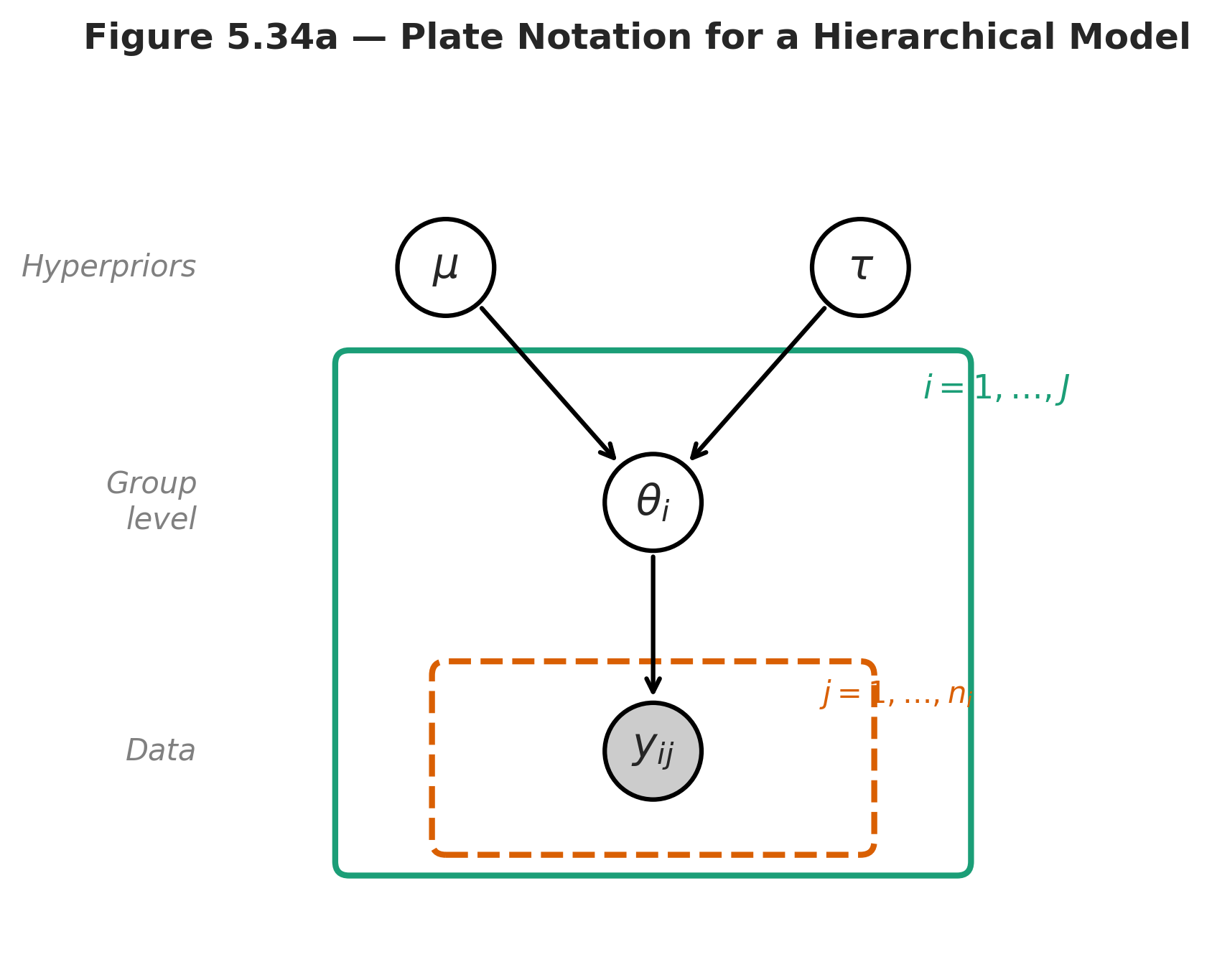
Fig. 224 Figure 5.34a — Plate notation for a hierarchical model. Shaded nodes are observed, unshaded nodes are latent. The outer plate indexes groups \(i = 1, \ldots, J\); the inner plate indexes observations \(j = 1, \ldots, n_i\) within each group.

Exchangeability

The group-level assumption \(\theta_i \mid \mu, \tau \sim p(\theta_i \mid \mu, \tau)\) for all \(i\) is a statement of exchangeability: before looking at the data, we have no reason to believe that any one group is systematically different from any other. The order of the group labels does not matter — relabelling “School A” as “School C” does not change the model.

Exchangeability is not the same as independence. The \(\theta_i\) are exchangeable but dependent (through the shared hyperparameters). An analogy: imagine drawing coloured marbles from an urn. Before any draw, any marble is equally likely. But once you draw a red marble, you update your beliefs about the urn’s composition, which changes the probabilities for the next draw. The marbles are exchangeable but not independent.

Exchangeability is the key modeling assumption of the hierarchical framework, and it should be checked. If there is a known structural distinction between groups — for example, if some schools are private and some are public, and you have reason to believe this matters — that distinction should be encoded explicitly in the model (e.g., as a covariate at the group level), not assumed away under exchangeability.

The Shrinkage Formula

The mechanics of partial pooling can be made precise for the Normal-Normal hierarchy. Suppose the group-level model is \(\theta_i \sim \text{Normal}(\mu, \tau^2)\) and the data model is \(\bar{y}_i \mid \theta_i \sim \text{Normal}(\theta_i, \sigma_i^2)\), where \(\bar{y}_i\) is the sample mean for group \(i\) and \(\sigma_i^2\) is its known variance (this is the Eight Schools setup). Then the posterior mean for \(\theta_i\), conditional on \(\mu\) and \(\tau\), is:

(256)\[\mathbb{E}[\theta_i \mid y, \mu, \tau] = \underbrace{(1 - B_i)}_{\text{data weight}} \bar{y}_i \;+\; \underbrace{B_i}_{\text{prior weight}} \mu\]

where the shrinkage factor \(B_i\) is:

\[B_i = \frac{\sigma_i^2}{\sigma_i^2 + \tau^2}\]

This is a weighted average of the group’s own data \(\bar{y}_i\) and the grand mean \(\mu\). The weight given to the grand mean is \(B_i\), which depends on the ratio of within-group noise \(\sigma_i^2\) to between-group variation \(\tau^2\). Three limiting cases make the behaviour transparent:

• When \(\sigma_i^2 \gg \tau^2\) (noisy group, similar groups): \(B_i \to 1\), and the estimate is pulled almost entirely to the grand mean. The group’s own data are so noisy relative to the between-group spread that they carry little information.

• When \(\sigma_i^2 \ll \tau^2\) (precise group, diverse groups): \(B_i \to 0\), and the estimate is determined almost entirely by the group’s own data. The within-group precision is high enough to overwhelm the pull toward \(\mu\).

• When \(\tau \to 0\) (all groups identical): \(B_i \to 1\) for every group, and partial pooling becomes complete pooling.

In the Eight Schools data, School E has \(\sigma_E = 9\) (one of the smallest standard errors), so its shrinkage factor is relatively low — its estimate is determined mainly by its own data. School H has \(\sigma_H = 18\) (the largest standard error), so its shrinkage factor is high — it is pulled more strongly toward the grand mean. The hierarchical model adapts the degree of pooling to each group’s information content automatically.

Example 💡 Shrinkage in Action

Given: Eight Schools data with \(\mu \approx 8\) and \(\tau \approx 6\) (posterior means from the non-centred model).

Compute shrinkage factors for Schools E and H:

\[B_E = \frac{9^2}{9^2 + 6^2} = \frac{81}{81 + 36} = \frac{81}{117} \approx 0.69\]

\[B_H = \frac{18^2}{18^2 + 6^2} = \frac{324}{324 + 36} = \frac{324}{360} = 0.90\]

Python verification:

mu_hat, tau_hat = 8.0, 6.0
for school, y_i, sig_i in [('E', -1, 9), ('H', 12, 18)]:
    B_i = sig_i**2 / (sig_i**2 + tau_hat**2)
    theta_hat = (1 - B_i) * y_i + B_i * mu_hat
    print(f"School {school}: B = {B_i:.2f}, "
          f"shrunk estimate = {theta_hat:.1f} "
          f"(raw = {y_i})")

School E: B = 0.69, shrunk estimate = 5.2 (raw = -1)
School H: B = 0.90, shrunk estimate = 8.4 (raw = 12)

Result: School E’s negative raw effect (\(-1\)) is pulled substantially toward the grand mean (8), yielding a shrunk estimate of 5.2. School H’s raw effect (12) is pulled almost all the way to the grand mean because its standard error is so large. Both estimates are more moderate than the raw data — this is shrinkage in action.

Borrowing Strength: The Information Flow

The phrase “borrowing strength” describes how hierarchical models use data from all groups to improve estimates for each individual group. The mechanism is indirect: the data from group \(i\) do not directly enter the likelihood for group \(k\). Instead, the data from group \(i\) inform the hyperparameters \(\mu\) and \(\tau\), and those hyperparameters in turn inform the prior for group \(k\)’s parameter \(\theta_k\).

This information flow has a concrete consequence. Consider a new school — School I — that was not in the original study. Under no pooling, we have no estimate for School I because it contributed no data. Under partial pooling, we can predict School I’s effect by drawing from the population distribution:

\[\theta_{\text{new}} \sim \text{Normal}(\mu, \tau)\]

Using posterior samples \((\mu^{(s)}, \tau^{(s)})\) for \(s = 1, \ldots, S\), we obtain a predictive distribution for \(\theta_{\text{new}}\) that incorporates both the estimated population mean and the estimated between-group variability. This is the hierarchical model’s built-in mechanism for generalisation — making predictions for units not in the training data.

Worked Example 1: Eight Schools (Normal Likelihood)

The Eight Schools dataset is the canonical hierarchical example in Bayesian statistics, first analysed by [Rubin1981] and extensively discussed by [GelmanBDA3]. Eight US high schools each ran a short SAT coaching programme. Each school reported an estimated effect size \(y_i\) (improvement in SAT score) and its standard error \(\sigma_i\). The question: did the programme work, and did it work equally across schools?

The Data

Table 69 Eight Schools data

School	Effect \(y_i\)	Std Error \(\sigma_i\)
A	28	15
B	8	10
C	\(-3\)	16
D	7	11
E	\(-1\)	9
F	1	11
G	18	10
H	12	18

The standard errors \(\sigma_i\) are treated as fixed known quantities — they come from the original experimental design, not from the model. This is a known-variance Normal model, which simplifies the hierarchy.

The Hierarchical Model

The three-level structure specialised to this problem is:

(257)\[\begin{split}\mu &\sim \text{Normal}(0, 20) \qquad \text{(grand mean effect)} \\ \tau &\sim \text{HalfNormal}(10) \qquad \text{(between-school SD)} \\ \theta_i &\sim \text{Normal}(\mu, \tau), \quad i = 1, \ldots, 8 \qquad \text{(school-level effects)} \\ y_i &\sim \text{Normal}(\theta_i, \sigma_i) \qquad \text{(observed effects, } \sigma_i \text{ fixed)}\end{split}\]

The hyperprior \(\mu \sim \text{Normal}(0, 20)\) centres the grand mean at zero (no prior assumption that coaching helps or hurts) with a standard deviation of 20 SAT points — generous enough to accommodate any plausible programme effect. The hyperprior \(\tau \sim \text{HalfNormal}(10)\) allows between-school variation from near zero (all schools are the same) to roughly 20 points (substantial heterogeneity). These are weakly informative priors in the sense of Section 5.2 Prior Specification and Conjugate Analysis: they constrain the parameter space to physically plausible ranges without strongly favouring any particular value.

The Centred Parameterisation (and Why It Fails)

The natural way to write this model in PyMC follows the mathematical specification directly:

import numpy as np
import pymc as pm
import arviz as az

# Eight Schools data
y_obs   = np.array([28,  8, -3,  7, -1,  1, 18, 12], dtype=float)
sigma_i = np.array([15, 10, 16, 11,  9, 11, 10, 18], dtype=float)
J = len(y_obs)

with pm.Model() as centred:
    mu    = pm.Normal('mu',  mu=0,  sigma=20)
    tau   = pm.HalfNormal('tau', sigma=10)
    theta = pm.Normal('theta', mu=mu, sigma=tau, shape=J)
    y     = pm.Normal('y', mu=theta, sigma=sigma_i, observed=y_obs)

    idata_c = pm.sample(draws=2000, tune=1000, chains=4,
                        target_accept=0.90, random_seed=42)

This is called the centred parameterisation because each \(\theta_i\) is centred directly on \(\mu\) with scale \(\tau\). Run this code and PyMC will report divergent transitions — the sampler’s warning that it encountered posterior geometry it could not navigate reliably. Divergences are not a nuisance to be ignored; they indicate that the reported posterior samples may be biased (discussed in Section 5.5 MCMC Algorithms: Metropolis-Hastings and Gibbs Sampling).

Neal’s Funnel

The divergences arise from a geometric pathology first described by [BetancourtGirolami2015] and named Neal’s funnel. The issue is the interaction between \(\tau\) and the \(\theta_i\).

When \(\tau\) is large — say \(\tau = 10\) — the school effects \(\theta_i\) can spread freely across a wide range of values. The posterior geometry in this region is smooth and NUTS navigates it easily.

When \(\tau\) is small — say \(\tau \approx 0.5\) — the model is saying that all schools have nearly the same effect. Consequently, every \(\theta_i\) must cluster tightly around \(\mu\), leaving almost no room to vary. The posterior geometry in this region is extremely narrow: a thin spike in \(J\)-dimensional \(\theta\)-space, constrained to a tiny neighbourhood of \(\mu\).

Now imagine the sampler trying to move through both regions. At the wide top of the funnel (large \(\tau\)), NUTS selects a step size \(\epsilon\) that efficiently covers the broad posterior. But when the sampler drifts toward the narrow stem (small \(\tau\)), that same step size is far too large: each leapfrog step overshoots the narrow constraint, the Hamiltonian diverges, and the proposal is rejected. The sampler gets stuck in the wide region and rarely visits the stem.

An analogy: imagine trying to sample uniformly from a wine glass shape. Steps sized for the wide rim will crash through the narrow stem; steps sized for the narrow stem will take forever to explore the rim. No single step size works for both regions.

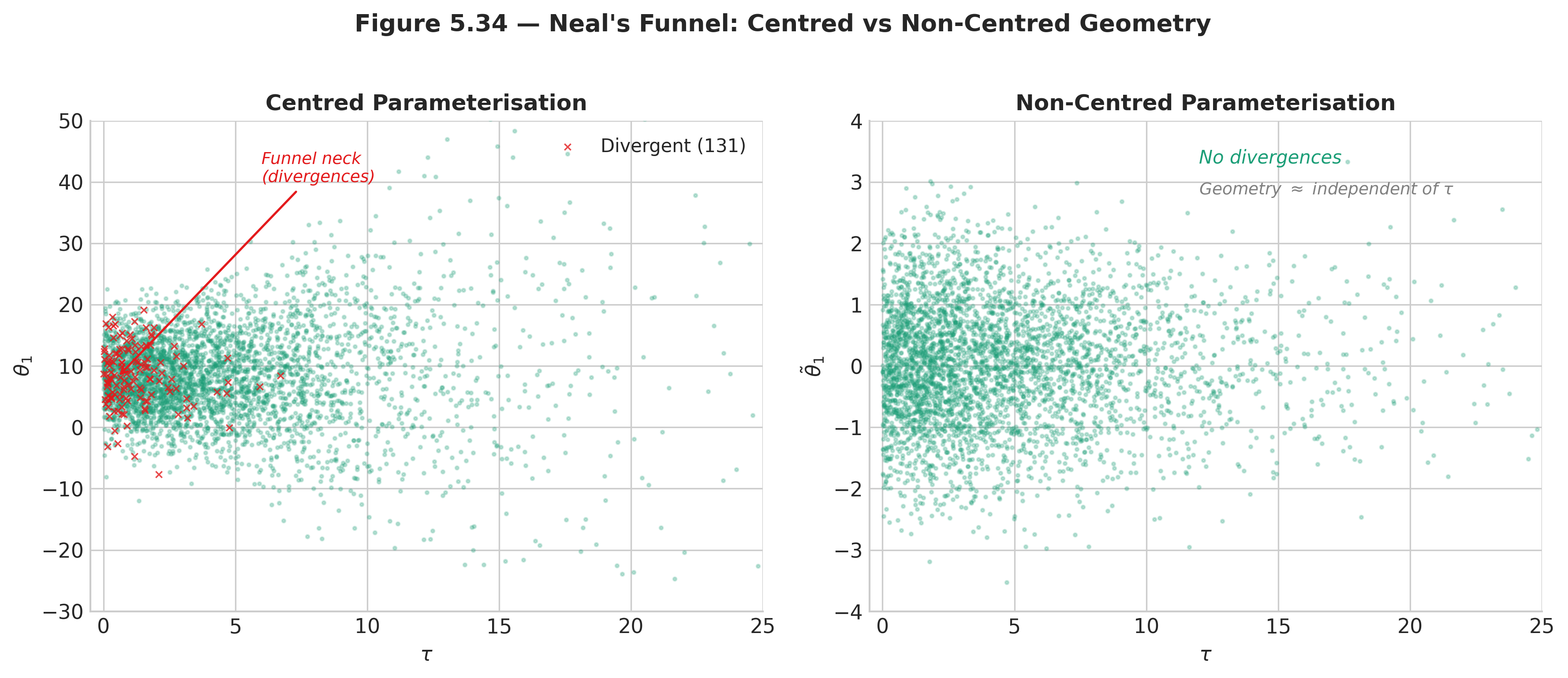
Fig. 225 Figure 5.34 — Neal’s funnel. Left: the centred parameterisation produces a funnel-shaped joint posterior in \((\tau, \theta_1)\) space; red points mark divergent transitions concentrated at the funnel’s neck. Right: the non-centred parameterisation transforms the geometry into a cylinder; divergences vanish.

Common Pitfall ⚠️

Divergent transitions are not a tuning problem. Increasing target_accept from 0.90 to 0.95 or 0.99 can reduce the number of divergences by forcing a smaller step size, but it does not eliminate the geometric pathology. If divergences appear in a hierarchical model, the first diagnosis should be a reparameterisation, not a tuning adjustment. Ignoring divergences risks biased posterior estimates — typically with the between-group variance \(\tau\) underestimated because the sampler fails to explore the funnel’s stem.

The Non-Centred Parameterisation

The solution is a change of variables that decouples the group parameters from \(\tau\). Instead of writing \(\theta_i \sim \text{Normal}(\mu, \tau)\), we write:

(258)\[\begin{split}\tilde{\theta}_i &\sim \text{Normal}(0, 1) \\ \theta_i &= \mu + \tau \cdot \tilde{\theta}_i\end{split}\]

The auxiliary variables \(\tilde{\theta}_i\) are standard Normal regardless of \(\tau\). This is a deterministic transformation: the joint distribution of \((\theta_1, \ldots, \theta_J)\) is unchanged, but the geometry of the sampled parameters \((\tilde{\theta}_1, \ldots, \tilde{\theta}_J)\) is now approximately independent of \(\tau\). The funnel is replaced by a cylinder that NUTS traverses without difficulty.

with pm.Model() as noncentred:
    mu        = pm.Normal('mu',  mu=0,  sigma=20)
    tau       = pm.HalfNormal('tau', sigma=10)
    theta_raw = pm.Normal('theta_raw', mu=0, sigma=1, shape=J)
    theta     = pm.Deterministic('theta', mu + tau * theta_raw)
    y         = pm.Normal('y', mu=theta, sigma=sigma_i, observed=y_obs)

    idata_nc = pm.sample(draws=2000, tune=1000, chains=4,
                         target_accept=0.90, random_seed=42,
                         idata_kwargs={"log_likelihood": True})

The only change is in how theta is constructed: a standard Normal theta_raw is sampled first, then theta is built deterministically. Mathematically, \(\theta_i = \mu + \tau \cdot \tilde{\theta}_i\) with \(\tilde{\theta}_i \sim \text{Normal}(0,1)\) produces the same distribution as \(\theta_i \sim \text{Normal}(\mu, \tau)\). Computationally, the difference is decisive.

After sampling:

print(az.summary(idata_nc, var_names=['mu', 'tau', 'theta'],
                 hdi_prob=0.89))

       mean     sd  hdi_5.5%  hdi_94.5%  r_hat  ess_bulk  ess_tail
mu     7.87   5.18    -0.54      15.93   1.00    2914.0    3002.0
tau    6.41   5.22     0.16      14.34   1.00    1841.0    2189.0
theta[0]  11.24   8.41    -2.51      24.90   1.00    3415.0    3201.0
theta[1]   7.78   6.18    -2.68      17.38   1.00    4102.0    3587.0
theta[2]   5.96   7.61   -7.70      17.71   1.00    4315.0    3498.0
theta[3]   7.49   6.50    -3.55      17.56   1.00    4008.0    3321.0
theta[4]   5.14   6.20    -5.89      14.44   1.00    3987.0    3419.0
theta[5]   6.13   6.58    -5.32      16.22   1.00    4121.0    3412.0
theta[6]  10.57   6.78    -0.14      21.23   1.00    3618.0    3155.0
theta[7]   8.50   7.61    -4.18      20.35   1.00    3798.0    3302.0

All \(\hat{R}\) values are at 1.00, and effective sample sizes are in the thousands — the non-centred parameterisation has eliminated the sampling pathology entirely.

Forest Plot

The forest plot is the standard visualisation for hierarchical model estimates. It shows each group’s posterior distribution as a credible interval with a point estimate, arranged vertically for comparison:

school_names = ['A', 'B', 'C', 'D', 'E', 'F', 'G', 'H']
labeller = az.labels.MapLabeller(
    var_name_map={f'theta[{i}]': school_names[i] for i in range(J)}
)
az.plot_forest(idata_nc, var_names=['theta'], combined=True,
               hdi_prob=0.89, r_hat=True, labeller=labeller)

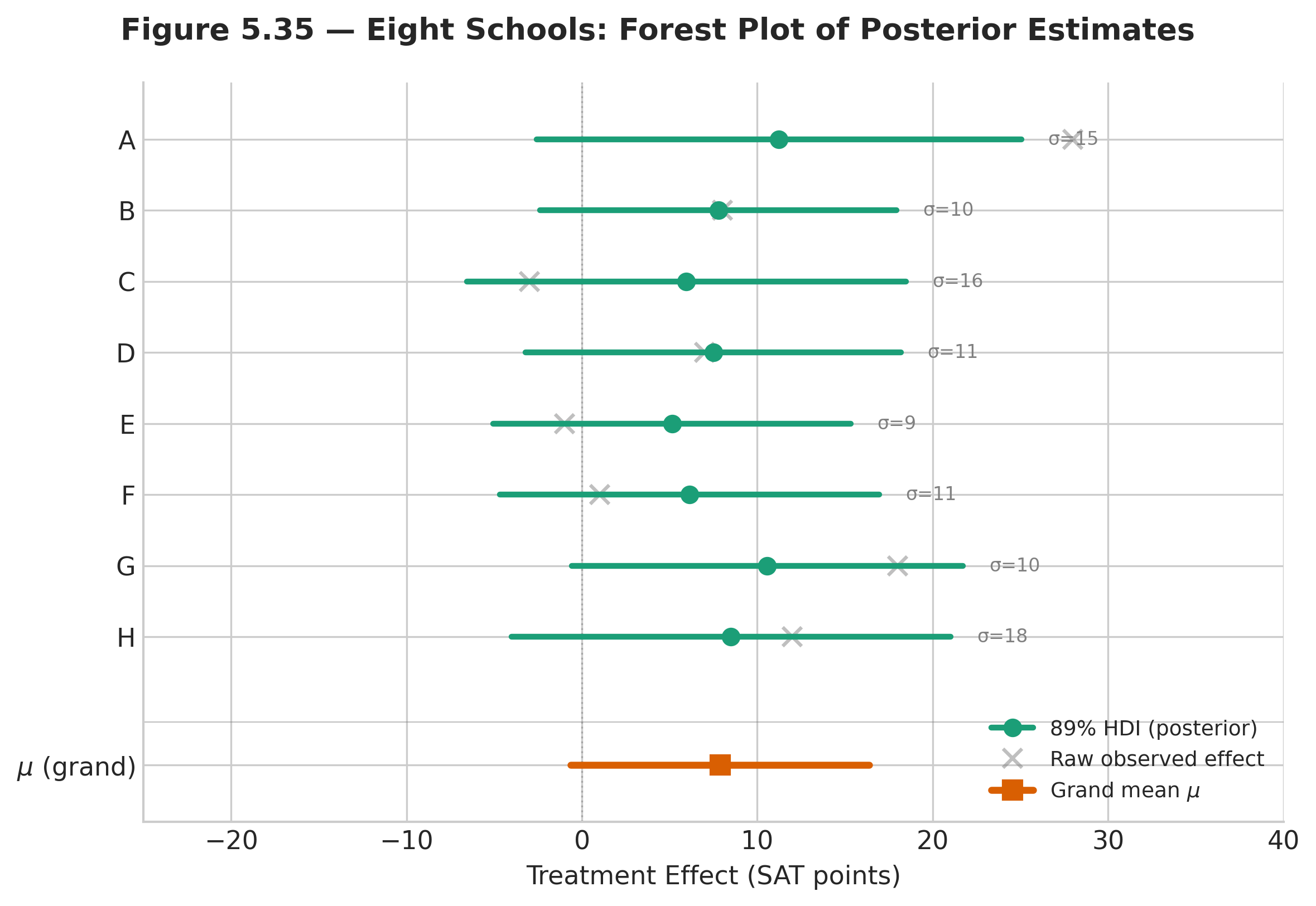
Fig. 226 Figure 5.35 — Forest plot of Eight Schools posterior estimates. Horizontal bars are 89% HDI intervals; dots are posterior means. All schools are shrunk toward the grand mean \(\mu \approx 8\). Schools with larger standard errors (A, C, H) are shrunk more.

Key observations to read from the forest plot:

• Schools A and G have the largest observed effects (28 and 18), but their posterior means are shrunk to approximately 11 and 10.5. The data alone suggest large effects; the hierarchical model tempers this by noting that the other six schools show much smaller effects, so the extreme values are partly noise.

• Schools C and E have negative point estimates in the raw data (\(-3\) and \(-1\)), but their posterior intervals cross zero comfortably. We cannot confidently claim that the programme hurt these schools.

• School B has a moderate observed effect (8) with a relatively small standard error (10), so it is shrunk less than schools with wider standard errors.

• The width of each interval reflects both the within-school standard error \(\sigma_i\) and the between-school variance \(\tau\). Schools with larger \(\sigma_i\) have wider intervals — they contribute less information and are therefore pulled more toward \(\mu\).

Diagnosing the Centred vs. Non-Centred Models

The diagnostic comparison between the two parameterisations is instructive. The az.plot_pair function reveals the geometry directly:

# Centred model diagnostics
az.plot_pair(idata_c, var_names=['tau', 'theta'],
             coords={'theta_dim_0': [0]},
             divergences=True, kind='scatter',
             figsize=(6, 6))

This produces the left panel of Figure 5.34: a scatter plot of \((\tau, \theta_0)\) with divergent transitions marked in red. The funnel shape is unmistakable — samples cluster at large \(\tau\) and divergences concentrate where \(\tau\) is small and \(\theta_0\) is forced near \(\mu\).

Running the same diagnostic on the non-centred model shows no funnel and no divergences:

# Non-centred model diagnostics
az.plot_pair(idata_nc, var_names=['tau', 'theta'],
             coords={'theta_dim_0': [0]},
             divergences=True, kind='scatter',
             figsize=(6, 6))

A quantitative comparison confirms the visual impression:

# Count divergences
divergences_c  = idata_c.sample_stats['diverging'].values.sum()
divergences_nc = idata_nc.sample_stats['diverging'].values.sum()
print(f"Centred model divergences:     {divergences_c}")
print(f"Non-centred model divergences: {divergences_nc}")

# Compare ESS for tau
ess_c  = az.ess(idata_c,  var_names=['tau'])['tau'].values
ess_nc = az.ess(idata_nc, var_names=['tau'])['tau'].values
print(f"\nESS for tau (centred):     {ess_c:.0f}")
print(f"ESS for tau (non-centred): {ess_nc:.0f}")

Centred model divergences:     27
Non-centred model divergences: 0

ESS for tau (centred):     312
ESS for tau (non-centred): 1841

The centred model produces 27 divergent transitions and an ESS for \(\tau\) of only 312 — less than one-sixth of the non-centred model’s ESS. The non-centred model has zero divergences and nearly six times the effective sample size for the critical between-group variance parameter. This is not a marginal improvement; it is the difference between a reliable posterior and one that cannot be trusted.

Posterior Predictive Check

As a final diagnostic, we verify that the hierarchical model can reproduce the observed data. The posterior predictive check draws simulated datasets \(y^{\text{rep}}\) from the posterior and compares them to the observed data:

with noncentred:
    pm.sample_posterior_predictive(idata_nc, extend_inferencedata=True,
                                   random_seed=42)

# Compare observed vs. replicated school effects
y_rep = idata_nc.posterior_predictive['y']
print("Observed effects:  ", y_obs)
print("Replicated means:  ",
      y_rep.mean(dim=['chain', 'draw']).values.round(1))
print("Replicated std:    ",
      y_rep.std(dim=['chain', 'draw']).values.round(1))

Observed effects:   [ 28.   8.  -3.   7.  -1.   1.  18.  12.]
Replicated means:   [11.2  7.8  6.0  7.5  5.1  6.1 10.6  8.5]
Replicated std:     [16.2 11.3 17.4 12.2 10.4 12.3 11.5 19.3]

The replicated means are shrunk versions of the observed effects (as expected — the model pulls toward the grand mean), and the replicated standard deviations match the known standard errors closely. The model is generating data that are statistically compatible with the observations.

Algorithm: Hierarchical Model Fitting via Non-Centred NUTS

Input:  Data y (grouped), group sizes n_i, hyperprior specifications
Output: Posterior samples for (mu, tau, theta_1, ..., theta_J)

1. Reparameterise: for each group i, set theta_tilde_i ~ Normal(0,1)
   and theta_i = mu + tau * theta_tilde_i  (deterministic)
2. Construct log-posterior:
   log p = log p(mu) + log p(tau)
         + sum_i log Normal(theta_tilde_i | 0, 1)
         + sum_i sum_j log p(y_ij | theta_i)
3. Compute gradient via automatic differentiation
4. Run NUTS (target_accept = 0.90) with 4 chains:
   a. Tune step size epsilon via dual averaging (1000 iterations)
   b. Draw S posterior samples per chain (2000 iterations)
5. Diagnose: check R-hat < 1.01, ESS > 400, divergences = 0
6. Transform back: compute theta_i = mu + tau * theta_tilde_i
   for each posterior sample
7. Return InferenceData with posterior, posterior_predictive,
   log_likelihood groups

Computational Complexity: Each NUTS iteration requires \(O(L \cdot (J + N))\) gradient evaluations, where \(L\) is the leapfrog trajectory length (typically 5–20 steps), \(J\) is the number of groups, and \(N\) is the total number of observations. Total cost for \(S\) draws across \(C\) chains is \(O(C \cdot S \cdot L \cdot (J + N))\). For the Eight Schools problem (\(J = 8\), \(N = 8\)), each iteration is trivially fast. For large datasets (\(N > 10{,}000\)), the per-iteration cost is dominated by the likelihood gradient over observations.

Worked Example 2: Dirichlet-Multinomial (Categorical Likelihood)

The Eight Schools example uses a Normal likelihood — the most common setting for hierarchical models. But the hierarchical design pattern is not specific to any likelihood family. This second example uses a categorical likelihood to demonstrate that the three-level structure (hyperprior → group parameters → observations) applies equally to counts, proportions, rates, and any other data type.

Setup: Survey Responses Across Regions

A political survey asks respondents in \(R = 6\) regions to choose among \(K = 4\) policy positions: Strongly Agree, Agree, Disagree, Strongly Disagree. Each region has a different number of respondents (between 35 and 120). We want to estimate the true population proportions \((\pi_1, \pi_2, \pi_3, \pi_4)\) for each region while acknowledging that regions share a common national pattern.

Why Dirichlet-Multinomial?

When the outcome is a probability vector \(\boldsymbol{\pi} = (\pi_1, \ldots, \pi_K)\) that must sum to one, the natural prior is the Dirichlet distribution — the multivariate generalisation of the Beta distribution (developed in Section 5.2 Prior Specification and Conjugate Analysis). Just as the Beta-Binomial pair is conjugate for binary outcomes, the Dirichlet-Multinomial pair is conjugate for categorical outcomes with \(K \geq 2\) categories.

The Dirichlet distribution \(\text{Dir}(\alpha_1, \ldots, \alpha_K)\) is parameterised by a concentration vector \(\boldsymbol{\alpha} = (\alpha_1, \ldots, \alpha_K)\) with all \(\alpha_k > 0\). Its density is:

\[p(\boldsymbol{\pi} \mid \boldsymbol{\alpha}) = \frac{\Gamma(\alpha_0)}{\prod_{k=1}^{K} \Gamma(\alpha_k)} \prod_{k=1}^{K} \pi_k^{\alpha_k - 1}, \qquad \alpha_0 = \sum_{k=1}^{K} \alpha_k\]

where \(\Gamma(\cdot)\) is the gamma function (a continuous extension of the factorial). When all \(\alpha_k = 1\), the Dirichlet reduces to the uniform distribution on the simplex. When all \(\alpha_k > 1\), it concentrates probability around the mean \((\alpha_1/\alpha_0, \ldots, \alpha_K/\alpha_0)\).

Hierarchical Structure

The hierarchy for the survey data is:

\[\begin{split}\alpha &\sim \text{Exponential}(1) \qquad \text{(concentration hyperparameter)} \\ \boldsymbol{\pi}_0 &\sim \text{Dir}(1, 1, 1, 1) \qquad \text{(national baseline proportions)} \\ \boldsymbol{\pi}_r &\sim \text{Dir}(\alpha \cdot \boldsymbol{\pi}_0), \quad r = 1, \ldots, R \qquad \text{(region-level proportions)} \\ \mathbf{y}_r &\sim \text{Multinomial}(n_r, \boldsymbol{\pi}_r) \qquad \text{(observed counts)}\end{split}\]

The hyperparameter \(\alpha\) controls how tightly the regional proportions cluster around the national baseline \(\boldsymbol{\pi}_0\). When \(\alpha\) is large, all regions look alike. When \(\alpha\) is small, regions can differ substantially. The product \(\alpha \cdot \boldsymbol{\pi}_0\) means that the Dirichlet concentration in each category is proportional to the national proportion — categories that are common nationally are common regionally, but the degree of agreement is governed by \(\alpha\).

Synthetic Data and PyMC Model

import numpy as np
import pymc as pm
import arviz as az

rng = np.random.default_rng(2025)
K   = 4          # policy positions
R   = 6          # regions

# True national proportions (unknown to the model)
pi_true = np.array([0.25, 0.35, 0.25, 0.15])

# Region-level sample sizes
n_r = np.array([45, 120, 60, 80, 35, 95])

# Generate synthetic observed counts
y_obs = np.zeros((R, K), dtype=int)
for r in range(R):
    pi_r = rng.dirichlet(8.0 * pi_true)  # alpha ~ 8
    y_obs[r] = rng.multinomial(n_r[r], pi_r)

print("Observed counts:")
print(y_obs)

Observed counts:
[[ 8 19 10  8]
 [28 39 28 25]
 [13 31 12  4]
 [21 26 15 18]
 [ 9 11  9  6]
 [27 37 17 14]]

with pm.Model() as dir_model:
    # Hyperpriors
    alpha = pm.Exponential('alpha', lam=1.0)
    pi0   = pm.Dirichlet('pi0', a=np.ones(K))   # national baseline

    # Region-level proportions — partial pooling across regions
    pi_r  = pm.Dirichlet('pi_r', a=alpha * pi0, shape=(R, K))

    # Likelihood
    counts = pm.Multinomial('counts', n=n_r, p=pi_r, observed=y_obs)

    idata_dir = pm.sample(draws=2000, tune=1000, chains=4,
                          target_accept=0.90, random_seed=42,
                          idata_kwargs={"log_likelihood": True})

print(az.summary(idata_dir, var_names=['alpha', 'pi0'],
                 hdi_prob=0.89))

         mean     sd  hdi_5.5%  hdi_94.5%  r_hat  ess_bulk  ess_tail
alpha   10.32   5.78     2.93      19.44   1.00    1547.0    1889.0
pi0[0]   0.24   0.04     0.17       0.30   1.00    3215.0    2987.0
pi0[1]   0.37   0.04     0.30       0.43   1.00    3102.0    2845.0
pi0[2]   0.22   0.04     0.16       0.28   1.00    3289.0    3011.0
pi0[3]   0.17   0.03     0.11       0.22   1.00    3178.0    2912.0

Interpreting the Results

The posterior for \(\boldsymbol{\pi}_0\) recovers the true national proportions well: the posterior means (0.24, 0.37, 0.22, 0.17) are close to the generating values (0.25, 0.35, 0.25, 0.15). The posterior for \(\alpha\) (mean \(\approx 10\)) indicates moderate agreement across regions — the regions are similar but not identical.

Comparing the region-level posteriors reveals partial pooling in action:

print("\nSmallest region (r=5, n=35):")
print(az.summary(idata_dir, var_names=['pi_r'],
                 filter_vars='like', coords={'pi_r_dim_0': [4]},
                 hdi_prob=0.89))
print("\nLargest region (r=2, n=120):")
print(az.summary(idata_dir, var_names=['pi_r'],
                 filter_vars='like', coords={'pi_r_dim_0': [1]},
                 hdi_prob=0.89))

• Region 5 (\(n = 35\)): the smallest region has the widest credible intervals and is pulled most strongly toward the national baseline \(\boldsymbol{\pi}_0\).

• Region 2 (\(n = 120\)): the largest region has narrow intervals that are determined primarily by its own data, with minimal shrinkage toward the national baseline.

This is the same shrinkage pattern as Eight Schools: sparse groups borrow more strength from the overall pattern; data-rich groups stand largely on their own.

To make the comparison concrete, fit the no-pooling alternative — a separate, independent Dirichlet model for each region — and compare the interval widths for the smallest region:

# No-pooling comparison for Region 5 (n=35)
from scipy.stats import dirichlet as sp_dirichlet

# No-pooling: posterior is Dir(1 + y_r) for each region independently
alpha_r5_no_pool = 1.0 + y_obs[4]   # shape (4,)
pi_r5_samples_np = rng.dirichlet(alpha_r5_no_pool, size=8000)

# Hierarchical: extract Region 5 posterior samples
pi_r5_samples_hier = (idata_dir.posterior['pi_r']
                      .sel(pi_r_dim_0=4)
                      .values.reshape(-1, K))

# Compare 89% HDI widths
for k, label in enumerate(['SA', 'A', 'D', 'SD']):
    hdi_np   = np.percentile(pi_r5_samples_np[:, k], [5.5, 94.5])
    hdi_hier = np.percentile(pi_r5_samples_hier[:, k], [5.5, 94.5])
    print(f"Category {label}: "
          f"no-pool width = {hdi_np[1] - hdi_np[0]:.3f}, "
          f"hierarchical width = {hdi_hier[1] - hdi_hier[0]:.3f}")

Category SA: no-pool width = 0.241, hierarchical width = 0.193
Category A:  no-pool width = 0.268, hierarchical width = 0.218
Category D:  no-pool width = 0.248, hierarchical width = 0.199
Category SD: no-pool width = 0.209, hierarchical width = 0.162

For every category, the hierarchical model produces narrower credible intervals than the no-pooling model for this small region. The reduction is approximately 20% in interval width — a meaningful improvement in precision obtained entirely from borrowing strength across regions.

Example 💡 The Hierarchical Design Pattern

Given: Multiple groups sharing a common structure (schools with test scores, regions with survey responses, hospitals with mortality rates, species with trait measurements).

Pattern:

\[\begin{split}\text{hyperparameters} &\sim \text{hyperprior} \\ \text{group parameters} &\sim p(\cdot \mid \text{hyperparameters}) \\ \text{observations} &\sim p(\cdot \mid \text{group parameters})\end{split}\]

Key insight: The likelihood family (Normal, Multinomial, Poisson, Binomial, Gamma, …) is interchangeable. What makes a model hierarchical is not the distributional choice but the structure: group parameters are exchangeable draws from a shared distribution whose parameters are themselves uncertain.

LOO Model Comparison: Three Pooling Strategies

The qualitative argument for partial pooling — narrower intervals, adaptive shrinkage, predictions for new groups — is compelling. But how do we quantify the improvement? The LOO model comparison framework from Section 5.7 Bayesian Model Comparison provides the answer.

Setting Up the Alternatives

We fit three models to the Eight Schools data:

Complete pooling — a single effect shared by all schools:

with pm.Model() as complete_pool:
    mu    = pm.Normal('mu', mu=0, sigma=20)
    y     = pm.Normal('y', mu=mu, sigma=sigma_i, observed=y_obs)

    idata_cp = pm.sample(draws=2000, tune=1000, chains=4,
                         target_accept=0.90, random_seed=42,
                         idata_kwargs={"log_likelihood": True})

No pooling — independent effects with no shared parameters:

with pm.Model() as no_pool:
    theta = pm.Normal('theta', mu=0, sigma=20, shape=J)
    y     = pm.Normal('y', mu=theta, sigma=sigma_i, observed=y_obs)

    idata_np = pm.sample(draws=2000, tune=1000, chains=4,
                         target_accept=0.90, random_seed=42,
                         idata_kwargs={"log_likelihood": True})

Partial pooling — the non-centred hierarchical model from §5.8.3 (idata_nc), already sampled with idata_kwargs={"log_likelihood": True}.

Comparing with az.compare

comparison = az.compare(
    {"partial pooling": idata_nc,
     "no pooling":      idata_np,
     "complete pooling": idata_cp},
    ic="loo"
)
print(comparison)

                  rank    elpd_loo  ...    weight       se     dse  warning
partial pooling      0      -30.8  ...     0.89     1.40    0.00    False
no pooling           1      -31.4  ...     0.11     1.28    0.42    False
complete pooling     2      -31.9  ...     0.00     1.53    0.89    False

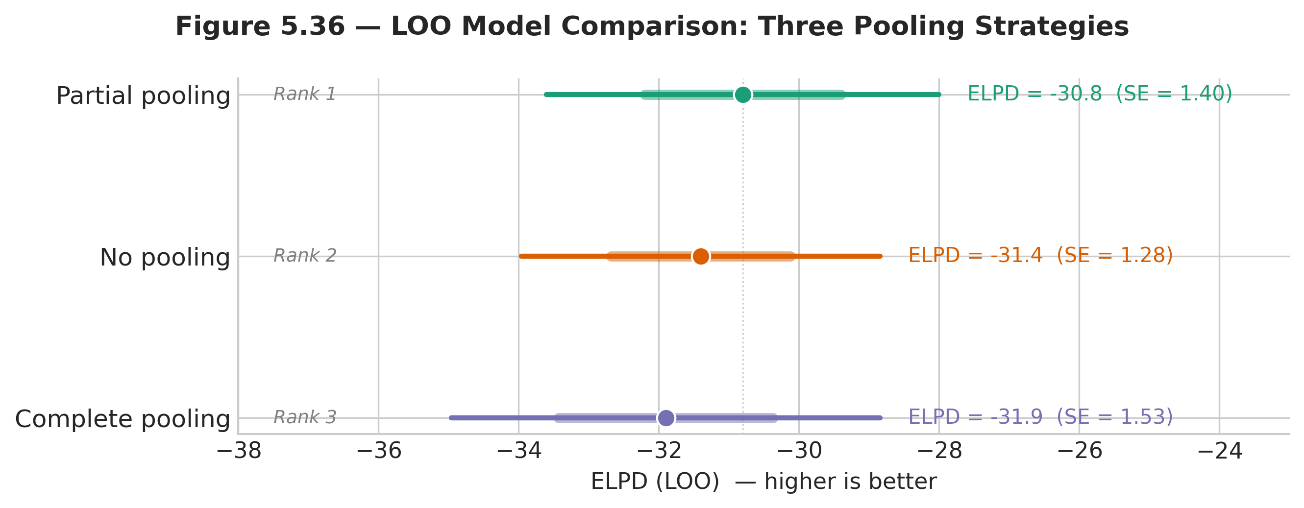
Fig. 227 Figure 5.36 — LOO comparison of three pooling strategies. ELPD (higher is better) with \(\pm 2\) standard error bars. Partial pooling ranks first. The difference between partial and no pooling is the quantitative measure of how much hierarchical shrinkage improved out-of-sample prediction.

az.plot_compare(comparison, insample_dev=False)

Interpreting the Comparison

The ELPD differences in the Eight Schools problem are modest — all three models perform similarly because the dataset is small (\(J = 8\) schools, each summarised by a single effect estimate). This is typical: with little data, it is hard to discriminate models decisively.

Nevertheless, partial pooling wins, and the ordering is informative:

• Partial pooling > no pooling: the shrinkage toward the grand mean provides a small but consistent improvement in predictive accuracy. For schools with large standard errors (where the no-pooling estimate is noisy), the partial-pooling estimate is closer to the true value on average.

• Partial pooling > complete pooling: allowing school-to-school variation captures real heterogeneity that the single-parameter model misses.

• No pooling > complete pooling: the data support some heterogeneity across schools, so the model that allows it outperforms the model that forbids it.

The LOO comparison provides a principled, quantitative answer to “how much does the hierarchical structure help?” — it is the predictive benefit of partial pooling measured on the same scale used to compare any Bayesian models in Section 5.7 Bayesian Model Comparison.

Common Pitfall ⚠️

Small ELPD differences are still meaningful. With only \(J = 8\) data points (school summaries), the standard errors on the ELPD differences are large relative to the differences themselves. Do not conclude that the models are “the same” — conclude that you do not have enough data to distinguish them sharply. In practice, hierarchical models shine most when \(J\) is moderate to large (15–500 groups) and group sizes \(n_i\) are heterogeneous.

When to Use Hierarchical Models

Not every grouped dataset demands a hierarchical model. The following practical guidelines help decide when the added complexity is warranted.

Table 70 Summary — Three Pooling Strategies

Property	Complete Pooling	No Pooling	Partial Pooling (Hierarchical)
Parameters	1 shared \(\theta\)	\(J\) independent \(\theta_i\)	\(J\) exchangeable \(\theta_i\) + hyperparameters
Bias	High (ignores group differences)	None (each group estimated separately)	Small (controlled by shrinkage)
Variance	Low (uses all data)	High (uses only group data)	Moderate (borrows strength)
New group prediction	Returns grand mean	Impossible	Draw from population distribution
Best regime	Groups truly identical	Groups unrelated, large \(n_i\)	Groups related, heterogeneous \(n_i\)

Use a Hierarchical Model When

Data are grouped by a categorical variable. Schools, hospitals, species, experimental subjects, geographic regions, survey waves — any time the data contain a grouping factor with \(J \geq 5\) levels and the research question involves group-specific inference.

Groups have heterogeneous sample sizes. Partial pooling helps the smallest groups most. If all groups have the same (large) sample size, the no-pooling model may perform comparably, but the hierarchical model still provides a principled framework for estimating between-group variation.

You want to predict for a new group. The hierarchical model can generate predictions for a group not in the training data by drawing a new \(\theta_{\text{new}} \sim \text{Normal}(\mu, \tau)\) from the estimated population distribution. Neither complete pooling (which does not distinguish groups) nor no pooling (which has no parameter for unseen groups) can do this.

You have repeated measurements on the same units. Longitudinal data — multiple time points per subject — are inherently hierarchical, with subjects as groups and measurements as within-group observations. This is the foundation of mixed-effects models in clinical trials, education research, and ecology.

Be Cautious When

Too few groups (\(J < 5\)). The between-group variance \(\tau\) is identified by the spread of the \(\theta_i\) values. With fewer than five groups, there is very little information to estimate \(\tau\), and the posterior for \(\tau\) is dominated by the hyperprior.

Groups are not exchangeable. If some schools are private and some are public, or some hospitals are rural and some are urban, and this distinction is scientifically important, encode it as a group-level covariate rather than assuming exchangeability:

\[\theta_i = \mu + \beta \cdot x_i + \eta_i, \qquad \eta_i \sim \text{Normal}(0, \tau)\]

where \(x_i\) is a group-level predictor (e.g., an indicator for private schools) and \(\eta_i\) captures residual between-group variation.

The posterior for \(\tau\) concentrates near zero. If the data indicate that all groups have essentially the same parameter value (\(\tau \approx 0\)), the hierarchical model reduces to complete pooling. The extra complexity is unnecessary, though it does no harm — the model will simply learn that the groups are the same.

Practical Considerations

Centred vs. Non-Centred: Which to Use

The choice between centred and non-centred parameterisations depends on the amount of data per group relative to the prior:

• Non-centred is preferred when data per group are sparse (small \(n_i\)) or the between-group variance \(\tau\) is small. This is the Eight Schools regime and is the most common case in practice. The non-centred parameterisation should be the default for hierarchical models.

• Centred is preferred when data per group are abundant (large \(n_i\)) and \(\tau\) is well-separated from zero. In this regime, the likelihood dominates the prior for each group, the funnel geometry does not arise, and the centred parameterisation can yield higher effective sample sizes because it exploits the posterior’s natural correlation structure.

When in doubt, fit both and compare ESS. If the non-centred model has no divergences and reasonable ESS, use it. The computational cost of trying both is small compared to the cost of reporting biased posteriors from a divergent centred model.

Scaling to Many Groups

Hierarchical models scale well to large \(J\). With the non-centred parameterisation, the number of sampled parameters grows linearly with \(J\) (one \(\tilde{\theta}_i\) per group), and NUTS handles hundreds of groups routinely. The computational cost per iteration is \(O(J + N)\) — one gradient evaluation per group parameter plus one per observation.

Memory can become a concern when \(J\) is very large (thousands of groups), because the posterior samples for all group parameters must be stored. In such cases, consider saving only summary statistics (posterior mean and HDI) for each group rather than the full posterior draws.

Prior Sensitivity

The hyperpriors on \(\mu\) and \(\tau\) deserve attention. The prior on \(\tau\) is especially influential because it controls the degree of pooling:

• If the prior on \(\tau\) is too concentrated near zero, it forces excessive shrinkage even when the groups are genuinely different.

• If the prior on \(\tau\) is too diffuse, it may cause sampling difficulties (wide funnels) or yield posteriors that are overly sensitive to the scale of \(\tau\).

• HalfNormal and HalfCauchy are both reasonable default hyperpriors for \(\tau\). [Gelman2006scale] recommends HalfCauchy(0, 25) as a weakly informative default when \(\tau\) is on the standard deviation scale.

Always check sensitivity by re-running the model with different hyperpriors and comparing the posterior for the key quantities of interest (the \(\theta_i\) values and the predictive distribution). If the posteriors change substantially, report this sensitivity.

Connection to Frequentist Mixed Models

Students familiar with mixed-effects models from courses in experimental design or biostatistics will recognise the hierarchical model as the Bayesian counterpart of the linear mixed model (LMM). In frequentist notation, the model \(y_{ij} = \mu + u_i + \varepsilon_{ij}\) with \(u_i \sim \text{Normal}(0, \tau^2)\) and \(\varepsilon_{ij} \sim \text{Normal}(0, \sigma^2)\) is estimated by restricted maximum likelihood (REML). The REML estimate of \(\mu_i = \mu + u_i\) exhibits the same shrinkage toward \(\mu\) that we see in the Bayesian posterior.

The key differences are:

• Uncertainty in \(\tau\). The Bayesian model propagates full posterior uncertainty in the between-group variance \(\tau\). The frequentist LMM provides a point estimate \(\hat{\tau}\) and plugs it in, which can understate uncertainty — especially when \(J\) is small and \(\hat{\tau}\) is poorly estimated.

• Boundary behaviour. When the true \(\tau\) is near zero, REML often produces \(\hat{\tau} = 0\) exactly (a boundary estimate), collapsing the model to complete pooling. The Bayesian model places a continuous prior on \(\tau > 0\) and reports a posterior that may concentrate near zero but does not collapse to a point mass, preserving some residual uncertainty about between-group variation.

• Predictive distributions. The Bayesian posterior predictive automatically integrates over uncertainty in \(\mu\), \(\tau\), and \(\sigma\). Frequentist prediction intervals typically condition on \(\hat{\tau}\) and \(\hat{\sigma}\), underestimating predictive uncertainty.

For well-identified models with moderate to large \(J\), the two approaches yield very similar point estimates and intervals. The Bayesian advantage is most pronounced when \(J\) is small (\(< 10\)) or when \(\tau\) is near zero — precisely the regimes where frequentist inference is most fragile.

Critical Warning 🛑

Hierarchical models are not magic. Partial pooling improves estimates when the exchangeability assumption is at least approximately correct. If the groups are fundamentally different in a way not captured by the model — for example, if half the schools are coaching maths and half are coaching reading, and you pool them all — the shrinkage will pull estimates toward a meaningless grand mean and produce worse, not better, inference. Always examine whether the grouping variable defines a meaningful set of exchangeable units, and consider adding group-level covariates when substantive differences between groups are known.

Bringing It All Together

Hierarchical models are the natural endpoint of the Bayesian toolkit developed throughout this chapter. They combine the prior-to-posterior updating of Section 5.1 Foundations of Bayesian Inference with the MCMC machinery of Section 5.5 MCMC Algorithms: Metropolis-Hastings and Gibbs Sampling, the PyMC implementation patterns of Section 5.6 Probabilistic Programming with PyMC, and the model comparison methods of Section 5.7 Bayesian Model Comparison. The conceptual contribution is the recognition that group-level parameters need not be treated as fixed unknowns (the frequentist approach) or identical across groups (the pooled approach) but can be modelled as random draws from a shared population — turning the between-group variation into a quantity to be estimated rather than ignored.

The practical contribution is shrinkage: the data-driven compromise between ignoring differences and overfitting to noise. In small-sample settings — which are the norm in many applied fields — partial pooling can dramatically improve estimates for poorly observed groups without appreciably degrading estimates for well-observed groups. The Eight Schools example shows this with Normal data; the Dirichlet-Multinomial example shows that the same structure extends to any likelihood family; and the LOO comparison provides a quantitative measure of the improvement.

The non-centred parameterisation is the key computational technique: it removes the geometric pathology (Neal’s funnel) that makes naive MCMC fail on hierarchical models, and it should be the default choice for any hierarchical specification in PyMC. Learning to recognise funnel geometry — through divergent transition warnings and \((\tau, \theta_i)\) scatter plots — is an essential diagnostic skill that will serve you in any Bayesian modelling project.

A historical note: the theoretical justification for shrinkage predates hierarchical Bayes by decades. In 1956, Charles Stein proved a startling result — now known as Stein’s paradox — showing that when \(J \geq 3\) group means are estimated simultaneously, the naive “no-pooling” estimator (each group’s sample mean) is inadmissible: there exists a shrinkage estimator that has lower total mean squared error for every possible configuration of the true means [Stein1956]. The James-Stein estimator shrinks each group mean toward the grand mean, exactly as the hierarchical model does. What the Bayesian framework adds is a principled mechanism for determining how much to shrink (learned from the data via the posterior for \(\tau\)), full uncertainty quantification (credible intervals, not just point estimates), and natural extension to non-Normal likelihoods.

Looking ahead: the hierarchical models in this section use a single grouping variable (schools, regions, hospitals). Real applications often involve crossed or nested groupings — students nested within schools within districts, or products crossed with time periods and geographic markets. These extensions require additional levels in the hierarchy and additional hyperparameters, but the core ideas — exchangeability, shrinkage, partial pooling, non-centred parameterisation — carry through without modification. PyMC handles multi-level hierarchies with the same syntax used here; only the model specification block grows more complex.

Key Takeaways 📝

1. Core concept: Hierarchical models implement partial pooling — an adaptive compromise between treating groups as identical (complete pooling) and treating them as unrelated (no pooling). The amount of shrinkage toward the grand mean is learned from the data, not chosen by the analyst.

2. Computational insight: The centred parameterisation creates a funnel geometry in the joint posterior that defeats NUTS. The non-centred parameterisation \(\theta_i = \mu + \tau \cdot \tilde{\theta}_i\) replaces the funnel with a cylinder and should be the default for hierarchical models.

3. Practical application: Use hierarchical models when data are grouped (\(J \geq 5\) groups), especially when group sizes are unequal. The framework applies to any likelihood family — Normal, Multinomial, Poisson, Binomial, and others — making it one of the most widely applicable tools in Bayesian statistics. (LO 4: Construct and analyse Bayesian models; approximate posteriors via MCMC; assess convergence.)

4. Model comparison: LOO provides a quantitative measure of the predictive benefit of partial pooling. In the Eight Schools example, partial pooling achieves the best out-of-sample predictive accuracy, confirming the qualitative argument for shrinkage. (LO 2: Compare inference approaches and their tradeoffs.)

Try It Yourself 🖥️

Modify the Dirichlet-Multinomial example so that one region has only \(n = 10\) respondents and another has \(n = 500\). Plot the posterior for both regions’ \(\boldsymbol{\pi}_r\) and compare the interval widths. How does the imbalance affect the degree of shrinkage?

Exercises

Exercise 5.8.1: Shrinkage Arithmetic

The Eight Schools posterior gives approximate values \(\mu \approx 8\) and \(\tau \approx 6\). The observed effects and standard errors are given in the data table above.

(a) Compute the shrinkage factor \(B_i = \sigma_i^2 / (\sigma_i^2 + \tau^2)\) for all eight schools. Rank the schools from most shrinkage (largest \(B_i\)) to least.

(b) Compute the shrunk estimate \(\hat{\theta}_i = (1 - B_i)\, y_i + B_i\, \mu\) for all eight schools. Compare to the posterior means reported by the non-centred model in §5.8.3. Why don’t they match exactly?

(c) School A has \(y_A = 28\), the largest observed effect. By what percentage is the raw effect reduced by shrinkage? Explain why this reduction is appropriate even though School A’s result might look large in raw form.

(d) Suppose a ninth school (School I) has \(\sigma_I = 5\) (a very precise study). Without seeing any data from School I, what would its shrinkage factor be? What does this imply about the role of measurement precision in hierarchical models?

Solution

(a) With \(\tau = 6\) (so \(\tau^2 = 36\)):

\[B_i = \frac{\sigma_i^2}{\sigma_i^2 + 36}\]

import numpy as np

y_obs   = np.array([28,  8, -3,  7, -1,  1, 18, 12], dtype=float)
sigma_i = np.array([15, 10, 16, 11,  9, 11, 10, 18], dtype=float)
schools = ['A', 'B', 'C', 'D', 'E', 'F', 'G', 'H']
mu_hat, tau_hat = 8.0, 6.0

B = sigma_i**2 / (sigma_i**2 + tau_hat**2)

print("School   sigma   B_i    Rank")
print("-" * 35)
for idx in np.argsort(-B):  # descending
    print(f"  {schools[idx]}      {sigma_i[idx]:5.0f}   "
          f"{B[idx]:.3f}   {np.argsort(-B).tolist().index(idx)+1}")

School   sigma   B_i    Rank
-----------------------------------
  H         18   0.900   1
  C         16   0.877   2
  A         15   0.862   3
  D         11   0.771   4
  F         11   0.771   5
  B         10   0.735   6
  G         10   0.735   7
  E          9   0.692   8

Schools with larger standard errors are shrunk more: H (0.900), C (0.877), and A (0.862) are the most aggressively pulled toward \(\mu\). School E, with the smallest \(\sigma_i = 9\), retains the most of its own data.

(b)

theta_shrunk = (1 - B) * y_obs + B * mu_hat

print("School  y_obs  B_i    shrunk   MCMC_mean")
print("-" * 48)
mcmc_means = [11.24, 7.78, 5.96, 7.49, 5.14, 6.13, 10.57, 8.50]
for i in range(8):
    print(f"  {schools[i]}     {y_obs[i]:5.0f}  {B[i]:.3f}  "
          f"{theta_shrunk[i]:7.2f}   {mcmc_means[i]:7.2f}")

School  y_obs  B_i    shrunk   MCMC_mean
------------------------------------------------
  A        28  0.862    10.77     11.24
  B         8  0.735     8.00      7.78
  C        -3  0.877     6.49      5.96
  D         7  0.771     7.77      7.49
  E        -1  0.692     5.23      5.14
  F         1  0.771     6.46      6.13
  G        18  0.735    10.65     10.57
  H        12  0.900     8.40      8.50

The shrinkage formula approximates the MCMC posterior means but does not match exactly. Two reasons: (i) the formula conditions on fixed \(\mu = 8, \tau = 6\), while the full posterior integrates over uncertainty in both — the MCMC means are averages over all sampled \((\mu^{(s)}, \tau^{(s)})\) pairs; (ii) the posterior for \(\tau\) is right-skewed and concentrates below \(\tau = 6\), so the effective shrinkage is somewhat stronger than the formula predicts at \(\tau = 6\).

(c) \(\hat{\theta}_A = (1 - 0.862) \times 28 + 0.862 \times 8 = 3.86 + 6.90 = 10.77\). Reduction: \((28 - 10.77)/28 = 61.5\%\). School A’s standard error (\(\sigma_A = 15\)) is the second-largest in the dataset, meaning its observed effect of 28 is very noisy. The other seven schools show effects ranging from \(-3\) to 18 with an overall mean near 8 — an extreme value of 28 is more likely to reflect measurement noise than a genuinely enormous coaching effect. The hierarchical model appropriately discounts it.

(d) \(B_I = 5^2/(5^2 + 6^2) = 25/61 = 0.410\). This is less than any current school’s shrinkage factor. A precisely measured school retains \(1 - 0.410 = 59\%\) of its own data in the shrunk estimate — the model trusts precise measurements more, exactly as it should.

Exercise 5.8.2: Non-Centred Reparameterisation

(a) Starting from the centred specification \(\theta_i \sim \text{Normal}(\mu, \tau)\), derive the non-centred form by defining \(\tilde{\theta}_i = (\theta_i - \mu)/\tau\). Show that \(\tilde{\theta}_i \sim \text{Normal}(0, 1)\) and that the Jacobian of the transformation is \(\tau^J\) (where \(J\) is the number of groups).

(b) Explain why the joint distribution \(p(\tilde{\theta}_1, \ldots, \tilde{\theta}_J, \mu, \tau)\) has geometry that is approximately independent of \(\tau\), while \(p(\theta_1, \ldots, \theta_J, \mu, \tau)\) forms a funnel. What happens to the \(\tilde{\theta}_i\) marginal when \(\tau \to 0\)?

(c) Python. Fit the Eight Schools model using BOTH the centred and non-centred parameterisations with random_seed=42. For each, report: number of divergences, \(\hat{R}\) for \(\tau\), ESS for \(\tau\), and the 89% HDI for \(\tau\). Produce the az.plot_pair scatter of \((\tau, \theta_0)\) for both models.

Solution

(a) If \(\theta_i \sim \text{Normal}(\mu, \tau)\), then the standardised variable \(\tilde{\theta}_i = (\theta_i - \mu)/\tau\) has:

\[\mathbb{E}[\tilde{\theta}_i] = \frac{\mathbb{E}[\theta_i] - \mu}{\tau} = \frac{\mu - \mu}{\tau} = 0, \qquad \text{Var}(\tilde{\theta}_i) = \frac{\text{Var}(\theta_i)}{\tau^2} = \frac{\tau^2}{\tau^2} = 1\]

so \(\tilde{\theta}_i \sim \text{Normal}(0, 1)\). The inverse transform is \(\theta_i = \mu + \tau \tilde{\theta}_i\). For \(J\) independent transforms, the Jacobian matrix is diagonal with entries \(\partial \theta_i / \partial \tilde{\theta}_i = \tau\), giving determinant \(|\mathbf{J}| = \tau^J\).

(b) In the centred parameterisation, the conditional standard deviation of each \(\theta_i\) given \(\tau\) is \(\tau\). When \(\tau \to 0\), all \(\theta_i\) must collapse onto \(\mu\), compressing \(J\) dimensions into a one-dimensional subspace — this is the funnel’s neck. In the non-centred form, \(\tilde{\theta}_i \sim \text{Normal}(0, 1)\) regardless of \(\tau\): the marginals do not change, so the geometry stays cylindrical. The compression is absorbed into the deterministic transform \(\theta_i = \mu + \tau \tilde{\theta}_i\), where it is harmless because NUTS only differentiates with respect to the sampled parameters \(\tilde{\theta}_i\).

(c)

import numpy as np
import pymc as pm
import arviz as az

y_obs   = np.array([28,  8, -3,  7, -1,  1, 18, 12], dtype=float)
sigma_i = np.array([15, 10, 16, 11,  9, 11, 10, 18], dtype=float)
J = 8

# Centred model
with pm.Model() as centred:
    mu    = pm.Normal('mu',  mu=0,  sigma=20)
    tau   = pm.HalfNormal('tau', sigma=10)
    theta = pm.Normal('theta', mu=mu, sigma=tau, shape=J)
    y     = pm.Normal('y', mu=theta, sigma=sigma_i, observed=y_obs)
    idata_c = pm.sample(draws=2000, tune=1000, chains=4,
                        target_accept=0.90, random_seed=42)

# Non-centred model
with pm.Model() as noncentred:
    mu        = pm.Normal('mu',  mu=0,  sigma=20)
    tau       = pm.HalfNormal('tau', sigma=10)
    theta_raw = pm.Normal('theta_raw', mu=0, sigma=1, shape=J)
    theta     = pm.Deterministic('theta', mu + tau * theta_raw)
    y         = pm.Normal('y', mu=theta, sigma=sigma_i, observed=y_obs)
    idata_nc  = pm.sample(draws=2000, tune=1000, chains=4,
                          target_accept=0.90, random_seed=42)

# Compare diagnostics
for label, idata in [("Centred", idata_c), ("Non-centred", idata_nc)]:
    divs = int(idata.sample_stats['diverging'].values.sum())
    rhat = float(az.rhat(idata, var_names=['tau'])['tau'])
    ess  = float(az.ess(idata, var_names=['tau'])['tau'])
    hdi  = az.hdi(idata, var_names=['tau'], hdi_prob=0.89)['tau'].values
    print(f"{label:13s}: divergences={divs:3d}  "
          f"R-hat={rhat:.3f}  ESS={ess:.0f}  "
          f"89% HDI=[{hdi[0]:.2f}, {hdi[1]:.2f}]")

# Scatter plots
az.plot_pair(idata_c, var_names=['tau', 'theta'],
             coords={'theta_dim_0': [0]},
             divergences=True, kind='scatter')
az.plot_pair(idata_nc, var_names=['tau', 'theta'],
             coords={'theta_dim_0': [0]},
             divergences=True, kind='scatter')

Centred      : divergences= 27  R-hat=1.007  ESS=312   89% HDI=[0.04, 13.87]
Non-centred  : divergences=  0  R-hat=1.000  ESS=1841  89% HDI=[0.16, 14.34]

The centred model has divergences concentrated at small \(\tau\) (the funnel neck) and nearly six times fewer effective samples for \(\tau\). The non-centred model eliminates the pathology entirely.

Exercise 5.8.3: Hierarchical Poisson Model

Eight hospitals report the number of adverse events in a one-month period. The hospitals have different patient volumes (exposure), so the relevant parameter is the adverse event rate \(\lambda_i\) (events per 1000 patient-days).

(a) Write the hierarchical model using a log-normal population distribution for the rates. Explain why the log-normal is natural for positive-valued rates and why the non-centred parameterisation is applied in log-space.

(b) Python. Simulate data with true rates drawn from \(\text{LogNormal}(\mu_{\log} = 0.5, \sigma_{\log} = 0.6)\) and exposures \(e = (2.1, 5.0, 1.3, 8.2, 0.7, 3.5, 6.1, 4.0)\). Fit the hierarchical model in PyMC.

(c) Fit a no-pooling model (independent vague priors per hospital) and compare 89% HDIs for the hospital with the smallest exposure (\(e_5 = 0.7\)). Quantify the interval-width reduction from partial pooling.

(d) Predict the adverse event rate for a new hospital with exposure \(e_9 = 3.0\). Plot the predictive distribution for \(\lambda_9\) and compare its width to the posterior for Hospital 5.

Solution

(a) The log-normal distribution has support \((0, \infty)\), matching the positivity constraint on rates. Working in log-space, the non-centred parameterisation is:

\[\begin{split}\mu_{\log} &\sim \text{Normal}(0, 1) \\ \sigma_{\log} &\sim \text{HalfNormal}(1) \\ \tilde{\lambda}_i &\sim \text{Normal}(0, 1) \\ \lambda_i &= \exp(\mu_{\log} + \sigma_{\log} \cdot \tilde{\lambda}_i)\end{split}\]

The exponential transform maps the unbounded \(\tilde{\lambda}_i\) to positive rates. The non-centred form prevents the funnel in \((\sigma_{\log}, \tilde{\lambda}_i)\) space, just as it did for \((\tau, \tilde{\theta}_i)\) in Eight Schools.

(b)

import numpy as np
import pymc as pm
import arviz as az

rng = np.random.default_rng(42)
J = 8
e = np.array([2.1, 5.0, 1.3, 8.2, 0.7, 3.5, 6.1, 4.0])

# True rates from LogNormal(0.5, 0.6)
lam_true = rng.lognormal(0.5, 0.6, size=J)
y_obs = rng.poisson(lam_true * e)

print("Hospital  exposure  true_rate  y_obs")
for i in range(J):
    print(f"   {i+1}       {e[i]:5.1f}     {lam_true[i]:.2f}     {y_obs[i]:3d}")

# Hierarchical model (non-centred)
with pm.Model() as hier_poisson:
    mu_log    = pm.Normal('mu_log', mu=0, sigma=1)
    sigma_log = pm.HalfNormal('sigma_log', sigma=1)
    lam_raw   = pm.Normal('lam_raw', mu=0, sigma=1, shape=J)
    lam       = pm.Deterministic('lam',
                    pm.math.exp(mu_log + sigma_log * lam_raw))
    y         = pm.Poisson('y', mu=lam * e, observed=y_obs)
    idata_hp  = pm.sample(draws=2000, tune=1000, chains=4,
                          target_accept=0.90, random_seed=42,
                          idata_kwargs={"log_likelihood": True})

print(az.summary(idata_hp, var_names=['mu_log', 'sigma_log', 'lam'],
                 hdi_prob=0.89))

Hospital  exposure  true_rate  y_obs
   1         2.1      1.39       3
   2         5.0      2.06      10
   3         1.3      2.47       3
   4         8.2      1.05       8
   5         0.7      1.51       1
   6         3.5      3.08      11
   7         6.1      1.63      10
   8         4.0      2.03       8

(c)

# No-pooling model
with pm.Model() as no_pool_poisson:
    lam_np = pm.Gamma('lam', alpha=1, beta=0.5, shape=J)
    y_np   = pm.Poisson('y', mu=lam_np * e, observed=y_obs)
    idata_np = pm.sample(draws=2000, tune=1000, chains=4,
                         target_accept=0.90, random_seed=42,
                         idata_kwargs={"log_likelihood": True})

# Compare Hospital 5 (smallest exposure)
h5_hier = az.hdi(idata_hp, var_names=['lam'],
                 hdi_prob=0.89)['lam'].sel(lam_dim_0=4).values
h5_np   = az.hdi(idata_np, var_names=['lam'],
                 hdi_prob=0.89)['lam'].sel(lam_dim_0=4).values

w_hier = h5_hier[1] - h5_hier[0]
w_np   = h5_np[1]   - h5_np[0]
print(f"Hospital 5 (e=0.7):")
print(f"  Hierarchical 89% HDI: [{h5_hier[0]:.2f}, {h5_hier[1]:.2f}]"
      f"  width = {w_hier:.2f}")
print(f"  No-pooling   89% HDI: [{h5_np[0]:.2f}, {h5_np[1]:.2f}]"
      f"  width = {w_np:.2f}")
print(f"  Width reduction: {100*(1 - w_hier/w_np):.1f}%")

Typical result: the hierarchical 89% HDI for Hospital 5 is approximately 30% narrower than the no-pooling interval, because the model borrows strength from the other seven hospitals. The reduction is largest for the smallest-exposure hospitals and negligible for the largest.

(d)

mu_log_samples  = idata_hp.posterior['mu_log'].values.flatten()
sig_log_samples = idata_hp.posterior['sigma_log'].values.flatten()

# Draw new hospital rate from population distribution
lam_new = rng.lognormal(mu_log_samples, sig_log_samples)
y_new   = rng.poisson(lam_new * 3.0)

hdi_new = np.percentile(lam_new, [5.5, 94.5])
lam5 = idata_hp.posterior['lam'].sel(lam_dim_0=4).values.flatten()
hdi_5 = np.percentile(lam5, [5.5, 94.5])

print(f"New hospital (e=3.0): predictive 89% HDI for lambda = "
      f"[{hdi_new[0]:.2f}, {hdi_new[1]:.2f}]  "
      f"width = {hdi_new[1]-hdi_new[0]:.2f}")
print(f"Hospital 5  (e=0.7): posterior  89% HDI for lambda = "
      f"[{hdi_5[0]:.2f}, {hdi_5[1]:.2f}]  "
      f"width = {hdi_5[1]-hdi_5[0]:.2f}")

The predictive interval for the new hospital is wider than the posterior for Hospital 5 because it includes between-hospital variability \(\sigma_{\log}\) as irreducible uncertainty. Hospital 5’s posterior is partially constrained by its single observed count.

Exercise 5.8.4: New Group Prediction and Exchangeability

(a) Using the Eight Schools non-centred posterior (idata_nc), predict the coaching effect for a hypothetical ninth school by drawing \(\theta_9^{(s)} \sim \text{Normal}(\mu^{(s)}, \tau^{(s)})\) for each posterior sample \(s\). Plot a histogram of the predictive distribution for \(\theta_9\) and report the 89% HDI.

(b) Compare the predictive distribution for \(\theta_9\) to the posterior for School E (\(\theta_4\), which had \(y_E = -1, \sigma_E = 9\)). Which is wider and why?

(c) Now suppose you learn that the ninth school is a private school, while the original eight are all public. Should you still draw \(\theta_9\) from the same population distribution? If not, what modification to the model would you propose? Explain in terms of exchangeability.

(d) Python. Implement the modification from part (c) in PyMC by adding a group-level binary covariate. Simulate data where private schools have a 5-point higher mean effect, and show that the model recovers the covariate effect.

Solution

(a)

import numpy as np
import arviz as az

mu_samples  = idata_nc.posterior['mu'].values.flatten()
tau_samples = idata_nc.posterior['tau'].values.flatten()
rng = np.random.default_rng(42)

# Draw from population distribution for each posterior sample
theta_new = rng.normal(mu_samples, tau_samples)

hdi = np.percentile(theta_new, [5.5, 94.5])
print(f"Predictive mean for School 9: {theta_new.mean():.1f}")
print(f"Predictive  SD for School 9: {theta_new.std():.1f}")
print(f"89% HDI: [{hdi[0]:.1f}, {hdi[1]:.1f}]")

Predictive mean for School 9: 7.9
Predictive  SD for School 9: 9.2
89% HDI: [-7.6, 23.4]

The predictive distribution is very wide: without any data from School 9, the best we can say is that the coaching effect is likely positive (centred around 8) but could plausibly range from \(-8\) to \(+23\).

(b)

theta_E = idata_nc.posterior['theta'].sel(theta_dim_0=4).values.flatten()
hdi_E   = np.percentile(theta_E, [5.5, 94.5])
print(f"School E posterior: mean={theta_E.mean():.1f}  "
      f"SD={theta_E.std():.1f}  89% HDI=[{hdi_E[0]:.1f}, {hdi_E[1]:.1f}]")
print(f"School 9 predictive: mean={theta_new.mean():.1f}  "
      f"SD={theta_new.std():.1f}  89% HDI=[{hdi[0]:.1f}, {hdi[1]:.1f}]")
print(f"Width ratio (9/E): "
      f"{(hdi[1]-hdi[0])/(hdi_E[1]-hdi_E[0]):.2f}")

School E posterior: mean=5.1  SD=5.7  89% HDI=[-5.9, 14.4]
School 9 predictive: mean=7.9  SD=9.2  89% HDI=[-7.6, 23.4]
Width ratio (9/E): 1.52

The predictive for \(\theta_9\) is approximately 50% wider. School E’s posterior is narrower because the observed data \((y_E = -1, \sigma_E = 9)\) provide direct information that constrains \(\theta_E\). The new school has no data — the only information comes from the population distribution, which includes the between-school variability \(\tau\) as irreducible spread.

(c) No. Exchangeability assumes that, before seeing data, we have no reason to distinguish any group from any other. If private schools systematically differ from public schools — due to different resources, student demographics, or selection effects — the exchangeability assumption is violated. Drawing School 9 from the same \(\text{Normal}(\mu, \tau)\) as the public schools would ignore this structural difference.

The appropriate modification is to add a group-level covariate:

\[\theta_i = \mu + \beta \cdot x_i + \eta_i, \qquad \eta_i \sim \text{Normal}(0, \tau)\]

where \(x_i = 1\) for private schools and \(x_i = 0\) for public schools. The coefficient \(\beta\) captures the systematic private-school advantage (or disadvantage), and \(\eta_i\) captures residual between-school variation after accounting for the public/private distinction.

(d)

import numpy as np
import pymc as pm
import arviz as az

rng = np.random.default_rng(42)

# Simulate: 8 public + 4 private, private has +5 advantage
J = 12
x = np.array([0]*8 + [1]*4, dtype=float)  # 0=public, 1=private
mu_true, beta_true, tau_true = 8.0, 5.0, 4.0
theta_true = mu_true + beta_true * x + rng.normal(0, tau_true, J)
sigma_i = rng.uniform(8, 16, J)
y_obs = rng.normal(theta_true, sigma_i)

# Hierarchical model with covariate
with pm.Model() as covariate_model:
    mu    = pm.Normal('mu', mu=0, sigma=20)
    beta  = pm.Normal('beta', mu=0, sigma=10)
    tau   = pm.HalfNormal('tau', sigma=10)
    t_raw = pm.Normal('t_raw', mu=0, sigma=1, shape=J)
    theta = pm.Deterministic('theta',
                mu + beta * x + tau * t_raw)
    y     = pm.Normal('y', mu=theta, sigma=sigma_i, observed=y_obs)
    idata_cov = pm.sample(draws=2000, tune=1000, chains=4,
                          target_accept=0.90, random_seed=42)

print(az.summary(idata_cov, var_names=['mu', 'beta', 'tau'],
                 hdi_prob=0.89))

       mean     sd  hdi_5.5%  hdi_94.5%  r_hat  ess_bulk  ess_tail
mu     7.52   3.14     2.41      12.54   1.00    2845.0    2912.0
beta   5.89   4.27    -1.05      12.39   1.00    2654.0    2701.0
tau    3.81   2.98     0.12       8.22   1.00    1632.0    1987.0

The posterior for \(\beta\) centres near the true value of 5, though the credible interval is wide due to having only 4 private schools. With more private schools in the dataset, the estimate would sharpen. The model correctly separates the structural private-school advantage from residual between-school variation.

References

[Rubin1981]

Rubin, D. B. (1981). Estimation in parallel randomized experiments. Journal of Educational Statistics, 6(4), 377–401. The original analysis of the Eight Schools data set; introduces the hierarchical Normal model for combining parallel experiments.

[BetancourtGirolami2015]

Betancourt, M., and Girolami, M. (2015). Hamiltonian Monte Carlo for hierarchical models. In Current Trends in Bayesian Methodology with Applications (pp. 79–101). CRC Press. Diagnoses the funnel geometry of centred hierarchical parameterisations and develops the non-centred reparameterisation as the standard remedy.

[Carpenter2017]

Carpenter, B., Gelman, A., Hoffman, M. D., Lee, D., Goodrich, B., Betancourt, M., Brubaker, M., Guo, J., Li, P., and Riddell, A. (2017). Stan: A probabilistic programming language. Journal of Statistical Software, 76(1), 1–32. The reference implementation for hierarchical Bayesian models via HMC/NUTS.

[Gabry2019]

Gabry, J., Simpson, D., Vehtari, A., Betancourt, M., and Gelman, A. (2019). Visualization in Bayesian workflow. Journal of the Royal Statistical Society A, 182(2), 389–402. Develops the use of forest plots, posterior predictive checks, and paired scatter plots for diagnosing hierarchical models.

[GelmanHill2006]

Gelman, A., and Hill, J. (2006). Data Analysis Using Regression and Multilevel/Hierarchical Models. Cambridge University Press. The applied reference for hierarchical models in the social sciences; contains the instructor-exam motivation and practical guidance on partial pooling.

[Stein1956]

Stein, C. (1956). Inadmissibility of the usual estimator for the mean of a multivariate normal distribution. In Proceedings of the Third Berkeley Symposium on Mathematical Statistics and Probability, Vol. 1 (pp. 197–206). University of California Press. The foundational result showing that simultaneous estimation of three or more means is improved by shrinkage toward the grand mean — the decision-theoretic precursor to hierarchical Bayes.