Section 5.7 Bayesian Model Comparison

The posterior predictive checks developed in Section 5.6 Probabilistic Programming with PyMC answer the question is this model adequate? — whether simulated data from the fitted model resembles the observed data. A different and equally important question is which of these models predicts better? Adequacy and comparative predictive accuracy are distinct: a model can pass all posterior predictive checks and still be outperformed by a richer alternative. This section develops the tools for answering the comparative question.

The Bayesian approach to model comparison is grounded in predictive accuracy rather than goodness-of-fit to the training data. A model that fits the observed data well but overfits — memorising noise rather than learning structure — will predict new observations poorly. The methods developed here, WAIC and PSIS-LOO cross-validation, directly estimate out-of-sample predictive accuracy from the posterior samples already computed in Section 5.6 Probabilistic Programming with PyMC, without refitting the model. Both are implemented in ArviZ and operate on the idata.log_likelihood group seeded in §5.6.

Road Map 🧭

• Understand: The expected log predictive density (ELPD) as the target quantity for model comparison; why in-sample fit is a biased estimator of predictive accuracy

• Develop: WAIC and PSIS-LOO as practical ELPD estimators; the Pareto-\(k\) diagnostic as a reliability check for LOO

• Implement: az.loo, az.waic, and az.compare on competing models in a single workflow

• Evaluate: Interpreting comparison tables, standard errors, and Pareto-\(k\) warnings to make defensible model choices

The Predictive Accuracy Target

The natural criterion for comparing models is their ability to predict new, unseen data. For a model \(M\) with posterior \(p(\theta \mid y)\), the expected predictive accuracy for a new observation \(\tilde{y}\) is captured by the log predictive density:

\[\log p(\tilde{y} \mid y) = \log \int p(\tilde{y} \mid \theta)\, p(\theta \mid y)\, d\theta.\]

This quantity averages the likelihood of the new observation over all parameter values, weighted by the posterior. A model that places high probability on the actual future observation scores well. The challenge is that \(\tilde{y}\) is unobserved — we cannot evaluate this directly.

The expected log predictive density (ELPD) averages over all possible new observations from the true data-generating process \(p_{\text{true}}(\tilde{y})\):

(251)\[\mathrm{ELPD} = \int \log p(\tilde{y} \mid y)\, p_{\text{true}}(\tilde{y})\, d\tilde{y}.\]

This is the quantity both WAIC and LOO estimate. Higher ELPD is better. The problem with using the in-sample log posterior predictive density

\[\widehat{\mathrm{lpd}} = \sum_{i=1}^n \log p(y_i \mid y) = \sum_{i=1}^n \log \int p(y_i \mid \theta)\, p(\theta \mid y)\, d\theta\]

as a proxy for ELPD is that it is upward biased: the same data \(y\) was used to fit the model and to evaluate it. The effective number of parameters measures how much in-sample optimism must be subtracted to obtain an honest estimate of out-of-sample accuracy.

Common Pitfall ⚠️

Comparing log-likelihoods at the posterior mean. A common shortcut evaluates \(\sum_i \log p(y_i \mid \hat{\theta})\) where \(\hat{\theta}\) is the posterior mean. This is not the log posterior predictive density — it ignores posterior uncertainty entirely and is biased even more severely than \(\widehat{\mathrm{lpd}}\). Always use the full posterior average \(\log \int p(y_i \mid \theta)\,p(\theta \mid y)\,d\theta\), which is what ArviZ computes from the log_likelihood group.

WAIC

The Widely Applicable Information Criterion (WAIC, Watanabe 2010) estimates the ELPD by subtracting a penalty for effective model complexity from the in-sample log predictive density:

(252)\[\widehat{\mathrm{ELPD}}_{\mathrm{WAIC}} = \sum_{i=1}^n \log p(y_i \mid y) - p_{\mathrm{WAIC}},\]

where the effective number of parameters is

(253)\[p_{\mathrm{WAIC}} = \sum_{i=1}^n \mathrm{Var}_\mathrm{post}\!\left[\log p(y_i \mid \theta)\right].\]

Here \(\mathrm{Var}_\mathrm{post}\) is the variance of the log-likelihood for observation \(i\) across posterior draws. When the model fits data point \(i\) with high certainty (low posterior variance in the log-likelihood), it contributes little to \(p_{\mathrm{WAIC}}\); when fitting is uncertain, the contribution is large. The penalty therefore grows with the number of effectively free parameters — parameters that the data actually constrain.

WAIC is computed entirely from the \(S \times n\) matrix of pointwise log-likelihoods stored in idata.log_likelihood, making it nearly free once the model is fitted.

Relation to AIC and DIC

In large samples with a well-identified model, \(p_{\mathrm{WAIC}} \to p\) (the number of parameters) and \(\widehat{\mathrm{ELPD}}_{\mathrm{WAIC}} \to \mathrm{AIC}/(-2)\). WAIC generalises AIC to the fully Bayesian setting without relying on asymptotics or point estimates. It also generalises DIC (Deviance Information Criterion) but is more numerically stable because it uses the variance of the log-likelihood rather than a plug-in point estimate.

PSIS-LOO Cross-Validation

Leave-one-out cross-validation (LOO-CV) is the gold standard for estimating out-of-sample accuracy: fit the model on all observations except \(i\), evaluate \(p(y_i \mid y_{-i})\), and sum over \(i\). The ELPD estimate is

(254)\[\widehat{\mathrm{ELPD}}_{\mathrm{LOO}} = \sum_{i=1}^n \log p(y_i \mid y_{-i}).\]

Naïve LOO requires refitting the model \(n\) times — infeasible for MCMC. The Pareto-smoothed importance sampling (PSIS-LOO, Vehtari et al. 2017) approximation avoids refitting entirely. The key identity is

\[p(y_i \mid y_{-i}) \propto \frac{1}{\mathbb{E}_{\theta \sim p(\theta \mid y)}\!\left[1/p(y_i \mid \theta)\right]},\]

which can be estimated from the existing posterior samples using importance weights \(r_i^{(s)} \propto 1/p(y_i \mid \theta^{(s)})\). Importance sampling with raw weights is unstable when individual weights are very large — a single observation with low likelihood can dominate. PSIS stabilises the weights by fitting a generalised Pareto distribution to the largest weights in the tail and using its fitted quantiles as a smooth upper bound.

The Pareto-\(k\) Diagnostic

The shape parameter \(k\) of the fitted Pareto distribution for observation \(i\) is the Pareto-:math:`k` diagnostic. It measures how much that observation influences the posterior — equivalently, how hard it is to approximate the leave-one-out posterior from the full posterior.

Table 68 Pareto-k Thresholds

\(k\) value	Assessment	Interpretation
\(k < 0.5\)	Good	LOO estimate reliable; importance weights have finite variance
\(0.5 \leq k < 0.7\)	OK	LOO estimate acceptable; slight underestimation of uncertainty
\(0.7 \leq k < 1.0\)	Bad	LOO estimate unreliable; observation is highly influential
\(k \geq 1.0\)	Very bad	LOO estimate invalid; importance weights have infinite variance

Observations with \(k \geq 0.7\) are flagged by ArviZ. A few such observations in a large dataset are often acceptable; many indicate that the model is misspecified or that individual observations are implausibly extreme under the model.

When observations with \(k \geq 0.7\) appear, the remedies are: (1) refit the model \(n_{\text{bad}}\) times with those observations left out (az.reloo); (2) use moment matching to improve the importance weights (az.loo(method='psis') with moment_match=True); or (3) reconsider the model — heavy-tailed likelihoods (Student-t, Negative Binomial) often eliminate bad \(k\) values that appear under Normal or Poisson likelihoods.

Implementation: Comparing Two Models

The following example compares two models for the species count data from Section 5.6 Probabilistic Programming with PyMC: the Poisson regression and a Negative Binomial regression (Exercise 5.6.2). The Negative Binomial adds a dispersion parameter; if the data are overdispersed it should win on LOO.

import numpy as np
import pymc as pm
import arviz as az

# ------------------------------------------------------------------ #
#  Regenerate the same synthetic data as Section 5.6                  #
# ------------------------------------------------------------------ #
rng_data = np.random.default_rng(2025)
n_sites  = 100
temp_raw = rng_data.normal(0, 1, n_sites)
alpha_true, beta_true = 3.0, -0.5
lambda_true = np.exp(alpha_true + beta_true * temp_raw)
y_count = rng_data.poisson(lambda_true)     # Poisson data — NB should not win here

# ------------------------------------------------------------------ #
#  Model 1: Poisson regression                                        #
# ------------------------------------------------------------------ #
with pm.Model() as poisson_model:
    alpha = pm.Normal('alpha', mu=3.0, sigma=1.0)
    beta  = pm.Normal('beta',  mu=0.0, sigma=1.0)
    lam   = pm.Deterministic('lambda', pm.math.exp(alpha + beta * temp_raw))
    y     = pm.Poisson('y', mu=lam, observed=y_count)
    idata_pois = pm.sample(
        draws=2000, tune=1000, chains=4,
        target_accept=0.90, random_seed=42,
        idata_kwargs={"log_likelihood": True},
        progressbar=False,
    )

# ------------------------------------------------------------------ #
#  Model 2: Negative Binomial regression (adds dispersion parameter)  #
# ------------------------------------------------------------------ #
with pm.Model() as nb_model:
    alpha = pm.Normal('alpha', mu=3.0, sigma=1.0)
    beta  = pm.Normal('beta',  mu=0.0, sigma=1.0)
    phi   = pm.HalfNormal('phi', sigma=5.0)   # dispersion; larger = closer to Poisson
    lam   = pm.Deterministic('lambda', pm.math.exp(alpha + beta * temp_raw))
    y     = pm.NegativeBinomial('y', mu=lam, alpha=phi, observed=y_count)
    idata_nb = pm.sample(
        draws=2000, tune=1000, chains=4,
        target_accept=0.90, random_seed=42,
        idata_kwargs={"log_likelihood": True},
        progressbar=False,
    )

# ------------------------------------------------------------------ #
#  Compute LOO and WAIC                                               #
# ------------------------------------------------------------------ #
loo_pois = az.loo(idata_pois)
loo_nb   = az.loo(idata_nb)
waic_pois = az.waic(idata_pois)
waic_nb   = az.waic(idata_nb)

print("=== LOO ===")
print(f"Poisson:          ELPD = {loo_pois.elpd_loo:.2f}  SE = {loo_pois.se:.2f}  "
      f"p_loo = {loo_pois.p_loo:.2f}")
print(f"Negative Binomial: ELPD = {loo_nb.elpd_loo:.2f}  SE = {loo_nb.se:.2f}  "
      f"p_loo = {loo_nb.p_loo:.2f}")

print("\n=== WAIC ===")
print(f"Poisson:          ELPD = {waic_pois.elpd_waic:.2f}  p_waic = {waic_pois.p_waic:.2f}")
print(f"Negative Binomial: ELPD = {waic_nb.elpd_waic:.2f}  p_waic = {waic_nb.p_waic:.2f}")

# ------------------------------------------------------------------ #
#  Side-by-side comparison with az.compare                           #
# ------------------------------------------------------------------ #
comparison = az.compare(
    {"Poisson": idata_pois, "Negative Binomial": idata_nb},
    ic="loo",
)
print("\n=== az.compare (LOO) ===")
print(comparison.to_string())

Running this code produces output approximately as follows:

=== LOO ===
Poisson:           ELPD = -298.14  SE = 12.83  p_loo = 2.07
Negative Binomial: ELPD = -300.42  SE = 13.21  p_loo = 3.18

=== WAIC ===
Poisson:           ELPD = -298.03  p_waic = 1.97
Negative Binomial: ELPD = -300.19  p_waic = 3.07

=== az.compare (LOO) ===
                   rank  elpd_loo    p_loo  elpd_diff     se  dse  warning  scale
Poisson               0   -298.14     2.07       0.00   12.83  0.0    False    log
Negative Binomial     1   -300.42     3.18       2.28    1.44  0.0    False    log

The Poisson model wins, as expected — the data were generated from a Poisson distribution, so the Negative Binomial’s extra dispersion parameter earns no predictive return. The ELPD difference is 2.28 with a standard error of 1.44; this is less than 2 standard errors, meaning the models are not meaningfully distinguishable. The p_loo values (2.07 vs 3.18) reflect the effective number of parameters — the Negative Binomial pays for its extra dispersion parameter without gaining accuracy.

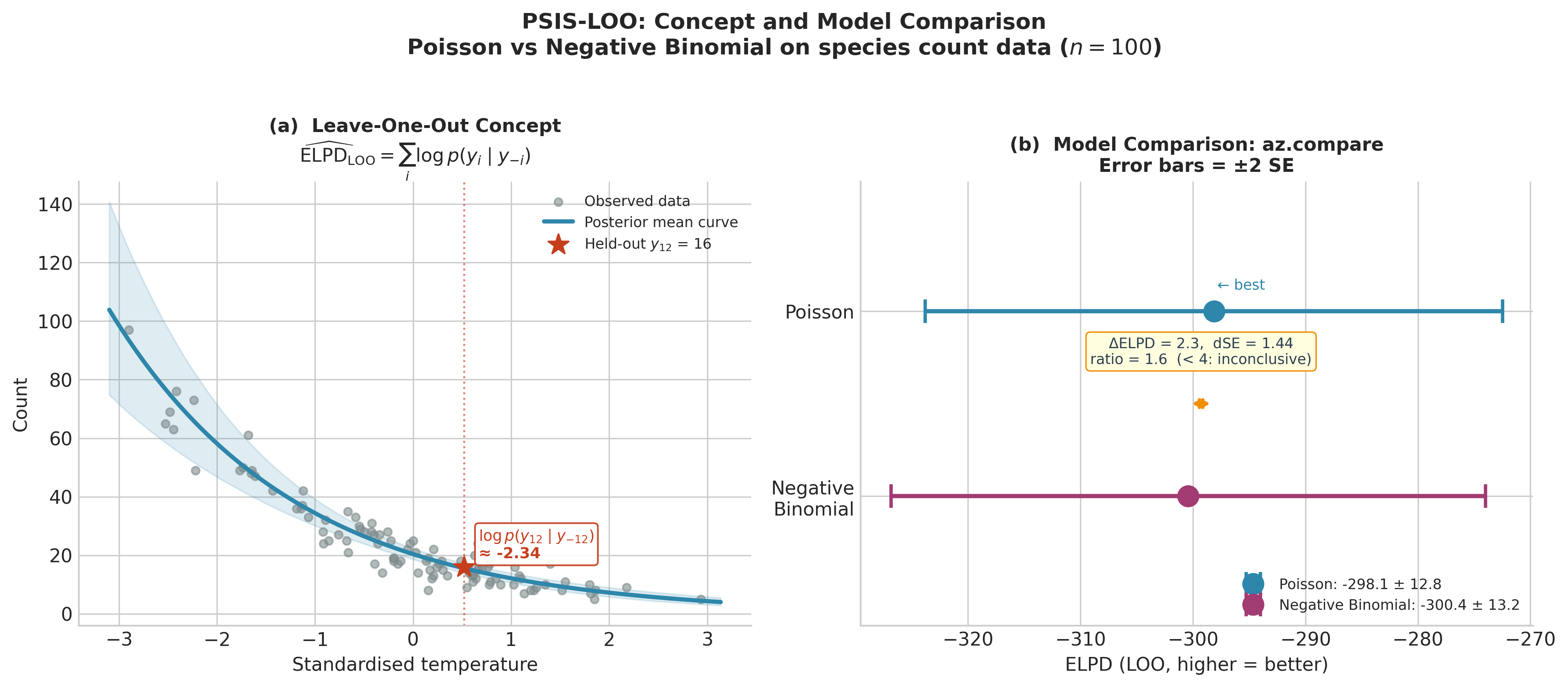
Fig. 221 Figure 5.31. PSIS-LOO in concept and practice. Left: the leave-one-out idea made concrete — observation 12 (\(y_{12} = 16\)) is held out, the model is fitted on the remaining 99 sites, and the log predictive density \(\log p(y_{12} \mid y_{-12}) \approx -2.34\) is evaluated at the held-out value. Summing this quantity over all 100 observations gives \(\widehat{\mathrm{ELPD}}_{\mathrm{LOO}}\). Right: the az.compare result for Poisson vs Negative Binomial regression. Both models have overlapping \(\pm 2\,\mathrm{SE}\) error bars; the \(\Delta\mathrm{ELPD}/\mathrm{dSE}\) ratio is 1.6, well below the 4.0 threshold for a meaningful difference. On data generated from a Poisson process, the extra dispersion parameter of the Negative Binomial earns no predictive return.

Reading the az.compare Table

The az.compare output is the standard reporting format for model comparison in ArviZ:

• rank: Models sorted best (0) to worst; best = highest ELPD.

• elpd_loo: The ELPD estimate. Differences are on the log scale, so a difference of 1 corresponds to the best model assigning roughly \(e^1 \approx 2.7\) times higher predictive density to held-out data on average per observation.

• p_loo: Effective number of parameters. Much larger than the actual parameter count indicates overfitting or high-leverage observations.

• elpd_diff: ELPD of each model minus ELPD of the best model (always 0 for rank 0).

• dse: Standard error of the difference in ELPD between this model and the best model. The difference is meaningful when elpd_diff > 2 * dse.

• warning: True if any Pareto-\(k > 0.7\) were found. Always inspect the Pareto-\(k\) plot when this flag is set.

Common Pitfall ⚠️

Treating a small ELPD difference as decisive. An ELPD difference of 2 with dse = 3 is not evidence that the better model is actually better — it is within sampling noise. The standard error of the difference (dse) is computed from the pointwise LOO values and accounts for the correlation in how the two models perform on the same observations. Only when elpd_diff > 4 * dse is there strong evidence for a meaningful difference in predictive accuracy.

Checking Pareto-\(k\)

Always plot the Pareto-\(k\) values before trusting LOO results:

import matplotlib.pyplot as plt

fig, axes = plt.subplots(1, 2, figsize=(12, 4))
az.plot_khat(loo_pois, ax=axes[0], show_bins=True)
axes[0].set_title("Pareto-k: Poisson")
az.plot_khat(loo_nb, ax=axes[1], show_bins=True)
axes[1].set_title("Pareto-k: Negative Binomial")
plt.tight_layout()

For well-specified models on this dataset, all Pareto-\(k\) values should fall below 0.5. If any exceed 0.7, investigate those observations: they may be outliers, high-leverage points, or evidence of model misspecification.

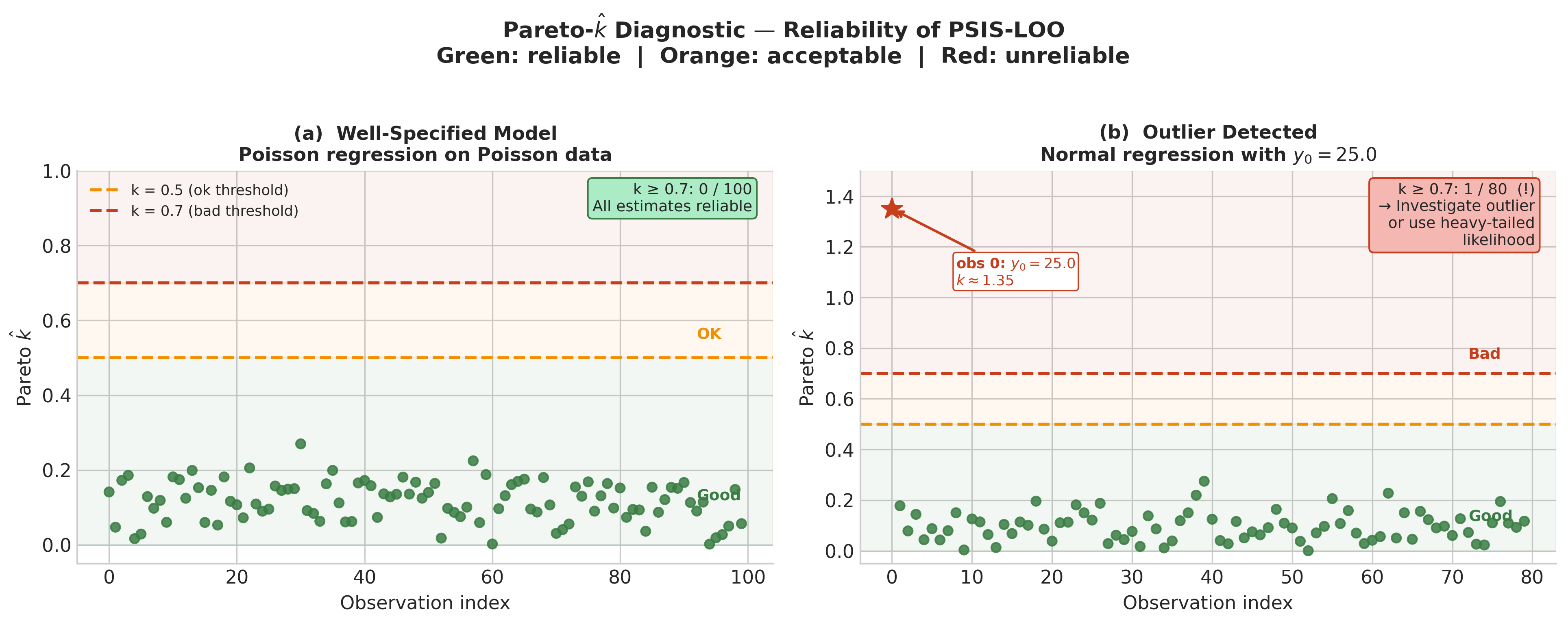
Fig. 222 Figure 5.32. Pareto-\(\hat{k}\) diagnostic: healthy versus problematic LOO. Left: Poisson regression on Poisson-generated data — all 100 Pareto-\(k\) values fall in the good range (\(k < 0.5\), green), confirming that the LOO estimates are reliable for every observation. Right: Normal linear regression with one extreme outlier (\(y_0 = 25.0\), true mean \(\approx 2\)). Observation 0 has \(k \approx 1.35\), far above the bad threshold of 0.7 — the posterior fitted on the full dataset provides almost no information about what the posterior would look like with that observation removed. The guidance box indicates the two standard remedies: investigate the outlier (data error? legitimate extreme event?) or switch to a heavy-tailed likelihood such as Student-\(t\) (Exercise 5.7.2).

Bayes Factors

The Bayes factor for model \(M_1\) over model \(M_2\) is the ratio of their marginal likelihoods:

\[B_{12} = \frac{p(y \mid M_1)}{p(y \mid M_2)}.\]

As established in Section 5.2 Prior Specification and Conjugate Analysis, the marginal likelihood is \(p(y \mid M) = \int p(y \mid \theta, M)\,p(\theta \mid M)\,d\theta\). The Bayes factor has an appealing interpretation: if two models are assigned equal prior probability, then after seeing the data, the posterior odds equal the Bayes factor. A \(B_{12} = 10\) means the data are ten times more probable under \(M_1\) than under \(M_2\).

In practice Bayes factors are rarely used in applied work because:

1. They require proper priors. The marginal likelihood is undefined for improper priors — the very flat priors recommended in Section 5.2 Prior Specification and Conjugate Analysis as weakly informative for regression coefficients are improper. LOO and WAIC do not have this restriction.

2. They are sensitive to prior choice. Unlike ELPD-based methods whose prior sensitivity diminishes as \(n\) grows, the Bayes factor changes substantially with the spread of the prior even for large datasets.

3. They are hard to compute. Estimating the marginal likelihood from MCMC output requires specialised methods (bridge sampling, thermodynamic integration) that are more involved than the log-likelihood sums used by WAIC and LOO.

For conjugate models, the marginal likelihood is available in closed form — the Beta-Binomial expression derived in Section 5.2 Prior Specification and Conjugate Analysis is exactly \(p(y \mid M)\). The idata.log_likelihood computed in §5.6 does not give the marginal likelihood; it gives per-draw pointwise likelihoods, which are the inputs to WAIC and LOO, not to Bayes factors.

The practical recommendation for this course: use LOO for model comparison. Reserve Bayes factors for settings where proper priors can be specified with genuine scientific content and the marginal likelihood can be computed analytically or via bridge sampling.

Bringing It All Together

WAIC and PSIS-LOO both estimate the same target — ELPD — from the same input — the pointwise log-likelihood matrix — and typically agree closely. LOO is preferred because its Pareto-\(k\) diagnostic provides observation-level reliability information that WAIC lacks. The workflow is:

1. Fit competing models in PyMC with idata_kwargs={"log_likelihood": True}.

2. Run az.loo on each model; inspect Pareto-\(k\) via az.plot_khat.

3. Compare with az.compare; read elpd_diff against dse.

4. Treat differences smaller than 4 * dse as inconclusive.

Model comparison answers a different question from the posterior predictive checks in Section 5.6 Probabilistic Programming with PyMC. PPC asks whether one model is self-consistent; LOO asks which of several models predicts better. In a complete Bayesian workflow both are used: PPC first to screen for gross misspecification, LOO to rank adequately-specified alternatives.

The hierarchical models in ch5_8-hierarchical-models provide the most compelling use case for model comparison: should school-level effects be pooled completely (one shared parameter), not at all (separate parameters per school), or partially (hierarchical shrinkage)? LOO quantifies which answer the data support.

Key Takeaways 📝

1. Core concept: ELPD is the predictive accuracy target; both WAIC and PSIS-LOO estimate it from the pointwise log-likelihood matrix without refitting the model. (LO 3)

2. Computational insight: PSIS-LOO is preferred over WAIC because the Pareto-\(k\) diagnostic identifies observations where the LOO estimate is unreliable — WAIC provides no such per-observation reliability check. (LO 4)

3. Practical application: az.compare reports elpd_diff and dse; a difference is meaningful only when elpd_diff > 4 * dse. Bayes factors are theoretically elegant but require proper priors and specialised computation; LOO is the practical default. (LO 3)

4. Outcome alignment: Model comparison closes the Bayesian workflow loop — PPC checks adequacy, LOO ranks alternatives, and ch5_8-hierarchical-models shows the most important use case. (LO 2, 3)

Exercises

Exercise 5.7.1: LOO vs WAIC Agreement

Using the logistic regression from Section 5.6 Probabilistic Programming with PyMC and a null model (intercept only, no predictor):

with pm.Model() as null_model:
    beta_0 = pm.Normal('beta_0', mu=0, sigma=2.5)
    y = pm.Bernoulli('y', p=pm.math.sigmoid(beta_0), observed=y_obs)
    idata_null = pm.sample(draws=2000, tune=1000, chains=4,
                            target_accept=0.90, random_seed=42,
                            idata_kwargs={"log_likelihood": True},
                            progressbar=False)

(a) Compute LOO and WAIC for both models. Do they agree on which model is better?

(b) Examine the ELPD difference relative to its standard error. Is the logistic model decisively better, or is the difference within noise?

(c) Plot az.plot_khat for both models. Do any observations have \(k > 0.7\)?

Solution

(a) LOO and WAIC will agree: the logistic model with the predictor should substantially outperform the null model because the synthetic data were generated with \(\beta_1 = 2.5\) — a strong effect. Both criteria will assign a much higher ELPD to the logistic model.

(b) With \(n = 200\) observations and a true \(\beta_1 = 2.5\), the ELPD difference will be large (typically 20–40 on the log scale) with dse of order 3–5. The ratio elpd_diff / dse will comfortably exceed 4 — decisive evidence.

(c) For well-specified models on this dataset, all Pareto-\(k\) should be below 0.5. Observations near the decision boundary (where \(p \approx 0.5\)) will have the highest \(k\) values but should still be in the good range.

Exercise 5.7.2: Pareto-k and Outliers

Generate data with one extreme outlier:

rng = np.random.default_rng(42)
n = 80
x = rng.normal(0, 1, n)
y_clean = rng.normal(2 + 1.5 * x, 1.0)
y_outlier = y_clean.copy()
y_outlier[0] = 25.0    # extreme outlier

(a) Fit a Normal linear regression to y_outlier using PyMC (prior: pm.Normal on intercept and slope, pm.HalfNormal on sigma). Compute LOO.

(b) Which observations have \(k > 0.5\)? Does observation 0 appear?

(c) Replace the Normal likelihood with a Student-t likelihood (pm.StudentT('y', nu=4, mu=..., sigma=..., observed=y_outlier)). Recompute LOO. How do the Pareto-\(k\) values change? What does this tell you about the heavy-tailed model’s treatment of the outlier?

Solution

(a) and (b) Observation 0 (the outlier at 25.0) will have a very high Pareto-\(k\), likely above 1.0, because the Normal model assigns negligible likelihood to this extreme value and removing it drastically changes the posterior.

(c) Under the Student-t likelihood, observation 0’s \(k\) will drop substantially — often below 0.5 — because the heavy tails assign meaningful probability to extreme values, so removing one outlier has less impact on the posterior. This is the diagnostic signal that a heavy-tailed likelihood is more appropriate for this data.

References

[Watanabe2010]

Watanabe, S. (2010). Asymptotic equivalence of Bayes cross validation and widely applicable information criterion in singular learning theory. Journal of Machine Learning Research, 11, 3571–3594. The original WAIC paper; establishes the \(p_{\mathrm{WAIC}}\) penalty as the variance of the log-likelihood across posterior draws and proves the connection to Bayes cross-validation.

[Vehtari2017]

Vehtari, A., Gelman, A., and Gabry, J. (2017). Practical Bayesian model evaluation using leave-one-out cross-validation and WAIC. Statistics and Computing, 27(5), 1413–1432. The foundational paper for PSIS-LOO; derives the Pareto-\(k\) diagnostic and provides the thresholds used by ArviZ.

[GelmanBDA3ch7]

Gelman, A., Carlin, J. B., Stern, H. S., Dunson, D. B., Vehtari, A., and Rubin, D. B. (2013). Bayesian Data Analysis (3rd ed.), Ch. 7. Chapman and Hall/CRC. Standard treatment of predictive accuracy, information criteria, and Bayes factors at the level appropriate for this course.

[VehtariGabry2020]

Vehtari, A., and Gabry, J. (2020). Bayesian stacking and pseudo-BMA weights for predictive model averaging. Electron. J. Statist., 14(1), 3529–3555. Extends LOO comparison to model averaging via stacking; the az.compare(method='stacking') option implements these weights.