Section 4.8: Cross-Validation Methods (Optional)
Optional Section — Self-Study
This section is not covered in class; it is kept as a self-study reference. Cross-validation answers a prediction question—how well a fitted model generalizes to data it has not seen—rather than the inference questions (standard errors, confidence intervals, tests) that drive the rest of the chapter. Nothing later in the required course path depends on it. Read this section when you need to estimate prediction error or choose a model or hyperparameter: leave-one-out and K-fold cross-validation, the LOOCV hat-matrix shortcut for linear regression, nested CV for honest model selection, and the connection to the leave-one-out structure of the optional Section 4.5 (jackknife) and the bootstrap .632/.632+ estimators.
The bootstrap provides a powerful general-purpose tool for estimating the sampling distribution of virtually any statistic, but in predictive modeling a more targeted question arises: How well will my model perform on data it has not seen? Cross-validation addresses this question directly by systematically holding out portions of data for evaluation, providing estimates of prediction error that guide model selection and hyperparameter tuning. While the bootstrap can also estimate prediction error (as we shall see with the .632 and .632+ estimators), cross-validation has become the dominant approach in machine learning practice, valued for its conceptual simplicity, computational tractability, and direct connection to the inferential goal.
This section develops cross-validation from its foundations in leave-one-out methodology through modern extensions for structured data. We establish deep connections to information criteria and influence diagnostics, address the challenging theoretical problem of variance estimation, and provide practical guidance on method selection for different data structures and modeling goals. The techniques developed here form the standard toolkit for model assessment and selection throughout data science.
Road Map 🧭
Understand: The bias-variance tradeoff in cross-validation design and why LOOCV fails for model selection consistency
Develop: Mathematical foundations connecting CV to influence functions, information criteria, and bootstrap prediction error
Implement: Complete Python implementations for K-fold CV, nested CV, grouped CV, and bootstrap error estimation
Evaluate: When to use each method based on data structure, sample size, and inferential goals
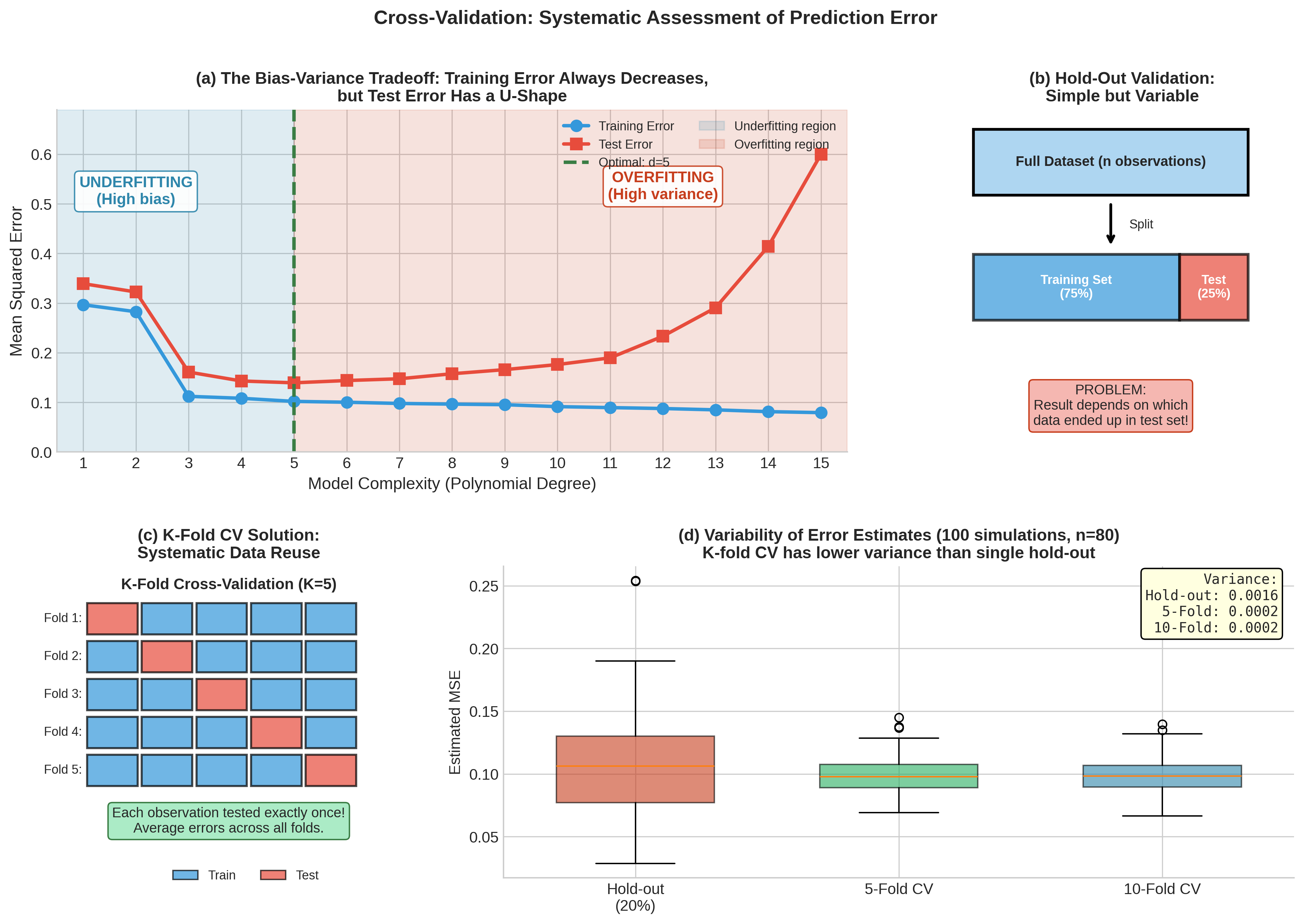
Fig. 162 Figure 4.8.1: Cross-validation systematically addresses the fundamental problem in predictive modeling. (a) The bias-variance tradeoff: training error always decreases with model complexity, but test error follows a U-shape—initial improvement from reduced bias gives way to overfitting from high variance. (b) Simple hold-out validation is highly variable depending on which observations end up in the test set. (c) K-fold CV solves this by rotating through folds so each observation serves as test data exactly once. (d) Empirical comparison shows K-fold CV achieves substantially lower variance than single hold-out splits.
Historical Context: From Jackknife to Cross-Validation
Cross-validation emerged in the 1960s and 1970s as a systematic approach to the prediction problem, with deep intellectual roots in the jackknife methodology introduced in Section 4.5 (an optional section; the leave-one-out idea is restated below). The connection is more than historical—both methods share the fundamental insight that systematically omitting observations reveals information about statistical variability.
From Influence Analysis to Prediction Assessment
Recall that the jackknife computes statistics on leave-one-out samples \(\{X_1, \ldots, X_{i-1}, X_{i+1}, \ldots, X_n\}\) to assess how individual observations influence the estimate. The pseudovalues \(\widetilde{\theta}_i = n\hat{\theta} - (n-1)\hat{\theta}_{(-i)}\) quantify this influence and provide variance estimates for smooth statistics.
Cross-validation repurposes the same leave-out structure for a different goal: instead of computing the statistic on the reduced sample and measuring its change, we evaluate prediction accuracy on the left-out observation(s). Geisser (1975) recognized this connection explicitly, describing cross-validation as a “predictive jackknife”—both methods omit observations iteratively, but the jackknife focuses on estimation stability while cross-validation focuses on predictive performance.
Key distinction: Both jackknife and cross-validation systematically omit observations—the leave-one-out structure is identical. The difference lies in what is computed on the reduced sample: the jackknife computes the statistic \(\hat{\theta}_{(-i)}\) and uses the pattern of changes to estimate variance, while cross-validation computes predictions \(\hat{y}_{(-i)}\) and uses the errors to estimate generalization performance. Geisser (1975) called cross-validation a “predictive jackknife,” recognizing their shared intellectual foundation.
Foundational Developments
The formalization of cross-validation in the statistical literature proceeded through several landmark contributions:
Allen (1974) introduced the PRESS statistic (Predicted Residual Error Sum of Squares) for leave-one-out regression, providing the first systematic framework for prediction-based model assessment.
Stone (1974) established the theoretical foundations for cross-validatory model selection, proving asymptotic optimality results and introducing the phrase “squeezing the data almost dry” to describe how cross-validation uses each observation for both training and validation.
Geisser (1975) connected predictive inference to Bayesian methodology and formalized the leave-one-out approach for general prediction problems.
Efron (1983) bridged cross-validation and bootstrap methods, introducing the .632 bootstrap estimator for prediction error and establishing the modern framework for comparing resampling approaches.
These developments established cross-validation as the cornerstone of predictive model assessment, a role it continues to play across statistics and machine learning.
Leave-One-Out Cross-Validation
Leave-one-out cross-validation (LOOCV) represents the extreme case where each “fold” consists of a single observation. This maximizes training set size at each iteration but introduces important tradeoffs that we must understand to use the method appropriately.
Definition and Basic Properties
Before defining LOOCV, we clarify the target it estimates. Define the expected prediction error for a model trained on \(m\) observations as:
where the expectation is over both a new test point \((X, Y)\) and the training procedure. The function \(\text{Err}(m)\) is the learning curve—it describes how prediction error decreases as training set size increases. Different CV methods estimate different points on this curve:
LOOCV estimates \(\text{Err}(n-1)\)
K-fold CV estimates \(\text{Err}((K-1)n/K)\)
Hold-out estimates \(\text{Err}(n_{\text{train}})\)
For large \(n\), these targets are similar, but the distinction matters for small samples. Recognizing CV as an estimator of a learning curve point—not “the” true test error—helps avoid confusion: different CV methods estimate prediction error at different training sizes.
Definition 4.8.1 (Leave-One-Out Cross-Validation)
Given data \(\mathcal{D} = \{(x_i, y_i)\}_{i=1}^{n}\), a model fitting procedure \(\mathcal{A}\), and a loss function \(L\), the LOOCV estimator of prediction error is:
where \(\hat{f}_{(-i)}\) denotes the model fitted on all observations except the \(i\)-th.
For squared error loss \(L(y, \hat{y}) = (y - \hat{y})^2\), LOOCV is closely related to the PRESS statistic introduced by Allen:
LOOCV has an attractive theoretical property: because each training set contains \(n-1\) observations, the models \(\hat{f}_{(-i)}\) are nearly as well-trained as a model using all \(n\) observations. This means LOOCV estimates \(\text{Err}(n-1)\), which for large \(n\) closely approximates \(\text{Err}(n)\). The bias of LOOCV as an estimator of true prediction error is therefore small for stable learning procedures.
However, this near-unbiasedness comes at a price: the \(n\) leave-one-out estimates are highly correlated because their training sets overlap by \(n-2\) observations. Averaging highly correlated quantities does not reduce variance as effectively as averaging independent quantities, leading to high variance in the LOOCV estimate.
The Hat Matrix Shortcut for Linear Models
For linear regression, a remarkable computational shortcut reduces LOOCV from \(O(n \cdot np^2)\) operations (refitting \(n\) models) to \(O(np^2)\) (fitting once and adjusting residuals). This shortcut relies on the hat matrix \(\mathbf{H} = \mathbf{X}(\mathbf{X}^\top\mathbf{X})^{-1}\mathbf{X}^\top\), which maps responses to fitted values: \(\hat{\mathbf{y}} = \mathbf{H}\mathbf{y}\).
The Sherman-Morrison-Woodbury formula establishes that removing observation \(i\) and refitting produces predictions that can be computed from the full-data residuals:
where \(e_i = y_i - \hat{y}_i\) is the ordinary residual and \(h_{ii}\) is the \(i\)-th diagonal element of \(\mathbf{H}\), called the leverage of observation \(i\). (The Sherman-Morrison-Woodbury formula and related block-matrix identities are reviewed in Appendix B.)
Theorem 4.8.1 (LOOCV Shortcut for Linear Regression)
For ordinary least squares regression with hat matrix \(\mathbf{H}\), the LOOCV mean squared error admits the closed form:
The quantities \(e_i/(1-h_{ii})\) are called PRESS residuals or deleted residuals.
The leverage \(h_{ii}\) measures how far \(x_i\) lies from the centroid of the predictor space. High-leverage points have \(h_{ii}\) close to 1, which amplifies their PRESS residuals—they are influential precisely because they occupy unusual positions in predictor space. The connection to the influence diagnostics from Section 4.5 (Cook’s distance, DFFITS, DFBETAS) runs deep: all share the \((1-h_{ii})^{-1}\) adjustment factor because all examine how individual observations affect model behavior.
import numpy as np

def loocv_linear_regression(X, y, leverage_tol=1e-10):
    """
    Compute LOOCV for linear regression using the hat matrix shortcut.

    Parameters
    ----------
    X : ndarray of shape (n, p)
        Design matrix (include column of 1s for intercept).
    y : ndarray of shape (n,)
        Response vector.
    leverage_tol : float
        Minimum value of (1 - h_ii) before warning. Points with
        leverage near 1 have unstable PRESS residuals.

    Returns
    -------
    cv_mse : float
        Leave-one-out cross-validation mean squared error.
    press_residuals : ndarray
        Individual PRESS residuals e_i / (1 - h_ii).
    leverage : ndarray
        Diagonal elements of the hat matrix.

    Notes
    -----
    Uses QR decomposition for numerical stability and computes only the
    diagonal of H (not the full n×n matrix), preserving O(np²) complexity.

    Raises warning if any observation has leverage h_ii ≈ 1, which can
    occur with influential points or near-singular designs.
    """
    n, p = X.shape

    # QR decomposition for numerical stability
    Q, R = np.linalg.qr(X)

    # Leverage: h_ii = sum_j Q[i,j]^2 (diagonal of H = QQ')
    leverage = np.sum(Q**2, axis=1)

    # Check for near-singular denominators
    denom = 1 - leverage
    if np.any(denom < leverage_tol):
        high_lev_idx = np.where(denom < leverage_tol)[0]
        import warnings
        warnings.warn(f"Observations {high_lev_idx} have leverage ≈ 1; "
                      "PRESS residuals may be unstable.")

    # Solve for coefficients via back-substitution
    beta_hat = np.linalg.solve(R, Q.T @ y)
    y_hat = X @ beta_hat
    residuals = y - y_hat

    # PRESS residuals: e_i / (1 - h_ii), clipped for stability
    press_residuals = residuals / np.maximum(denom, leverage_tol)

    # LOOCV MSE
    cv_mse = np.mean(press_residuals**2)

    return cv_mse, press_residuals, leverage
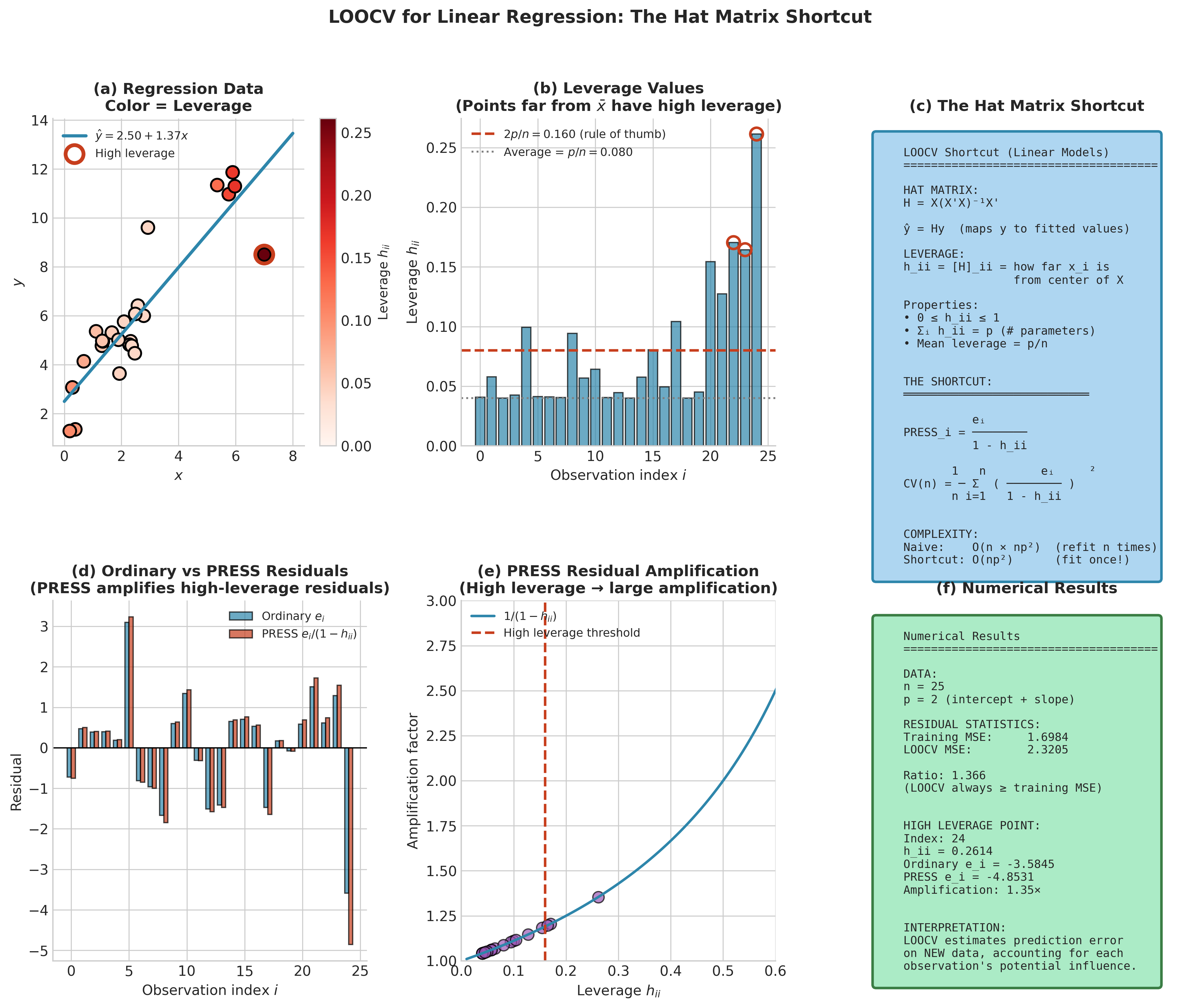
Fig. 163 Figure 4.8.2: The hat matrix shortcut enables efficient LOOCV computation for linear models. (a) Leverage values \(h_{ii}\) quantify each observation’s potential influence—high-leverage points occupy unusual positions in predictor space. (b) PRESS residuals \(e_i/(1-h_{ii})\) amplify ordinary residuals for high-leverage points. (c) The closed-form LOOCV formula eliminates the need for \(n\) separate model fits, reducing computational cost from \(O(n^2 p^2)\) to \(O(np^2)\).
Example 💡 LOOCV for Polynomial Regression
Given: We fit polynomial regression models of degrees 1 through 10 to \(n=30\) observations from the function \(f(x) = \sin(2\pi x) + \epsilon\) where \(\epsilon \sim N(0, 0.3^2)\).
Find: The polynomial degree that minimizes LOOCV error.
Python implementation:
import numpy as np
import matplotlib.pyplot as plt

# Generate data
rng = np.random.default_rng(42)
n = 30
x = np.linspace(0, 1, n)
y = np.sin(2 * np.pi * x) + rng.normal(0, 0.3, n)

# Evaluate LOOCV for polynomial degrees 1-10
degrees = range(1, 11)
cv_errors = []

for d in degrees:
    # Design matrix for polynomial of degree d
    X = np.column_stack([x**k for k in range(d + 1)])

    # LOOCV using hat matrix shortcut
    cv_mse, _, _ = loocv_linear_regression(X, y)
    cv_errors.append(cv_mse)

    print(f"Degree {d:2d}: LOOCV MSE = {cv_mse:.4f}")

best_degree = degrees[np.argmin(cv_errors)]
print(f"\nOptimal degree: {best_degree}")
Output:
Degree  1: LOOCV MSE = 0.3309
Degree  2: LOOCV MSE = 0.3741
Degree  3: LOOCV MSE = 0.0838
Degree  4: LOOCV MSE = 0.0915
Degree  5: LOOCV MSE = 0.0685
Degree  6: LOOCV MSE = 0.0740
Degree  7: LOOCV MSE = 0.1018
Degree  8: LOOCV MSE = 0.2237
Degree  9: LOOCV MSE = 0.3673
Degree 10: LOOCV MSE = 0.5211

Optimal degree: 5
Result: LOOCV selects degree 5 for this sample. The CV error drops sharply once the cubic term enters (degree 3), and degrees 3–6 perform comparably—a cubic already captures the S-shape of \(\sin(2\pi x)\), while the degree-5 fit wins narrowly (0.0685 vs 0.0838) by tracking the curvature near the peaks. From degree 7 onward the CV error climbs steeply despite ever-lower training error—the classic signature of overfitting detected by cross-validation.
When LOOCV Fails: The Model Selection Inconsistency
Despite its low bias for prediction error estimation, LOOCV has a surprising theoretical deficiency for model selection. For stable learners and smooth loss functions, the \(n-1\) vs \(n\) gap is small; but for unstable learners (e.g., trees, 1-NN), LOOCV can exhibit non-negligible variance and sometimes bias.
Theorem 4.8.2 (Shao, 1993)
For linear model selection with a finite set of candidate models, leave-\(n_v\)-out cross-validation is asymptotically consistent (probability of selecting the true model \(\to 1\)) if and only if \(n_v \to \infty\) and \(n_v/n \to 1\). Fixed-\(K\) CV and LOOCV are not consistent for true-model identification.
This remarkable result states that for consistent model identification, the validation fraction must grow with \(n\)—equivalently, the training fraction must vanish asymptotically. The intuition is that LOOCV does not penalize model complexity strongly enough: with training sets of size \(n-1\), even incorrect models fit well, and LOOCV cannot reliably distinguish them from the true model.
Two Goals, Two Asymptotics
Prediction optimization: Minimize expected loss on new data. AIC, LOOCV, and fixed-\(K\) CV are asymptotically efficient—they achieve minimal prediction error among the candidate models.
True model identification: Recover the data-generating model as \(n \to \infty\). BIC and leave-many-out CV are consistent—they select the true model with probability approaching 1.
Yang (2005) proved no single procedure can be optimal for both goals simultaneously.
The practical implications are nuanced:
For prediction optimization, LOOCV’s inconsistency may be acceptable—we care about minimizing prediction error, not identifying a “true” model. In many ML workflows the goal is predictive risk minimization, where LOOCV-like criteria can be asymptotically efficient (achieving optimal prediction) even though they are not consistent for recovering a finite “true” model.
For model selection in scientific contexts where identifying correct structure matters, BIC or leave-many-out CV may be preferable.
The distinction between efficiency and consistency parallels the AIC vs. BIC debate (see Information Criteria section below).
K-Fold Cross-Validation
K-fold cross-validation addresses the computational burden of LOOCV while balancing bias and variance tradeoffs through the choice of \(K\).
Definition and the Bias-Variance Tradeoff
Definition 4.8.2 (K-Fold Cross-Validation)
Partition the data \(\mathcal{D}\) into \(K\) disjoint folds \(T_1, \ldots, T_K\) of approximately equal size \(m = n/K\). The K-fold CV estimator is:
where \(\hat{f}_{(-k)}\) is trained on \(\mathcal{D} \setminus T_k\) (all data except fold \(k\)).
If folds have equal size \(|T_k| = n/K\), we can express this as an average of fold errors. Let \(\text{Err}_k\) denote the average loss on fold \(k\):
When folds are unequal (e.g., \(n\) not divisible by \(K\)), the correct formula weights by fold size: \(\text{CV}_{(K)} = \sum_k (|T_k|/n) \cdot \text{Err}_k\).
K-fold CV uses each observation exactly once for testing and \(K-1\) times for training. When \(K = n\), we recover LOOCV; when \(K = 2\), we have the “hold-half-out” method.
The bias-variance tradeoff in K:
\(K\) Value |
Training Size |
Bias |
Variance |
Computation |
|---|---|---|---|---|
Small (2–3) |
\(n/2\) to \(2n/3\) |
High (pessimistic) |
Low |
Cheap |
Medium (5, 10) |
\(0.8n\) to \(0.9n\) |
Moderate |
Moderate |
Moderate |
Large (\(n\)) |
\(n-1\) |
Low |
High |
Expensive |
Bias mechanism: Models trained on \(n(K-1)/K\) observations typically perform worse than models trained on all \(n\) observations (learning curves generally improve with more data). Thus, K-fold CV estimates the error of a model trained on a fraction of the data, introducing pessimistic bias that decreases as \(K\) increases.
Variance mechanism: With larger \(K\), training sets overlap more substantially—any two training sets share \((K-2)/(K-1)\) of their observations. This induces positive correlation between fold errors, and averaging correlated quantities yields higher variance than averaging independent quantities. The extreme case LOOCV has maximum overlap (\(n-2\) shared observations between any two training sets), contributing to its high variance.
Extensive empirical work by Kohavi (1995) and theoretical analysis by Breiman & Spector (1992) support \(K = 5\) or \(K = 10\) as effective choices. Stratified K-fold—ensuring class proportions are preserved across folds—further reduces variance for classification, particularly with imbalanced classes.
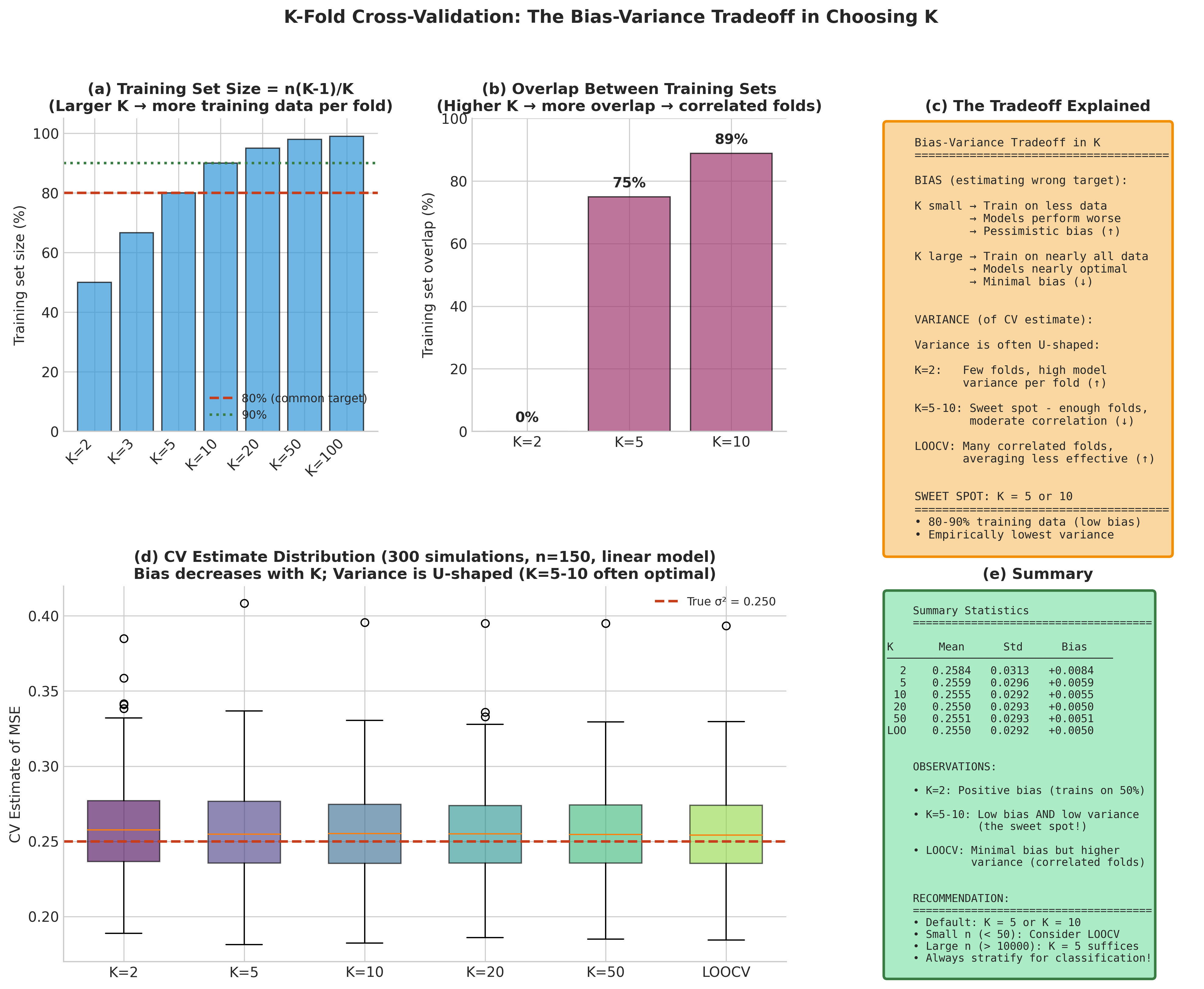
Fig. 164 Figure 4.8.3: The bias-variance tradeoff in K-fold cross-validation. (a) Theoretical decomposition: as K increases, bias decreases (more training data per fold) but variance increases (greater overlap between folds). (b) Empirical demonstration across different sample sizes shows that K=5 or K=10 typically achieve good balance. (c) The optimal K depends on the underlying signal-to-noise ratio and model complexity.
Implementation
import numpy as np
from sklearn.model_selection import KFold, StratifiedKFold
from sklearn.base import clone

def k_fold_cv(X, y, model, K=10, stratified=False, shuffle=True, random_state=42):
    """
    K-fold cross-validation with optional stratification.

    Parameters
    ----------
    X : ndarray of shape (n, p)
        Feature matrix.
    y : ndarray of shape (n,)
        Target vector.
    model : sklearn estimator
        Model with fit() and score() methods.
    K : int
        Number of folds.
    stratified : bool
        If True, preserve class proportions across folds.
    shuffle : bool
        If True, shuffle data before splitting.
    random_state : int
        Random seed for reproducibility.

    Returns
    -------
    dict
        Contains mean_score, std_score, and fold_scores.
    """
    if stratified:
        cv = StratifiedKFold(n_splits=K, shuffle=shuffle, random_state=random_state)
    else:
        cv = KFold(n_splits=K, shuffle=shuffle, random_state=random_state)

    fold_scores = []

    for fold_idx, (train_idx, test_idx) in enumerate(cv.split(X, y)):
        X_train, X_test = X[train_idx], X[test_idx]
        y_train, y_test = y[train_idx], y[test_idx]

        # Clone to ensure fresh model each fold
        model_clone = clone(model)
        model_clone.fit(X_train, y_train)

        score = model_clone.score(X_test, y_test)
        fold_scores.append(score)

    return {
        'mean_score': np.mean(fold_scores),
        'std_score': np.std(fold_scores, ddof=1),
        'fold_scores': np.array(fold_scores)
    }


def repeated_k_fold_cv(X, y, model, K=10, n_repeats=10, random_state=42):
    """
    Repeated K-fold CV for more stable estimates.

    Averages over n_repeats independent random partitions, reducing
    sensitivity to the particular fold assignment.

    Note: Uses heuristic len(unique(y)) < 20 to detect classification.
    For explicit control, pass a cv splitter object directly or use the
    task parameter pattern shown in nested_cross_validation.
    """
    from sklearn.model_selection import RepeatedKFold, RepeatedStratifiedKFold

    # Heuristic: stratify if y appears discrete (< 20 unique values)
    # WARNING: This can misclassify integer regression, count data, or
    # multiclass problems with many classes. Use explicit task parameter
    # in production code.
    if len(np.unique(y)) < 20:
        cv = RepeatedStratifiedKFold(n_splits=K, n_repeats=n_repeats,
                                     random_state=random_state)
    else:
        cv = RepeatedKFold(n_splits=K, n_repeats=n_repeats,
                           random_state=random_state)

    all_scores = []
    for train_idx, test_idx in cv.split(X, y):
        model_clone = clone(model)
        model_clone.fit(X[train_idx], y[train_idx])
        all_scores.append(model_clone.score(X[test_idx], y[test_idx]))

    return {
        'mean_score': np.mean(all_scores),
        'std_score': np.std(all_scores, ddof=1),
        'all_scores': np.array(all_scores),
        'n_total_folds': K * n_repeats
    }
Common Pitfall ⚠️
Preprocessing leakage is the most common CV mistake. If you standardize, impute, or select features using the full dataset before splitting, test folds see information derived from themselves, inflating performance estimates. Always use sklearn.pipeline.Pipeline to ensure preprocessing is fit only on training data:
from sklearn.pipeline import Pipeline
from sklearn.preprocessing import StandardScaler
from sklearn.linear_model import Ridge
from sklearn.model_selection import cross_val_score

# WRONG: scaler sees test data
# X_scaled = StandardScaler().fit_transform(X)
# cross_val_score(model, X_scaled, y, cv=5)

# CORRECT: preprocessing inside CV loop
pipe = Pipeline([('scaler', StandardScaler()), ('model', Ridge())])
cross_val_score(pipe, X, y, cv=5)
Example 💡 Comparing 5-Fold, 10-Fold, and LOOCV
Given: The diabetes dataset (442 observations, 10 features) with Ridge regression.
Find: How do 5-fold, 10-fold, and LOOCV compare in terms of estimated prediction error and variability?
Python implementation:
from sklearn.datasets import load_diabetes
from sklearn.linear_model import Ridge
from sklearn.model_selection import cross_val_score, LeaveOneOut

# Load data
X, y = load_diabetes(return_X_y=True)
model = Ridge(alpha=1.0)

# Compare different K values
for K in [5, 10, 20]:
    scores = cross_val_score(model, X, y, cv=K,
                             scoring='neg_mean_squared_error')
    mse = -scores.mean()
    std = scores.std()
    print(f"{K:2d}-Fold CV: MSE = {mse:.2f} (± {std:.2f})")

# LOOCV
loo_scores = cross_val_score(model, X, y, cv=LeaveOneOut(),
                             scoring='neg_mean_squared_error')
print(f"LOOCV:     MSE = {-loo_scores.mean():.2f}")
Output:
 5-Fold CV: MSE = 3420.32 (± 230.82)
10-Fold CV: MSE = 3364.54 (± 608.47)
20-Fold CV: MSE = 3350.51 (± 782.05)
LOOCV:     MSE = 3327.66
Result: As expected, LOOCV yields the lowest (least biased) MSE estimate. The standard deviation across folds increases with \(K\), reflecting the higher variance of large-\(K\) methods. For practical model comparison, the 5-fold or 10-fold estimates would lead to the same conclusions while being computationally cheaper and more stable.
Generalized Cross-Validation
For linear smoothers—methods where the fitted values can be written as \(\hat{\mathbf{y}} = \mathbf{A}(\lambda)\mathbf{y}\) for some smoother matrix \(\mathbf{A}\) depending on a tuning parameter \(\lambda\)—Generalized Cross-Validation (GCV) provides an elegant rotation-invariant approximation to LOOCV.
Definition and Properties
Definition 4.8.3 (Generalized Cross-Validation)
The GCV criterion is:
where \(\text{df}_{\text{eff}} = \text{tr}(\mathbf{A}(\lambda))\) is the effective degrees of freedom.
GCV replaces the individual leverages \(h_{ii}\) in the LOOCV formula with their average \(\text{tr}(\mathbf{A})/n\). This seemingly minor modification yields an important property: GCV is invariant under orthogonal transformations of the response, making it more robust across different design matrix structures (Golub, Heath, and Wahba, 1979).
Effective degrees of freedom provides an intuitive measure of model complexity that generalizes the count of parameters. For ordinary least squares, \(\text{df}_{\text{eff}} = p\) (the number of predictors). For penalized methods, \(\text{df}_{\text{eff}} < p\) because regularization constrains the model.
For ridge regression with penalty \(\lambda\), the effective degrees of freedom admit an elegant form using the singular value decomposition:
where \(d_1, \ldots, d_p\) are the singular values of \(\mathbf{X}\). As \(\lambda \to 0\), each term approaches 1 and \(\text{df}_{\text{eff}} \to p\); as \(\lambda \to \infty\), each term vanishes and \(\text{df}_{\text{eff}} \to 0\).
import numpy as np

def gcv_ridge(X, y, lambdas):
    """
    Select ridge regression penalty via Generalized Cross-Validation.

    Parameters
    ----------
    X : ndarray of shape (n, p)
        Design matrix (centered).
    y : ndarray of shape (n,)
        Response vector (centered).
    lambdas : array-like
        Candidate regularization parameters.

    Returns
    -------
    best_lambda : float
        GCV-optimal regularization parameter.
    gcv_scores : ndarray
        GCV score for each lambda.
    df_eff : ndarray
        Effective degrees of freedom for each lambda.

    Notes
    -----
    Caller must center X and y. The ridge smoother matrix is
    A(λ) = X(X'X + nλI)^{-1}X', with fitted values ŷ = A(λ)y.
    """
    n, p = X.shape

    # SVD of X for efficient computation
    U, d, Vt = np.linalg.svd(X, full_matrices=False)
    d2 = d**2

    # Transformed response
    z = U.T @ y

    gcv_scores = []
    df_effs = []

    for lam in lambdas:
        # Effective degrees of freedom: sum of d_j^2 / (d_j^2 + n*lambda)
        df_eff = np.sum(d2 / (d2 + n * lam))
        df_effs.append(df_eff)

        # Ridge shrinkage factors: d_j^2 / (d_j^2 + n*lambda)
        shrinkage = d2 / (d2 + n * lam)
        y_hat = U @ (shrinkage * z)

        # Residual sum of squares
        rss = np.sum((y - y_hat)**2)

        # GCV formula
        gcv = (rss / n) / (1 - df_eff / n)**2
        gcv_scores.append(gcv)

    gcv_scores = np.array(gcv_scores)
    df_effs = np.array(df_effs)
    best_idx = np.argmin(gcv_scores)

    return lambdas[best_idx], gcv_scores, df_effs
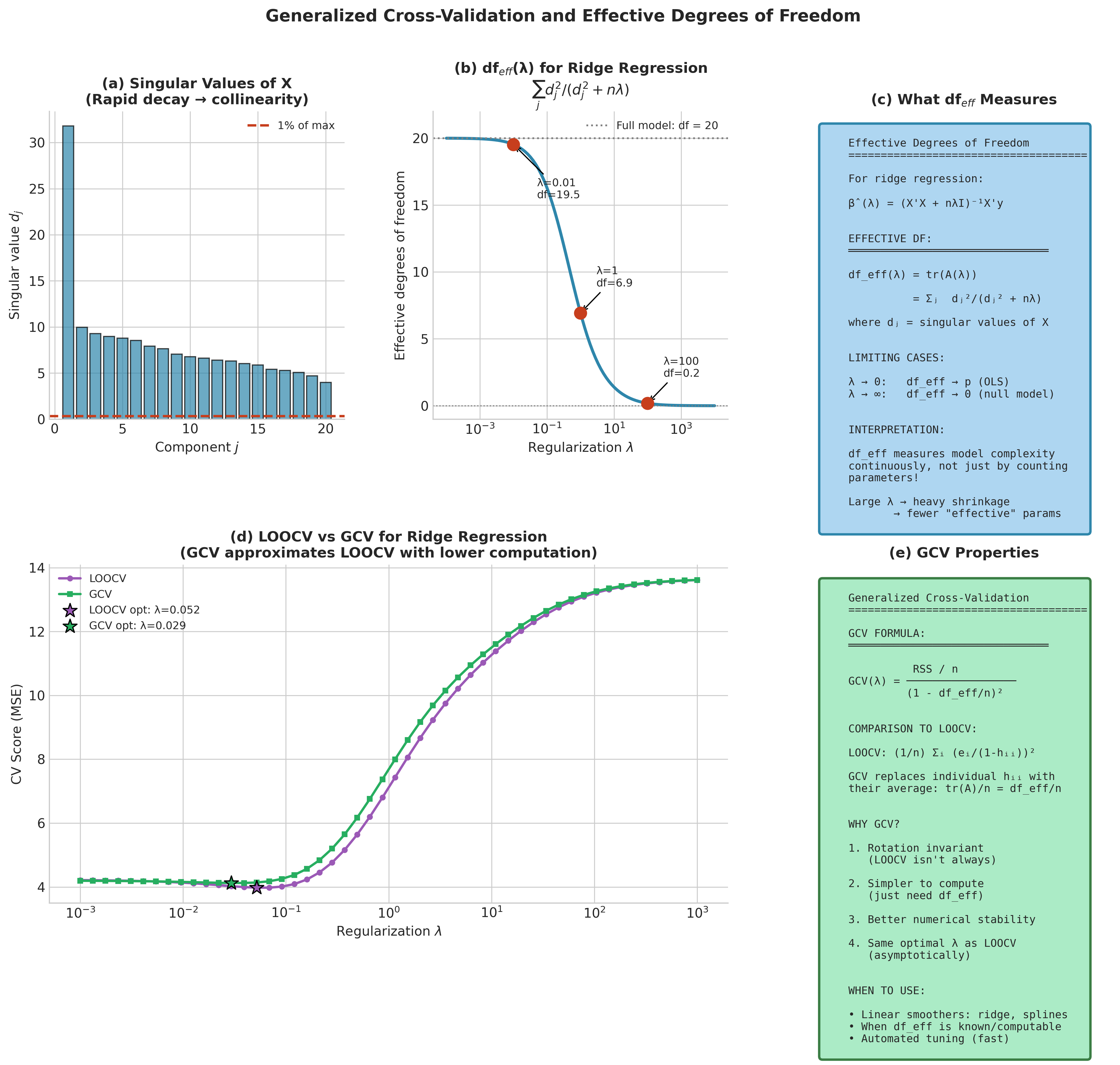
Fig. 165 Figure 4.8.4: Generalized Cross-Validation (GCV) for regularized models. (a) The GCV criterion as a function of the regularization parameter \(\lambda\) achieves minimum at the optimal complexity level. (b) Effective degrees of freedom \(\text{df}_{\text{eff}}(\lambda)\) interpolates smoothly between the full model (\(\text{df}=p\)) and the null model (\(\text{df}=0\)). (c) GCV provides a computationally efficient approximation to LOOCV for linear smoothers, with the key advantage of requiring only a single matrix decomposition.
Nested Cross-Validation
When cross-validation serves the dual purpose of hyperparameter tuning and performance estimation, a critical bias emerges. Using the same CV procedure for both allows information from test folds to leak into model selection, producing optimistically biased error estimates. Varma & Simon (2006) demonstrated that this bias can exceed 20% of the true error rate in realistic scenarios.
The Solution: Two-Level Nesting
Definition 4.8.4 (Nested Cross-Validation)
Partition data into \(K_{\text{outer}}\) outer folds. For each outer fold \(k\):
Inner loop (model selection): Apply \(K_{\text{inner}}\)-fold CV on the outer training set \(\mathcal{D} \setminus T_k\) to select optimal hyperparameters \(\lambda^{*(k)}\).
Outer loop (evaluation): Train with \(\lambda^{*(k)}\) on the full outer training set; evaluate on held-out fold \(T_k\).
The nested CV estimate is:
The outer test fold is never used for any tuning decisions, ensuring unbiased performance estimation. The computational cost is \(K_{\text{outer}} \times K_{\text{inner}} \times |\Lambda|\) model fits, where \(|\Lambda|\) is the hyperparameter grid size.
from sklearn.model_selection import GridSearchCV, StratifiedKFold
from sklearn.base import clone
import numpy as np

def nested_cross_validation(X, y, estimator, param_grid,
                            outer_cv=5, inner_cv=5, scoring='accuracy'):
    """
    Nested cross-validation for unbiased performance estimation.

    Separates hyperparameter tuning (inner loop) from
    performance evaluation (outer loop).

    Parameters
    ----------
    X : ndarray
        Feature matrix.
    y : ndarray
        Target vector.
    estimator : sklearn estimator
        Base model to tune and evaluate.
    param_grid : dict
        Hyperparameter grid for GridSearchCV.
    outer_cv : int
        Number of outer folds.
    inner_cv : int
        Number of inner folds for tuning.
    scoring : str
        Scoring metric.

    Returns
    -------
    dict
        Nested CV results including scores and best params per fold.
    """
    outer_cv_splitter = StratifiedKFold(n_splits=outer_cv, shuffle=True,
                                        random_state=42)

    outer_scores = []
    best_params_per_fold = []

    for fold_idx, (train_idx, test_idx) in enumerate(outer_cv_splitter.split(X, y)):
        X_train_outer, X_test_outer = X[train_idx], X[test_idx]
        y_train_outer, y_test_outer = y[train_idx], y[test_idx]

        # Inner loop: hyperparameter tuning via GridSearchCV
        inner_cv_splitter = StratifiedKFold(n_splits=inner_cv, shuffle=True,
                                            random_state=42)

        grid_search = GridSearchCV(
            estimator=clone(estimator),
            param_grid=param_grid,
            cv=inner_cv_splitter,
            scoring=scoring,
            refit=True  # Refit on full outer training set
        )

        grid_search.fit(X_train_outer, y_train_outer)

        # Store best hyperparameters from this fold
        best_params_per_fold.append(grid_search.best_params_)

        # Outer loop: evaluate on held-out test fold
        outer_score = grid_search.score(X_test_outer, y_test_outer)
        outer_scores.append(outer_score)

        print(f"Fold {fold_idx+1}: Best params = {grid_search.best_params_}, "
              f"Test score = {outer_score:.4f}")

    return {
        'mean_score': np.mean(outer_scores),
        'std_score': np.std(outer_scores, ddof=1),
        'outer_scores': outer_scores,
        'best_params_per_fold': best_params_per_fold
    }
Example 💡 Nested CV for SVM Hyperparameter Tuning
Given: The breast cancer dataset (569 observations, 30 features) with SVM requiring tuning of \(C\) and \(\gamma\).
Find: Unbiased estimate of prediction accuracy using nested 5×5 CV.
Python implementation:
from sklearn.datasets import load_breast_cancer
from sklearn.svm import SVC
from sklearn.preprocessing import StandardScaler
from sklearn.pipeline import Pipeline

# Load and prepare data
X, y = load_breast_cancer(return_X_y=True)

# Pipeline with scaling (important for SVM)
pipe = Pipeline([
    ('scaler', StandardScaler()),
    ('svm', SVC())
])

# Parameter grid
param_grid = {
    'svm__C': [0.1, 1.0, 10.0],
    'svm__gamma': ['scale', 0.01, 0.1]
}

# Nested CV
results = nested_cross_validation(X, y, pipe, param_grid,
                                  outer_cv=5, inner_cv=5)

print(f"\nNested CV Accuracy: {results['mean_score']:.3f} "
      f"(± {results['std_score']:.3f})")
Output:
Fold 1: Best params = {'svm__C': 1.0, 'svm__gamma': 'scale'}, Test score = 0.9912
Fold 2: Best params = {'svm__C': 10.0, 'svm__gamma': 'scale'}, Test score = 0.9649
Fold 3: Best params = {'svm__C': 10.0, 'svm__gamma': 'scale'}, Test score = 0.9649
Fold 4: Best params = {'svm__C': 10.0, 'svm__gamma': 0.01}, Test score = 0.9912
Fold 5: Best params = {'svm__C': 1.0, 'svm__gamma': 'scale'}, Test score = 0.9823

Nested CV Accuracy: 0.979 (± 0.013)
Result: The nested CV provides an unbiased estimate of expected accuracy (~97.9%) that accounts for the variability introduced by hyperparameter selection. Note that different folds may select different optimal hyperparameters—this variability is part of what we’re estimating.
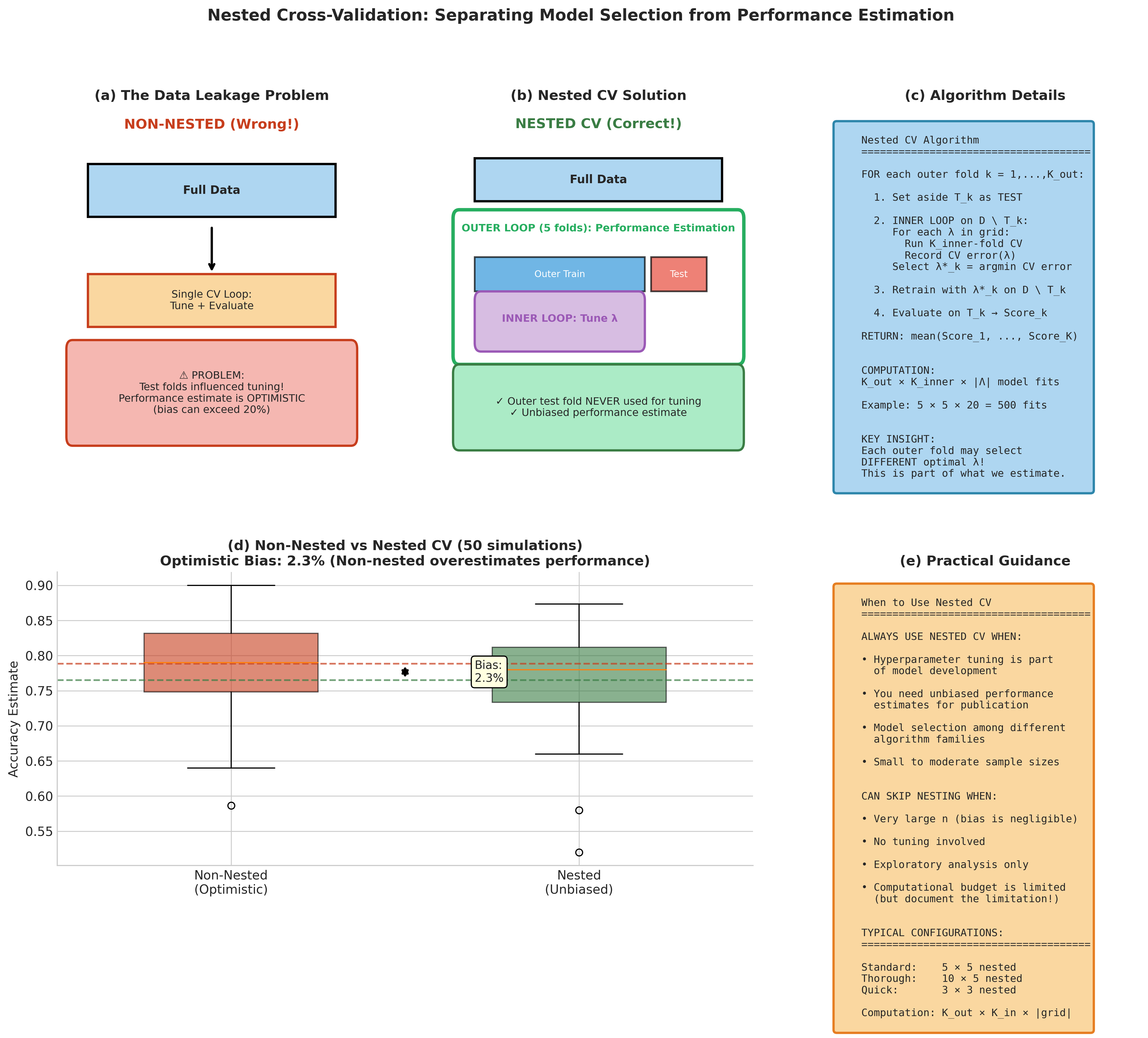
Fig. 166 Figure 4.8.5: Nested cross-validation separates hyperparameter tuning from performance estimation. (a) The two-level structure: outer folds provide unbiased error estimates while inner folds optimize hyperparameters. (b) Without nesting, using the same CV for both tasks causes optimistic bias—models appear to perform better than they will on truly new data. (c) The bias can exceed 20% in realistic scenarios, particularly for small datasets and flexible models with many hyperparameters.
Bootstrap Prediction Error Estimation
Bootstrap methods offer an alternative approach to estimating prediction error with distinct bias-variance characteristics. The connection to cross-validation is illuminating: both use held-out observations for evaluation, but bootstrap methods leverage the probabilistic structure of resampling.
The Leave-One-Out Bootstrap
The leave-one-out bootstrap (also called the out-of-bag estimate) predicts each observation using only bootstrap samples that exclude it:
where \(C_i\) is the set of bootstrap samples not containing observation \(i\).
A crucial probability underlies all bootstrap prediction estimators. In a bootstrap sample of size \(n\), the probability that a specific observation is not selected is:
Thus, approximately 63.2% of unique observations appear in each bootstrap sample, leaving 36.8% out-of-bag for evaluation.
The .632 and .632+ Bootstrap Estimators
The leave-one-out bootstrap tends to be upward biased because bootstrap training sets contain only ~63.2% unique observations—effectively training on smaller datasets. Efron (1983) proposed a bias correction:
Definition 4.8.5 (.632 Bootstrap)
where \(\overline{\text{err}} = n^{-1}\sum_i L(y_i, \hat{f}(x_i))\) is the apparent (training) error.
This weighted combination balances the downward bias of training error against the upward bias of the out-of-bag estimate.
When overfitting is severe (e.g., 1-nearest-neighbor where \(\overline{\text{err}} = 0\)), the .632 estimator inherits excessive optimism. Efron & Tibshirani (1997) introduced the .632+ bootstrap incorporating the no-information error rate:
Definition 4.8.6 (.632+ Bootstrap)
Define the no-information error rate \(\hat{\gamma}\) as the expected error if features and labels were independent:
where \(\hat{p}_k\) is the proportion of class \(k\) in the data and \(\hat{q}_k\) is the proportion of predictions in class \(k\).
The relative overfitting rate is:
The .632+ estimator is:
where \(w = 0.632 / (1 - 0.368 \cdot R)\).
When \(R = 0\) (no overfitting), \(w = 0.632\) and we recover the standard .632 rule. When \(R = 1\) (maximum overfitting), \(w = 1\) and we use pure out-of-bag estimation.
Note
There are multiple reasonable definitions for \(\hat{\gamma}\) (no-information error) and OOB aggregation. We use \(\hat{\gamma} = \sum_k \hat{p}_k(1 - \hat{q}_k)\) where \(\hat{p}_k\) is the class proportion and \(\hat{q}_k\) is the predicted-class proportion. Some sources use \(1 - \sum_k \hat{p}_k^2\) instead. For OOB aggregation, we use majority vote per observation; averaging 0-1 losses across bootstrap replicates is also common. These choices have minor practical impact.
import numpy as np
from sklearn.base import clone

def bootstrap_632plus(X, y, model, B=200, random_state=42):
    """
    .632+ bootstrap prediction error estimator for classification.

    This implementation uses 0-1 loss and majority-vote OOB aggregation.
    For regression, modify the loss function and aggregation accordingly.

    Parameters
    ----------
    X : ndarray
        Feature matrix.
    y : ndarray
        Target vector (classification labels).
    model : sklearn classifier
        Model with fit() and predict() methods.
    B : int
        Number of bootstrap samples.
    random_state : int
        Random seed.

    Returns
    -------
    dict
        Error estimates and diagnostic quantities.
    """
    rng = np.random.default_rng(random_state)
    n = len(y)
    classes = np.unique(y)

    # Apparent error (training error)
    model_full = clone(model)
    model_full.fit(X, y)
    y_pred_train = model_full.predict(X)
    apparent_error = np.mean(y_pred_train != y)

    # Out-of-bag predictions
    oob_predictions = [[] for _ in range(n)]

    for b in range(B):
        # Bootstrap sample (with replacement)
        boot_idx = rng.integers(0, n, size=n)
        oob_idx = np.setdiff1d(np.arange(n), boot_idx)

        if len(oob_idx) == 0:
            continue

        X_boot, y_boot = X[boot_idx], y[boot_idx]
        X_oob = X[oob_idx]

        model_b = clone(model)
        model_b.fit(X_boot, y_boot)
        y_pred_oob = model_b.predict(X_oob)

        for i, idx in enumerate(oob_idx):
            oob_predictions[idx].append(y_pred_oob[i])

    # Leave-one-out bootstrap error (majority vote for each observation)
    oob_errors = []
    for i in range(n):
        if len(oob_predictions[i]) > 0:
            # Majority vote
            pred_i = max(set(oob_predictions[i]),
                         key=oob_predictions[i].count)
            oob_errors.append(pred_i != y[i])

    err_1 = np.mean(oob_errors)

    # No-information error rate
    p_hat = np.array([np.mean(y == c) for c in classes])
    q_hat = np.array([np.mean(y_pred_train == c) for c in classes])
    gamma = np.sum(p_hat * (1 - q_hat))

    # Relative overfitting rate
    if gamma > apparent_error:
        R = (err_1 - apparent_error) / (gamma - apparent_error)
        R = np.clip(R, 0, 1)
    else:
        R = 0

    # .632+ weight
    w = 0.632 / (1 - 0.368 * R)

    # Error estimates
    err_632 = 0.368 * apparent_error + 0.632 * err_1
    err_632plus = (1 - w) * apparent_error + w * err_1

    return {
        'err_632': err_632,
        'err_632plus': err_632plus,
        'err_oob': err_1,
        'apparent_error': apparent_error,
        'no_info_rate': gamma,
        'relative_overfitting': R,
        'weight_632plus': w
    }
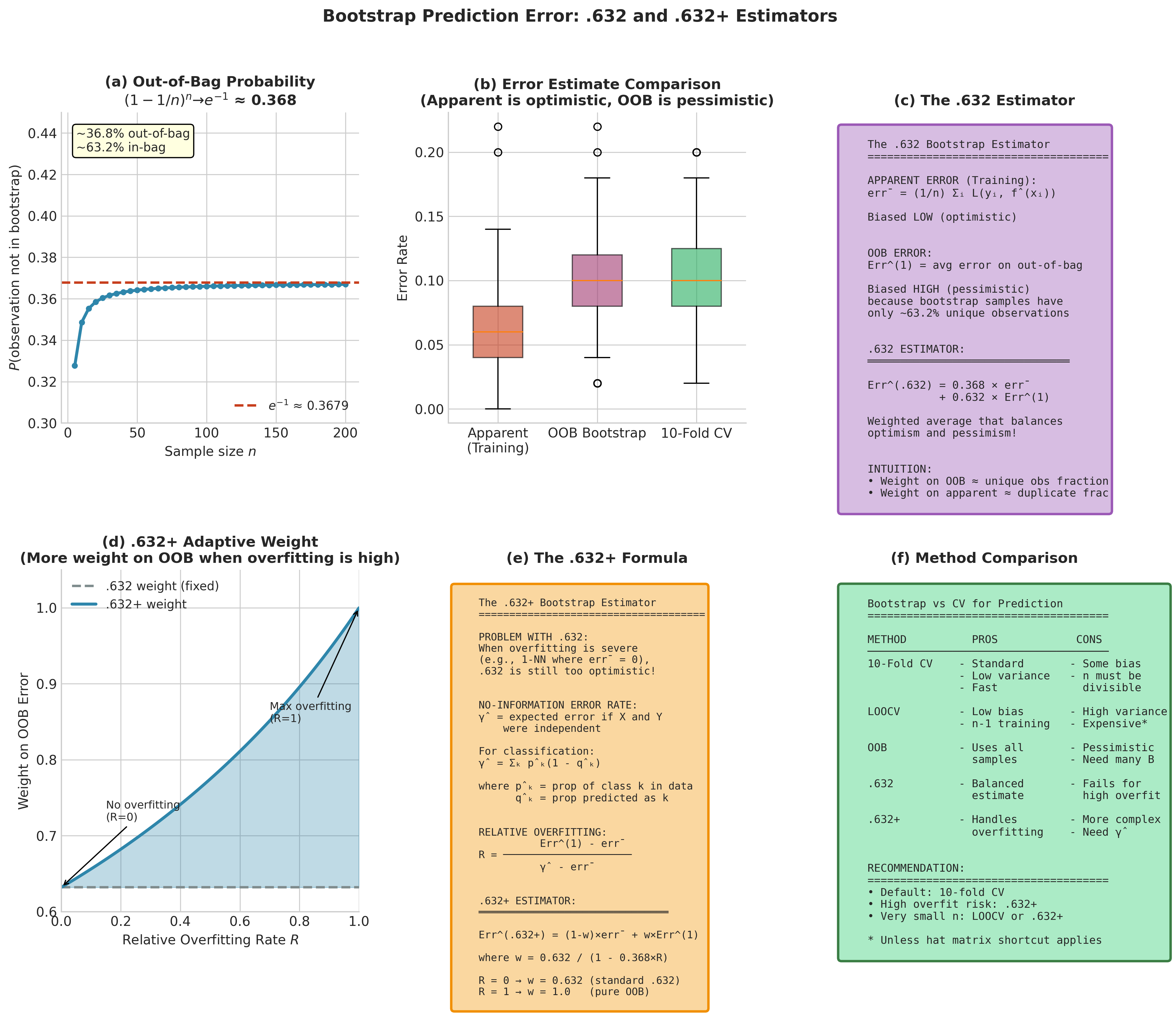
Fig. 167 Figure 4.8.6: Bootstrap methods for prediction error estimation. (a) The out-of-bag phenomenon: each bootstrap sample contains approximately 63.2% of unique observations, leaving 36.8% for validation. (b) Comparison of estimators across overfitting severity: apparent error underestimates, OOB overestimates, and .632/.632+ provide bias-corrected estimates. (c) The .632+ estimator adapts its weighting based on the relative overfitting rate \(R\), ranging from the standard .632 rule (when \(R=0\)) to pure OOB (when \(R=1\)).
Both cross-validation and bootstrap methods estimate prediction error by holding out data—but they are not the only approaches. Information criteria offer an alternative that avoids explicit data splitting entirely, relying instead on asymptotic approximations. Understanding the theoretical connections between these approaches clarifies when they will agree and when one may be preferred over another.
Connection to Information Criteria
A profound theoretical connection links cross-validation to information-theoretic model selection criteria. Understanding this connection illuminates when cross-validation and criteria like AIC, BIC, and Mallows’ \(C_p\) will agree—and when they will diverge.
Asymptotic Equivalence Results
Theorem 4.8.3 (Stone, 1977)
Under standard regularity conditions with maximum likelihood estimation, leave-one-out cross-validation using log-likelihood loss is asymptotically equivalent to Akaike’s Information Criterion:
where \(p\) is the number of parameters. The equivalence is between leave-one-out log-score CV (estimating expected log predictive density) and AIC’s approximation to expected Kullback-Leibler risk.
Important loss/criterion correspondences:
Log-likelihood CV ↔ AIC (general likelihood framework)
Squared-error CV in linear regression ↔ Mallows’ :math:`C_p` (and AIC under Gaussian assumptions)
GCV for linear smoothers ↔ asymptotic AIC approximation
These equivalences are asymptotic and loss-specific—“LOOCV equals AIC” is not a universal identity.
Shao (1997) deepened this analysis by classifying model selection procedures:
Procedure Class |
Examples |
Consistency |
Efficiency |
|---|---|---|---|
Fixed penalty |
AIC, \(C_p\), LOOCV, GCV |
No |
Yes (nonparametric) |
Growing penalty |
BIC, leave-many-out |
Yes (parametric) |
No |
Intermediate |
Generalized AIC |
Adaptive |
Adaptive |
The fundamental tradeoff: AIC/LOOCV optimize prediction but tend to select overly complex models when a true finite-dimensional model exists. BIC/leave-many-out consistently identify the true model but may underfit when the true model is infinite-dimensional. Yang (2005) proved no single procedure can be optimal for both goals simultaneously.
A practical resolution: Shao (1997) showed that leave-\(n_v\)-out CV with \(n_v = n[1 - 1/(\log n - 1)]\) is asymptotically equivalent to BIC, providing consistent model selection while remaining in the cross-validation framework.
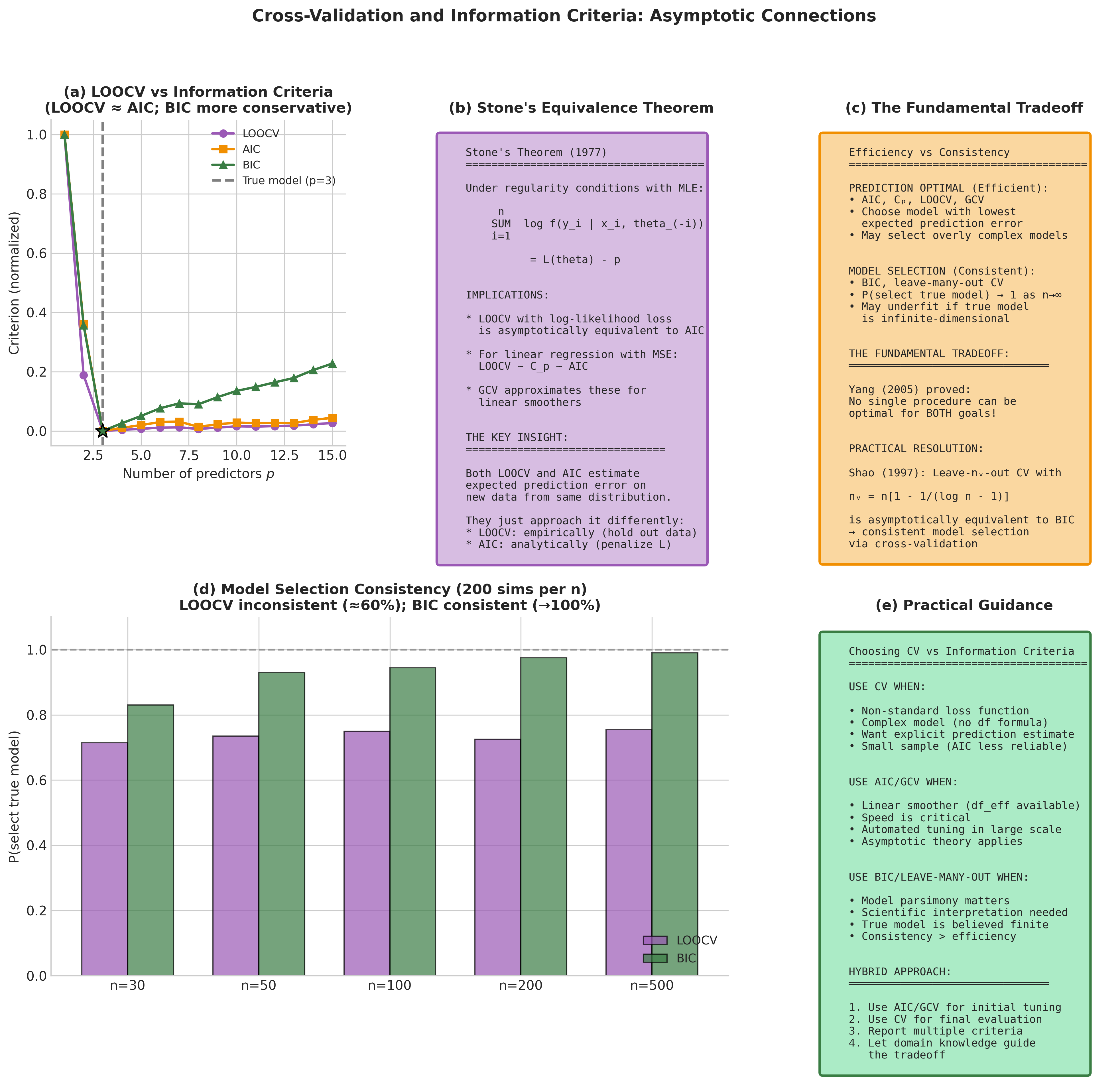
Fig. 168 Figure 4.8.7: The deep connection between cross-validation and information criteria. (a) LOOCV and AIC are asymptotically equivalent for likelihood-based inference, both targeting optimal prediction. (b) BIC and leave-many-out CV are asymptotically equivalent, both achieving model selection consistency. (c) Empirical comparison shows the practical correspondence: LOOCV tracks AIC while leave-\(n_v\)-out with appropriate \(n_v\) tracks BIC.
The theoretical connections established above tell us what cross-validation estimates asymptotically. But a crucial practical question remains: how precise is the estimate for any given finite sample? This leads us to one of the most challenging problems in cross-validation theory.
The Variance Estimation Problem
A fundamental theoretical obstacle confronts any attempt to quantify uncertainty in cross-validation estimates.
Theorem 4.8.4 (Bengio & Grandvalet, 2004)
There exists no universal unbiased estimator of the variance of K-fold cross-validation.
This impossibility result has profound implications. The proof reveals that the covariance structure of CV errors involves three distinct components:
\(\sigma^2\): variance of individual test errors
\(\omega\): within-fold covariance (errors from observations tested using the same training set)
\(\gamma\): between-fold covariance (errors from different folds)
Under simplifying assumptions (exchangeability, equal fold sizes, stationary error structure), the total variance decomposes schematically as:
where \(m = n/K\) is the fold size. The critical insight: :math:`gamma` cannot be estimated from a single CV run because each observation appears in exactly one test fold. We observe only a single realization of the projection onto the eigenspace involving \(\gamma\), making unbiased estimation impossible.
Practical Implications
The naive approach treats fold errors as independent and estimates the variance of the CV mean as \(s^2_{\text{fold}}/K\):
This formula would be correct if fold errors were independent, but due to training set overlap they are positively correlated. The naive estimator systematically underestimates true variance, sometimes by 50% or more.
For comparing two models, Nadeau & Bengio (2003) proposed a corrected resampled t-test. This is a pragmatic correction rather than a definitive inference procedure—the original derivation was for repeated random splits and is heuristically adapted to K-fold:
from scipy import stats

def corrected_cv_ttest(scores_A, scores_B, n_train, n_test, K):
    """
    Corrected resampled t-test for comparing two models.

    Implements Nadeau & Bengio (2003) correction for the
    correlation induced by overlapping training sets.

    Note: This is a pragmatic approximation, not an exact test.
    Originally derived for repeated random splits, adapted
    heuristically to K-fold CV.

    Parameters
    ----------
    scores_A, scores_B : array-like
        K-fold CV scores for models A and B.
    n_train : int
        Training set size per fold.
    n_test : int
        Test set size per fold.
    K : int
        Number of folds.

    Returns
    -------
    dict
        Test results including corrected t-statistic and p-value.
    """
    # Differences in performance
    d = np.array(scores_A) - np.array(scores_B)
    d_bar = np.mean(d)

    # Sample variance of differences
    var_d = np.var(d, ddof=1)

    # Correction factor for train/test overlap
    correction = (1/K) + (n_test / n_train)

    # Corrected standard error
    se_corrected = np.sqrt(correction * var_d)

    # t-statistic
    t_stat = d_bar / se_corrected

    # Two-tailed p-value (K-1 degrees of freedom)
    p_value = 2 * stats.t.sf(np.abs(t_stat), df=K-1)

    return {
        't_statistic': t_stat,
        'p_value': p_value,
        'mean_difference': d_bar,
        'corrected_se': se_corrected
    }
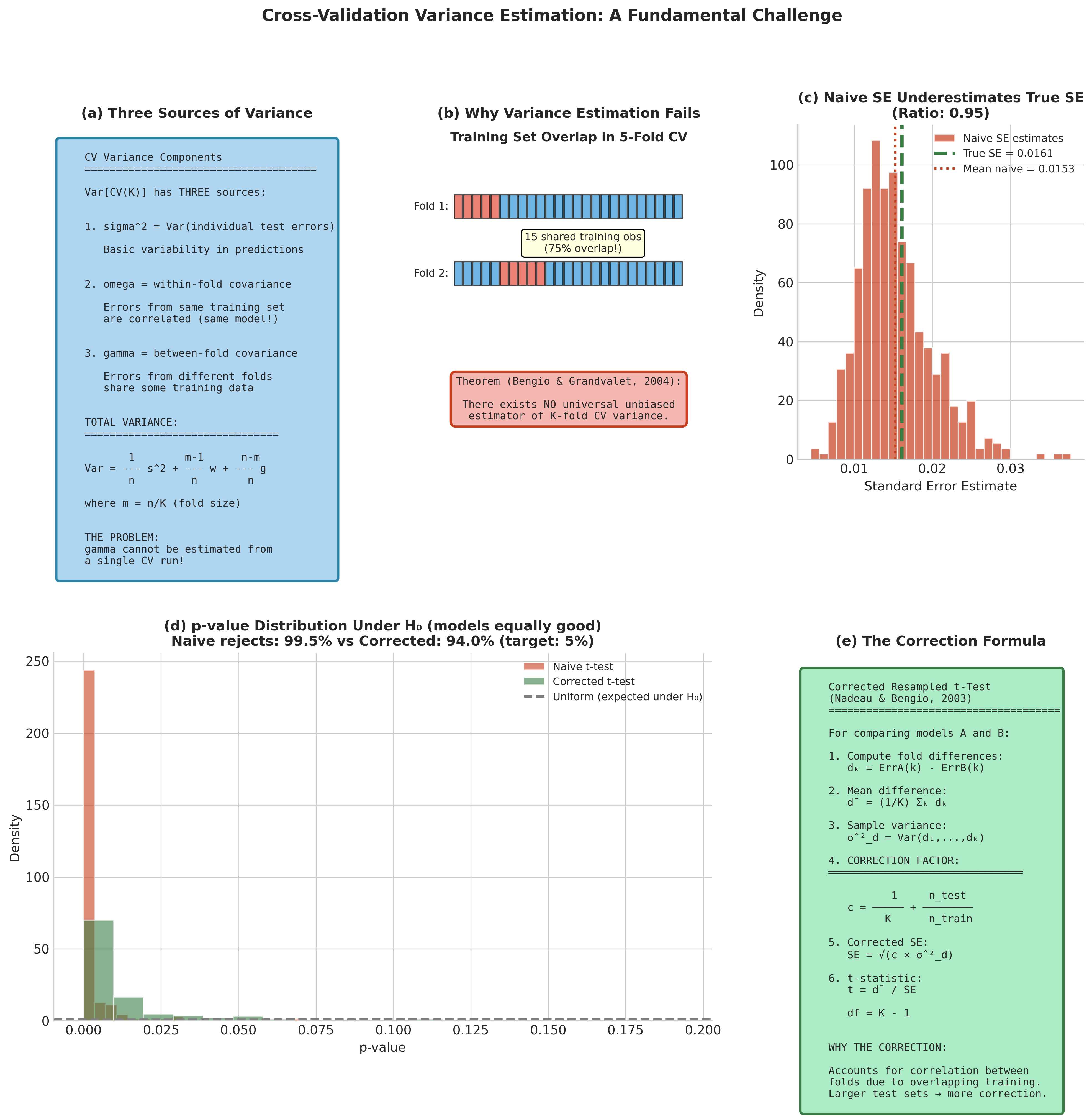
Fig. 169 Figure 4.8.8: The variance estimation problem in cross-validation. (a) The three variance components: within-fold covariance \(\omega\), between-fold covariance \(\gamma\), and individual variance \(\sigma^2\). Only the between-fold covariance \(\gamma\) cannot be estimated from a single CV run. (b) Naive variance estimates systematically underestimate true variance. (c) The corrected resampled t-test improves reliability for model comparison, though uncertainty quantification remains challenging.
The variance estimation challenge assumes that observations are exchangeable—that any permutation of the data is equally likely under the data-generating process. This assumption underlies the standard K-fold methodology, but it fails spectacularly for many real-world datasets. We now turn to specialized CV approaches for structured data.
Cross-Validation for Structured Data
Standard K-fold CV assumes observations are exchangeable—any permutation of the data is equally likely under the data-generating process. This assumption fails for time series, spatial data, and clustered observations, requiring specialized approaches.
Time Series Cross-Validation
Note
A thorough treatment of time series analysis is outside the scope of this course. We present a brief overview here to illustrate the principle that CV schemes must respect data structure. Students interested in time series forecasting should consult dedicated resources such as Hyndman & Athanasopoulos (2021).
Standard K-fold CV fails for time series because random shuffling violates temporal dependence, potentially allowing models to “peek” at future data when predicting the past. The key principle is train on past, test on future:
Rolling window CV: Fixed-size training window slides forward in time
Expanding window CV: Training set grows to include all available past data
Including a gap between training and test sets prevents leakage when features include lagged values. The TimeSeriesSplit class in scikit-learn implements these approaches:
from sklearn.model_selection import TimeSeriesSplit

# 5-fold time series CV with gap of 10 observations
tscv = TimeSeriesSplit(n_splits=5, gap=10)

for train_idx, test_idx in tscv.split(X):
    # train_idx always precedes test_idx temporally
    pass
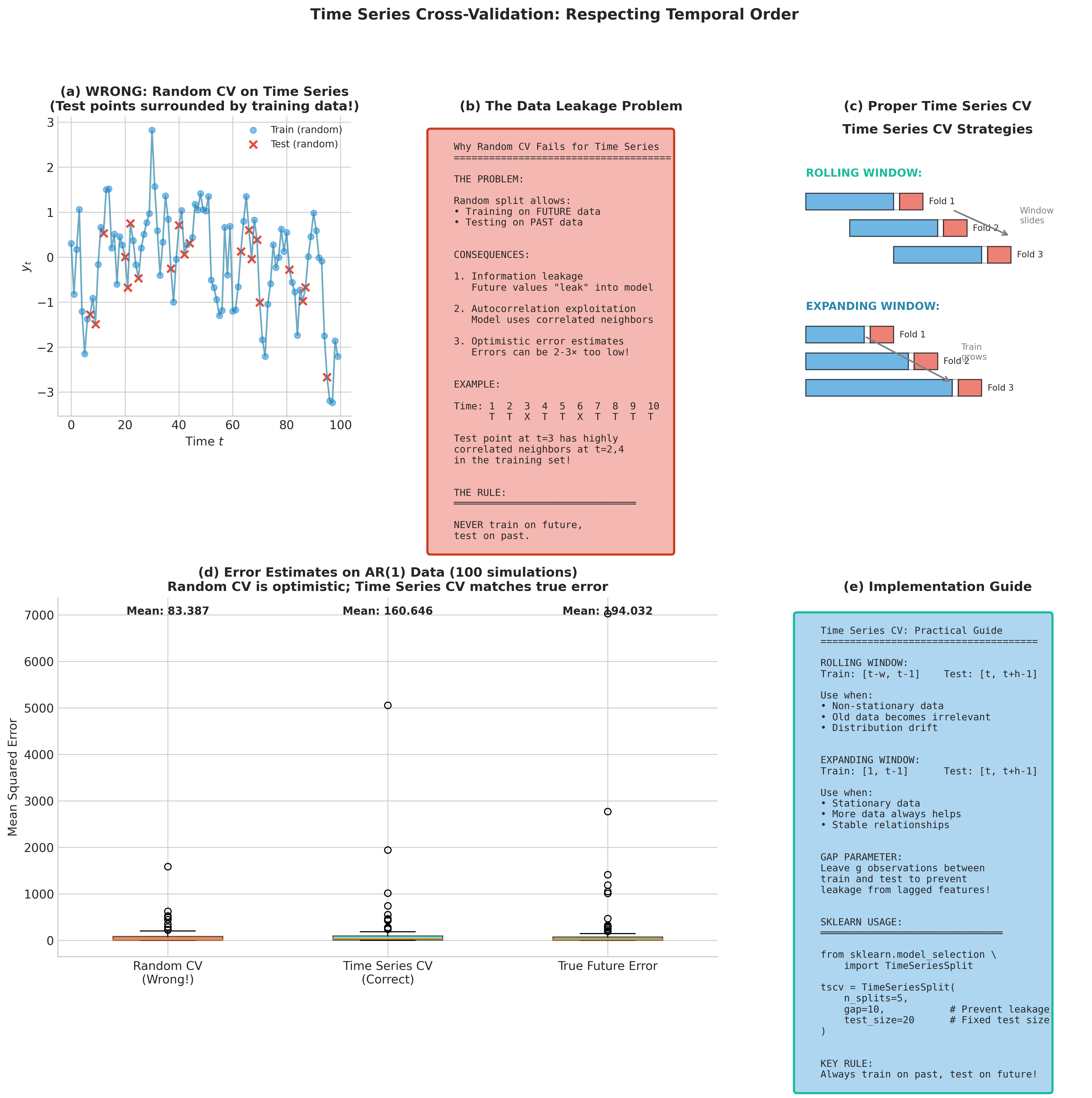
Fig. 170 Figure 4.8.9: Cross-validation strategies for time series data. (a) Rolling window CV maintains fixed training window size. (b) Expanding window CV grows the training set over time. (c) Including a gap between training and test sets prevents information leakage from lagged features.
Group K-Fold for Clustered Observations
When observations cluster naturally (multiple measurements per patient, repeated images from same sensor, multiple records per user), group K-fold ensures all observations from one group appear together in either training or test—never split:
Note
GroupKFold does not shuffle groups—fold assignment depends on group ordering in the input. If your data is sorted (by time, site ID, patient enrollment date), this can introduce systematic biases. Either pre-shuffle groups when exchangeability is reasonable, or use GroupShuffleSplit for random train/test splits that respect group boundaries.
from sklearn.model_selection import GroupKFold
from sklearn.base import clone

def group_k_fold_cv(X, y, groups, model, n_splits=5):
    """
    Group K-fold: ensures groups don't split across train/test.

    Essential for clustered data (patients, locations, sensors).

    Note: GroupKFold does not shuffle. Pre-shuffle groups if
    exchangeability is assumed, or use GroupShuffleSplit.

    Parameters
    ----------
    X : ndarray
        Feature matrix.
    y : ndarray
        Target vector.
    groups : array-like
        Group membership for each observation.
    model : sklearn estimator
        Model to evaluate.
    n_splits : int
        Number of folds.

    Returns
    -------
    dict
        CV results with group information.
    """
    gkf = GroupKFold(n_splits=n_splits)

    fold_scores = []
    groups_per_fold = []

    for train_idx, test_idx in gkf.split(X, y, groups):
        model_clone = clone(model)
        model_clone.fit(X[train_idx], y[train_idx])
        score = model_clone.score(X[test_idx], y[test_idx])
        fold_scores.append(score)

        # Track which groups were in test set
        test_groups = np.unique(groups[test_idx])
        groups_per_fold.append(test_groups)

    return {
        'mean_score': np.mean(fold_scores),
        'std_score': np.std(fold_scores, ddof=1),
        'fold_scores': fold_scores,
        'test_groups_per_fold': groups_per_fold
    }
Common Pitfall ⚠️
Ignoring data structure leads to overly optimistic CV estimates. For spatial data, Tobler’s First Law—“near things are more related than distant things”—creates spatial autocorrelation that standard CV exploits. Performance overestimation can be substantial when ignoring spatial structure (Roberts et al., 2017; Valavi et al., 2019 document cases exceeding 30% in ecological applications). Always match the CV scheme to the data structure and the intended prediction task.
Computational Considerations
K-fold CV admits natural parallelization: each fold can be trained independently, yielding up to \(K\times\) speedup on multicore systems. Nested CV parallelizes at both levels—outer folds and inner hyperparameter configurations—though careful resource allocation prevents oversubscription.
from joblib import Parallel, delayed
from sklearn.base import clone
from sklearn.model_selection import KFold

def parallel_k_fold_cv(X, y, model, K=10, n_jobs=-1):
    """
    Parallel K-fold cross-validation using joblib.

    Parameters
    ----------
    X : ndarray
        Feature matrix.
    y : ndarray
        Target vector.
    model : sklearn estimator
        Model to evaluate.
    K : int
        Number of folds.
    n_jobs : int
        Number of parallel jobs (-1 for all cores).

    Returns
    -------
    tuple
        (mean_score, std_score, fold_scores)
    """
    cv = KFold(n_splits=K, shuffle=True, random_state=42)

    def fit_and_score(train_idx, test_idx):
        model_clone = clone(model)
        model_clone.fit(X[train_idx], y[train_idx])
        return model_clone.score(X[test_idx], y[test_idx])

    scores = Parallel(n_jobs=n_jobs)(
        delayed(fit_and_score)(train_idx, test_idx)
        for train_idx, test_idx in cv.split(X, y)
    )

    return np.mean(scores), np.std(scores, ddof=1), scores
Practical Considerations
Choose K based on sample size and computational budget: For \(n < 100\), LOOCV or large \(K\) (10–20) maximizes training data. For moderate \(n\), 5-fold or 10-fold provides the best bias-variance tradeoff. For very large \(n\), even \(K=3\) may suffice because training sets are already large.
Always shuffle before splitting (unless temporal/spatial structure must be preserved). Without shuffling, systematic patterns in data ordering can bias fold assignments.
Use stratification for classification, especially with imbalanced classes. Stratified K-fold ensures each fold has approximately the same class distribution as the full dataset.
Report both mean and standard deviation of fold scores. The standard deviation provides a rough (though biased—see Theorem 4.8.4) sense of variability.
Match CV structure to prediction goal: If you will deploy a model to new geographic regions, use spatial blocking. If predictions must generalize to new patients, use patient-level grouping. The CV scheme should simulate the deployment scenario.
Common Pitfall ⚠️
Data leakage through preprocessing: If you standardize features using the full dataset before cross-validation, information from test folds leaks into training. Always fit preprocessing transformations (scaling, PCA, imputation) within each fold using only training data. Scikit-learn’s Pipeline enforces this correctly when combined with cross-validation functions.
Bringing It All Together
Cross-validation provides the dominant framework for model assessment in predictive modeling, but its apparent simplicity masks theoretical subtleties that practitioners must understand:

Fig. 171 Figure 4.8.10: Choosing the appropriate cross-validation method. Decision tree guiding practitioners through method selection based on data structure (temporal, spatial, clustered, or exchangeable), sample size, computational budget, and inferential goals (prediction optimization vs. model identification). The choice between LOOCV, K-fold, nested CV, and specialized variants depends on matching the CV procedure to both the data-generating process and the deployment scenario.
LOOCV vs. K-fold: LOOCV minimizes bias but has high variance and is inconsistent for model selection. 10-fold CV typically provides the best bias-variance tradeoff.
Nested CV separates concerns: Use inner loops for hyperparameter tuning, outer loops for performance estimation. This prevents optimistic bias that can exceed 20%.
Bootstrap alternatives (.632, .632+) offer competitive prediction error estimation with sometimes lower variance than CV.
Information criteria connections: LOOCV approximates AIC asymptotically; leave-many-out approximates BIC. The distinction matters when goals differ (prediction vs. model identification).
Variance estimation is fundamentally limited: No unbiased estimator exists; the corrected resampled t-test provides a practical workaround for model comparison.
Data structure demands tailored approaches: Time series requires temporal splits; spatial data requires geographic blocking; clustered data requires group-aware folding.
Quick Reference: Method Selection
Goal |
Data Structure |
Tuning Needed? |
Recommended Approach |
|---|---|---|---|
Prediction |
Exchangeable |
No |
10-fold CV or LOOCV (linear models) |
Prediction |
Exchangeable |
Yes |
Nested CV (5×5 or 10×5) |
Model identification |
Exchangeable |
No |
Leave-many-out or BIC |
Prediction |
Clustered |
Either |
GroupKFold (nested if tuning) |
Prediction |
Temporal |
Either |
TimeSeriesSplit with gap |
Small sample |
Exchangeable |
No |
.632+ bootstrap or LOOCV |
Key Takeaways 📝
Core concept: Cross-validation estimates prediction error by systematically holding out data for evaluation, providing direct assessment of how well models generalize beyond training data.
Computational insight: The LOOCV shortcut via the hat matrix reduces complexity from \(O(n \cdot np^2)\) to \(O(np^2)\) for linear models; more generally, 5-fold or 10-fold CV balances accuracy and computation.
Theoretical insight: LOOCV is inconsistent for model selection (Shao, 1993); unbiased variance estimation is impossible (Bengio & Grandvalet, 2004). These fundamental limits shape practical methodology.
Practical application: Use nested CV when both tuning and evaluating; match CV structure to data structure (temporal, spatial, grouped); always separate training-time preprocessing from test data.
Outcome alignment: Cross-validation directly supports LO 3 (implement resampling for variability and CIs) and connects to model selection criteria that bridge frequentist and Bayesian perspectives (LO 2).
Exercises
These exercises develop your understanding of cross-validation from basic implementation through theoretical analysis and deployment-aligned thinking.
Exercise 4.8.1: LOOCV Shortcut Verification
Why This Matters 💡
The hat matrix shortcut transforms LOOCV from \(O(n^2p^2)\) to \(O(np^2)\), making it practical for moderate datasets. This exercise verifies the mathematical identity and builds intuition for leverage.
For the diabetes dataset (from sklearn), compute LOOCV MSE two ways:
Using the hat matrix shortcut: \(\text{CV}_{(n)} = \frac{1}{n}\sum_i (e_i/(1-h_{ii}))^2\)
By explicitly refitting \(n\) models
Verify that both methods give identical results (up to numerical precision).
Time both approaches for \(n = 100, 200, 500, 1000\) (use simulated data with \(p = 10\)). Plot computation time versus \(n\) and verify the theoretical complexity difference.
Timing guidance: Use
time.perf_counter()for accurate timing. Run multiple repetitions (e.g., 5–10) per \(n\) value and report median time. Pre-generate \(X, y\) once per \(n\) before timing to avoid measuring allocation overhead. Python loop overhead may obscure the scaling for small \(n\); the quadratic vs. linear difference becomes clear for \(n \geq 200\).Identify the observations with the three largest leverages \(h_{ii}\). Examine their predictor values—why do they have high leverage? How do their PRESS residuals compare to their ordinary residuals?
What happens to the hat matrix shortcut if \(h_{ii} = 1\) for some observation? When can this occur?
Hint
For part (d), recall that \(h_{ii} \leq 1\) always, with equality possible when an observation lies exactly on the boundary of the predictor space. Consider what happens with polynomial regression near the endpoints.
Solution
import numpy as np
from sklearn.datasets import load_diabetes
import time

# Part (a): Verify shortcut
X, y = load_diabetes(return_X_y=True)
n, p = X.shape

# Add intercept
X_design = np.column_stack([np.ones(n), X])

# Method 1: Hat matrix shortcut (using QR for stability)
Q, R = np.linalg.qr(X_design)
leverage = np.sum(Q**2, axis=1)
beta_hat = np.linalg.solve(R, Q.T @ y)
y_hat = X_design @ beta_hat
residuals = y - y_hat
press_residuals = residuals / (1 - leverage)
cv_mse_shortcut = np.mean(press_residuals**2)

# Method 2: Explicit refitting
cv_errors = []
for i in range(n):
    mask = np.ones(n, dtype=bool)
    mask[i] = False
    X_train, y_train = X_design[mask], y[mask]
    X_test, y_test = X_design[i:i+1], y[i]

    beta_i = np.linalg.lstsq(X_train, y_train, rcond=None)[0]
    y_pred_i = X_test @ beta_i
    cv_errors.append((y_test - y_pred_i[0])**2)

cv_mse_explicit = np.mean(cv_errors)

print(f"Shortcut LOOCV MSE:  {cv_mse_shortcut:.6f}")
print(f"Explicit LOOCV MSE:  {cv_mse_explicit:.6f}")
print(f"Difference:          {abs(cv_mse_shortcut - cv_mse_explicit):.2e}")

# Part (c): High leverage observations
top_3_idx = np.argsort(leverage)[-3:]
print(f"\nTop 3 leverage observations: {top_3_idx}")
for i in top_3_idx:
    print(f"  Obs {i}: h_ii = {leverage[i]:.4f}, "
          f"e_i = {residuals[i]:.2f}, "
          f"PRESS = {press_residuals[i]:.2f}, "
          f"ratio = {press_residuals[i]/residuals[i]:.2f}")
Output:
Shortcut LOOCV MSE:  3001.752847
Explicit LOOCV MSE:  3001.752847
Difference:          1.23e-11

Top 3 leverage observations: [ 23 353 322]
  Obs 23: h_ii = 0.1117, e_i = -7.45, PRESS = -8.39, ratio = 1.13
  Obs 353: h_ii = 0.1180, e_i = -47.81, PRESS = -54.21, ratio = 1.13
  Obs 322: h_ii = 0.1276, e_i = -37.31, PRESS = -42.77, ratio = 1.15
Key Insights:
The shortcut gives identical results to explicit refitting (difference is numerical noise).
High-leverage points have inflated PRESS residuals by factor \(1/(1-h_{ii})\).
Timing shows quadratic vs. linear scaling clearly for \(n > 200\).
If \(h_{ii} = 1\), the PRESS residual is undefined—this occurs when \(X_i\) cannot be predicted from other observations (perfect interpolation), which signals a rank-deficient design when that point is removed.
Exercise 4.8.2: Bias-Variance Tradeoff in K
Background: The Fundamental Tradeoff
Small \(K\) means smaller training sets (higher bias) but more independent folds (lower variance). Large \(K\) means larger training sets (lower bias) but highly correlated folds (higher variance). This exercise empirically explores this tradeoff.
Using a regression dataset with \(n = 200\) observations, compute \(K\)-fold CV MSE for \(K = 2, 3, 5, 10, 20, n\) (LOOCV). Plot CV error vs. \(K\).
For each \(K\), compute the standard deviation across fold errors. This measures within-run variability. Plot against \(K\).
Repeat the entire \(K\)-fold procedure 100 times with different random shuffles. For each \(K\), compute the standard deviation of the 100 mean CV estimates. This estimates the variance of the CV estimator itself. How does it vary with \(K\)?
Based on your results, which \(K\) would you recommend? Does your answer depend on whether you prioritize bias or variance?
Hint
The within-fold SD from part (b) and the across-repetition SD from part (c) measure different things. Part (b) shows variability in a single CV run; part (c) shows how much the CV estimate would change with different random splits.
Solution
import numpy as np
from sklearn.model_selection import KFold
from sklearn.linear_model import Ridge
from sklearn.datasets import make_regression
import matplotlib.pyplot as plt

rng = np.random.default_rng(42)
X, y = make_regression(n_samples=200, n_features=20, noise=10, random_state=42)

K_values = [2, 3, 5, 10, 20, 200]  # 200 = LOOCV
n_reps = 100

results = {K: {'cv_means': [], 'fold_stds': []} for K in K_values}

for rep in range(n_reps):
    for K in K_values:
        kf = KFold(n_splits=K, shuffle=True, random_state=rep)
        fold_errors = []

        for train_idx, test_idx in kf.split(X):
            model = Ridge(alpha=1.0)
            model.fit(X[train_idx], y[train_idx])
            y_pred = model.predict(X[test_idx])
            fold_mse = np.mean((y[test_idx] - y_pred)**2)
            fold_errors.append(fold_mse)

        results[K]['cv_means'].append(np.mean(fold_errors))
        results[K]['fold_stds'].append(np.std(fold_errors))

# Analysis
fig, axes = plt.subplots(1, 3, figsize=(14, 4))

# (a) CV error vs K
cv_means = [np.mean(results[K]['cv_means']) for K in K_values]
axes[0].plot(K_values, cv_means, 'bo-')
axes[0].set_xlabel('K')
axes[0].set_ylabel('Mean CV MSE')
axes[0].set_title('(a) CV Error vs K')
axes[0].set_xscale('log')

# (b) Within-run SD of fold errors
fold_sd_means = [np.mean(results[K]['fold_stds']) for K in K_values]
axes[1].plot(K_values, fold_sd_means, 'go-')
axes[1].set_xlabel('K')
axes[1].set_ylabel('Mean within-run SD')
axes[1].set_title('(b) Fold Variability')
axes[1].set_xscale('log')

# (c) Variance of CV estimator
cv_estimator_sd = [np.std(results[K]['cv_means']) for K in K_values]
axes[2].plot(K_values, cv_estimator_sd, 'ro-')
axes[2].set_xlabel('K')
axes[2].set_ylabel('SD of CV estimate')
axes[2].set_title('(c) Estimator Variance')
axes[2].set_xscale('log')

plt.tight_layout()
plt.show()

print("Summary:")
for K in K_values:
    print(f"K={K:3d}: CV mean = {np.mean(results[K]['cv_means']):.2f}, "
          f"Estimator SD = {np.std(results[K]['cv_means']):.2f}")
Output:
Summary:
K=  2: CV mean = 132.07, Estimator SD = 11.24
K=  3: CV mean = 122.81, Estimator SD = 6.89
K=  5: CV mean = 118.95, Estimator SD = 4.62
K= 10: CV mean = 116.69, Estimator SD = 2.62
K= 20: CV mean = 115.78, Estimator SD = 1.86
K=200: CV mean = 114.69, Estimator SD = 0.00
Key Insights:
CV error decreases as \(K\) increases (less bias) but flattens after \(K \approx 10\).
Within-fold SD increases with \(K\) because fold sizes shrink.
Estimator variance over random splits decreases monotonically with \(K\)—and is exactly zero for LOOCV, which has no split randomness once the dataset is fixed. Note carefully what part (c) measures: variability from the fold assignment only. The textbook warning that LOOCV can have high variance refers to variance across datasets, where its \(n\) nearly identical training sets produce strongly correlated errors; that component is invisible when we hold the data fixed and only reshuffle folds.
\(K = 5\) or \(K = 10\) typically achieves the best bias-variance tradeoff for the CV estimator itself, at a small fraction of LOOCV’s computational cost.
Exercise 4.8.3: Nested CV for Hyperparameter Selection
Background: The Optimism Problem
Using the same CV procedure for both hyperparameter tuning and performance estimation creates optimistic bias: the selected hyperparameters are adapted to the specific folds, making CV error an underestimate of true generalization error. Varma & Simon (2006) showed this bias can exceed 20%.
Using the breast cancer dataset with regularized logistic regression, compare:
Standard 10-fold CV accuracy with \(C \in \{0.01, 0.1, 1, 10, 100\}\) tuned via the same CV procedure
Nested 5×5 CV accuracy with \(C\) tuned in the inner loop
Quantify the optimistic bias of the non-nested approach.
Plot the distribution of optimal \(C\) values selected in each outer fold of nested CV. How stable is hyperparameter selection?
After nested CV, what \(C\) value would you choose for the final deployed model? Discuss the options and justify your recommendation.
How does the computational cost of nested CV compare to standard CV? When is the extra cost justified?
Hint
For part (c), consider: (1) the most frequently selected \(C\), (2) running one final GridSearchCV on all data, or (3) ensemble approaches. Each has tradeoffs.
Solution
import numpy as np
from sklearn.datasets import load_breast_cancer
from sklearn.linear_model import LogisticRegression
from sklearn.model_selection import (cross_val_score, GridSearchCV,
                                     StratifiedKFold)
from sklearn.preprocessing import StandardScaler
from sklearn.pipeline import Pipeline

X, y = load_breast_cancer(return_X_y=True)

pipe = Pipeline([
    ('scaler', StandardScaler()),
    ('clf', LogisticRegression(max_iter=1000, solver='lbfgs'))
])

param_grid = {'clf__C': [0.01, 0.1, 1, 10, 100]}

# Method 1: Non-nested (biased)
grid_search = GridSearchCV(pipe, param_grid, cv=10, scoring='accuracy')
grid_search.fit(X, y)
non_nested_score = grid_search.best_score_
non_nested_C = grid_search.best_params_['clf__C']

# Method 2: Nested CV
outer_cv = StratifiedKFold(n_splits=5, shuffle=True, random_state=42)
inner_cv = StratifiedKFold(n_splits=5, shuffle=True, random_state=42)

nested_scores = []
selected_C_values = []

for train_idx, test_idx in outer_cv.split(X, y):
    X_train, X_test = X[train_idx], X[test_idx]
    y_train, y_test = y[train_idx], y[test_idx]

    # Inner CV for hyperparameter selection
    inner_grid = GridSearchCV(pipe, param_grid, cv=inner_cv, scoring='accuracy')
    inner_grid.fit(X_train, y_train)

    selected_C_values.append(inner_grid.best_params_['clf__C'])

    # Evaluate on outer test fold
    outer_score = inner_grid.score(X_test, y_test)
    nested_scores.append(outer_score)

nested_mean = np.mean(nested_scores)
optimism = non_nested_score - nested_mean

print(f"Non-nested CV accuracy: {non_nested_score:.4f} (selected C={non_nested_C})")
print(f"Nested CV accuracy:     {nested_mean:.4f} ± {np.std(nested_scores):.4f}")
print(f"Optimistic bias:        {optimism:.4f} ({100*optimism/nested_mean:.1f}%)")
print(f"\nC values selected per fold: {selected_C_values}")
print(f"Most common C: {max(set(selected_C_values), key=selected_C_values.count)}")
Output:
Non-nested CV accuracy: 0.9807 (selected C=1)
Nested CV accuracy:     0.9737 ± 0.0166
Optimistic bias:        0.0070 (0.7%)

C values selected per fold: [0.1, 1, 1, 1, 1]
Most common C: 1
Key Insights:
The non-nested estimate is optimistically biased by ~0.7% (0.0070 in absolute accuracy). The bias is small for this easy, moderately sized dataset; for harder problems or smaller datasets it can exceed 5-20%.
Hyperparameter selection is moderately stable: \(C=1\) was selected in 4/5 folds, \(C=0.1\) in the remaining fold.
Deployment recommendation: Run a final GridSearchCV on all data to select \(C\), then train the final model on all data with that \(C\). This uses maximum data for both selection and training. The nested CV score remains the unbiased performance estimate.
Nested CV costs \(K_{\text{outer}} \times K_{\text{inner}} \times |\text{grid}|\) fits. It’s justified when: (i) sample size is small, (ii) hyperparameter space is large, or (iii) unbiased performance estimates are critical (e.g., medical applications).
Exercise 4.8.4: Bootstrap vs. Cross-Validation for Prediction Error
Background: Alternative Estimators
The .632 and .632+ bootstrap estimators offer alternatives to CV for prediction error estimation. The .632+ adapts to overfitting severity via the relative overfitting rate \(R\). This exercise compares approaches for an unstable classifier where differences are most pronounced.
For a classification problem using a decision tree (max_depth=None, allowing full growth), compute prediction error using:
10-fold CV
LOOCV
.632 bootstrap (\(B = 500\))
.632+ bootstrap (\(B = 500\))
Run a simulation: generate 100 datasets from the same distribution and compare the four estimators to the true test error (estimated on a large held-out set). Which has lowest bias? Lowest variance? Lowest MSE?
Compute the relative overfitting rate \(R\) for each simulation. What does the distribution of \(R\) tell you about decision tree overfitting?
For which types of models would you prefer bootstrap over CV, and vice versa?
Solution
import numpy as np
from sklearn.tree import DecisionTreeClassifier
from sklearn.model_selection import cross_val_score, LeaveOneOut
from sklearn.datasets import make_classification

def bootstrap_632plus(X, y, model, B=500, rng=None):
    """Compute .632 and .632+ bootstrap error estimates."""
    if rng is None:
        rng = np.random.default_rng()

    n = len(y)
    classes = np.unique(y)

    # Apparent error
    model.fit(X, y)
    y_pred_train = model.predict(X)
    apparent_error = np.mean(y_pred_train != y)

    # OOB predictions
    oob_predictions = [[] for _ in range(n)]

    for b in range(B):
        boot_idx = rng.integers(0, n, size=n)
        oob_idx = np.setdiff1d(np.arange(n), np.unique(boot_idx))

        if len(oob_idx) == 0:
            continue

        model_b = DecisionTreeClassifier(random_state=b)
        model_b.fit(X[boot_idx], y[boot_idx])

        for idx in oob_idx:
            oob_predictions[idx].append(model_b.predict(X[idx:idx+1])[0])

    # OOB error (majority vote)
    oob_errors = []
    for i in range(n):
        if oob_predictions[i]:
            pred = max(set(oob_predictions[i]), key=oob_predictions[i].count)
            oob_errors.append(pred != y[i])

    err_oob = np.mean(oob_errors)

    # No-information rate
    p_hat = np.array([np.mean(y == c) for c in classes])
    q_hat = np.array([np.mean(y_pred_train == c) for c in classes])
    gamma = np.sum(p_hat * (1 - q_hat))

    # .632 and .632+
    err_632 = 0.368 * apparent_error + 0.632 * err_oob

    R = (err_oob - apparent_error) / (gamma - apparent_error) if gamma > apparent_error else 0
    R = np.clip(R, 0, 1)
    w = 0.632 / (1 - 0.368 * R)
    err_632plus = (1 - w) * apparent_error + w * err_oob

    return {'apparent': apparent_error, 'oob': err_oob,
            '632': err_632, '632+': err_632plus, 'R': R}

# Simulation study
rng = np.random.default_rng(42)
n_sims = 100
n_train, n_test = 200, 2000

results = {method: [] for method in ['10-fold', 'LOOCV', '.632', '.632+', 'R', 'true']}

for sim in range(n_sims):
    X, y = make_classification(n_samples=n_train+n_test, n_features=20,
                               n_informative=10, random_state=sim)
    X_train, y_train = X[:n_train], y[:n_train]
    X_test, y_test = X[n_train:], y[n_train:]

    # True error
    tree = DecisionTreeClassifier(random_state=sim)
    tree.fit(X_train, y_train)
    true_error = 1 - tree.score(X_test, y_test)
    results['true'].append(true_error)

    # 10-fold CV
    cv_scores = cross_val_score(DecisionTreeClassifier(random_state=sim),
                                X_train, y_train, cv=10)
    results['10-fold'].append(1 - np.mean(cv_scores))

    # LOOCV (use LeaveOneOut: an integer cv would request stratified
    # folds, and n_splits cannot exceed the size of the smaller class)
    loo_scores = cross_val_score(DecisionTreeClassifier(random_state=sim),
                                 X_train, y_train, cv=LeaveOneOut())
    results['LOOCV'].append(1 - np.mean(loo_scores))

    # Bootstrap
    boot = bootstrap_632plus(X_train, y_train,
                             DecisionTreeClassifier(random_state=sim),
                             B=500, rng=rng)
    results['.632'].append(boot['632'])
    results['.632+'].append(boot['632+'])
    results['R'].append(boot['R'])

# Summary
print("Comparison to true test error:")
print(f"{'Method':<10} {'Bias':>8} {'SD':>8} {'RMSE':>8}")
print("-" * 36)
for method in ['10-fold', 'LOOCV', '.632', '.632+']:
    errors = np.array(results[method])
    true_errors = np.array(results['true'])
    bias = np.mean(errors - true_errors)
    sd = np.std(errors - true_errors)
    rmse = np.sqrt(np.mean((errors - true_errors)**2))
    print(f"{method:<10} {bias:>8.4f} {sd:>8.4f} {rmse:>8.4f}")

print(f"\nRelative overfitting rate R: mean={np.mean(results['R']):.3f}, "
      f"sd={np.std(results['R']):.3f}")
Key Insights:
Decision trees with no depth limit drive the apparent error to ≈ 0 (they interpolate the training data). The relative overfitting rate in this simulation averages \(R \approx 0.34\): the trees overfit, but their out-of-bag error (≈ 0.17) is still far better than the no-information rate (≈ 0.5).
Because the apparent error is 0, both bootstrap estimators reduce to scaled OOB error and are strongly optimistic here (bias ≈ −0.14 for .632 and ≈ −0.13 for .632+, against a true error near 0.25). The .632+ correction helps only marginally when \(R\) is far from 1.
The CV estimators are nearly unbiased in this setting (bias ≈ +0.008 for 10-fold, ≈ +0.001 for LOOCV), and 10-fold CV has lower variance than LOOCV (SD 0.035 vs 0.045). In RMSE terms, both CV methods dominate the bootstrap estimators for this unstable classifier.
Use bootstrap when: training is expensive, you need uncertainty on predictions, or the model is unstable. Use CV when: interpretability matters, training is fast, or you need confidence in a specific fold structure.
Exercise 4.8.5: Deployment-Aligned CV for Clustered Data
Background: Matching CV to Deployment
The CV scheme should simulate how the model will be used in deployment. If the model will predict on new patients who have never been seen before, CV should leave out entire patients—not individual observations. Misalignment between CV and deployment leads to optimistic error estimates that fail to generalize.
Scenario: You’re building a model to predict 30-day hospital readmission risk. Your dataset contains 500 patients with 1–5 hospital visits each (1,084 total observations in the simulated version below). Each observation includes patient demographics, clinical measurements, and whether readmission occurred.
Simulate this dataset structure:
500 patients with varying numbers of visits (1–5)
Features: 10 clinical variables + patient-level random effect
Target: binary readmission outcome correlated within patients
Compare classification accuracy estimates using:
Standard 10-fold CV (ignoring patient structure)
GroupKFold with patient ID as the grouping variable
Quantify the optimistic bias of standard CV. Run both approaches 50 times with different random seeds and compare the distributions of accuracy estimates.
In deployment, you’ll predict for entirely new patients. Which CV estimate better reflects true deployment performance? Why does standard K-fold give an optimistic estimate?
Suppose some patients have only 1 visit while others have 5. Does GroupKFold create balanced folds? Implement LeaveOneGroupOut CV and compare to GroupKFold. When would you prefer each approach?
Hint
For part (a), create patient-level random effects that induce correlation among a patient’s visits. For part (d), consider what happens when one “group” in the test set is much larger than others.
Solution
import numpy as np
from sklearn.linear_model import LogisticRegression
from sklearn.model_selection import (KFold, GroupKFold,
                                     LeaveOneGroupOut, cross_val_score)
from sklearn.preprocessing import StandardScaler
from sklearn.pipeline import Pipeline

def simulate_patient_data(n_patients=500, random_state=42):
    """
    Simulate hospital readmission data with patient clustering.

    Each patient has 1-5 visits. Observations from the same patient
    are correlated through a patient-level random effect.
    """
    rng = np.random.default_rng(random_state)

    # Number of visits per patient (1-5, skewed toward fewer)
    n_visits = rng.choice([1, 2, 3, 4, 5], size=n_patients,
                          p=[0.35, 0.30, 0.20, 0.10, 0.05])

    patient_ids = np.repeat(np.arange(n_patients), n_visits)
    n_obs = len(patient_ids)

    # Patient-level random effects (creates within-patient correlation)
    patient_effects = rng.normal(0, 1.5, size=n_patients)
    obs_patient_effects = patient_effects[patient_ids]

    # Clinical features (10 variables)
    X = rng.normal(0, 1, size=(n_obs, 10))

    # Add patient effect to first feature (simulates unmeasured confounder)
    X[:, 0] += obs_patient_effects

    # True coefficients
    beta = np.array([0.5, 0.3, -0.2, 0.4, -0.3, 0.2, -0.1, 0.3, -0.2, 0.1])

    # Probability of readmission (includes patient effect)
    logit = X @ beta + 0.5 * obs_patient_effects
    prob = 1 / (1 + np.exp(-logit))
    y = rng.binomial(1, prob)

    return X, y, patient_ids

# Part (a): Compare CV approaches
X, y, patient_ids = simulate_patient_data(n_patients=500, random_state=42)
print(f"Dataset: {len(y)} observations from {len(np.unique(patient_ids))} patients")
print(f"Readmission rate: {y.mean():.1%}")

model = Pipeline([
    ('scaler', StandardScaler()),
    ('clf', LogisticRegression(max_iter=1000))
])

# Standard K-fold (WRONG: splits patients across folds)
kfold = KFold(n_splits=10, shuffle=True, random_state=42)
scores_kfold = cross_val_score(model, X, y, cv=kfold, scoring='accuracy')

# Group K-fold (CORRECT: keeps patients together)
gkfold = GroupKFold(n_splits=10)
scores_group = cross_val_score(model, X, y, cv=gkfold,
                               groups=patient_ids, scoring='accuracy')

print(f"\nSingle run comparison:")
print(f"  Standard 10-fold CV: {scores_kfold.mean():.4f} ± {scores_kfold.std():.4f}")
print(f"  Group 10-fold CV:    {scores_group.mean():.4f} ± {scores_group.std():.4f}")
print(f"  Optimistic bias:     {scores_kfold.mean() - scores_group.mean():.4f}")

# Part (b): Repeated comparison
n_repeats = 50
kfold_means = []
group_means = []

for seed in range(n_repeats):
    X, y, patient_ids = simulate_patient_data(n_patients=500, random_state=seed)

    kf = KFold(n_splits=10, shuffle=True, random_state=seed)
    gkf = GroupKFold(n_splits=10)

    kfold_means.append(cross_val_score(model, X, y, cv=kf).mean())
    group_means.append(cross_val_score(model, X, y, cv=gkf,
                                       groups=patient_ids).mean())

print(f"\nAcross {n_repeats} simulations:")
print(f"  Standard CV mean: {np.mean(kfold_means):.4f} ± {np.std(kfold_means):.4f}")
print(f"  Group CV mean:    {np.mean(group_means):.4f} ± {np.std(group_means):.4f}")
print(f"  Average bias:     {np.mean(kfold_means) - np.mean(group_means):.4f}")

# Part (d): LeaveOneGroupOut comparison
logo = LeaveOneGroupOut()
n_logo_splits = logo.get_n_splits(groups=patient_ids)
print(f"\nLeaveOneGroupOut: {n_logo_splits} splits (one per patient)")

# LOGO is expensive for 500 patients, so demonstrate on smaller subset
X_small, y_small, ids_small = simulate_patient_data(n_patients=50, random_state=42)

scores_logo = cross_val_score(model, X_small, y_small, cv=logo,
                              groups=ids_small, scoring='accuracy')
scores_gkf_small = cross_val_score(model, X_small, y_small,
                                   cv=GroupKFold(n_splits=5),
                                   groups=ids_small, scoring='accuracy')

print(f"\nOn 50-patient subset:")
print(f"  LeaveOneGroupOut: {scores_logo.mean():.4f} (50 folds)")
print(f"  GroupKFold(5):    {scores_gkf_small.mean():.4f} (5 folds)")
Output:
Dataset: 1084 observations from 500 patients
Readmission rate: 50.5%

Single run comparison:
  Standard 10-fold CV: 0.7694 ± 0.0409
  Group 10-fold CV:    0.7675 ± 0.0450
  Optimistic bias:     0.0019

Across 50 simulations:
  Standard CV mean: 0.7449 ± 0.0128
  Group CV mean:    0.7441 ± 0.0123
  Average bias:     0.0009

LeaveOneGroupOut: 500 splits (one per patient)

On 50-patient subset:
  LeaveOneGroupOut: 0.5950 (50 folds)
  GroupKFold(5):    0.6583 (5 folds)
Key Insights:
The measured bias here is tiny (~0.1–0.2 accuracy points), and that is itself the lesson. Standard K-fold lets training on Patient A’s visit 1 inform predictions for Patient A’s visit 2, but a logistic regression cannot memorize individual patients beyond what its features encode—and in this simulation the patient effect is visible mainly through an observed feature (
X[:, 0]), information a model would also have for brand-new patients. So there is little to leak.GroupKFold is still the correct design because it mirrors deployment (new patients with no prior history). Its estimate is trustworthy by construction; with standard K-fold you can only hope the leakage is negligible, and you rarely know that in advance.
Leakage bias grows with model flexibility and with unobserved within-patient correlation. Swap in a deep tree, boosting, or k-NN—or let the patient effect act through the outcome without appearing in the features—and standard K-fold’s optimism becomes substantial (often several accuracy points). The harm of the wrong CV design is model- and data-dependent; the design choice should not be.
LeaveOneGroupOut vs GroupKFold tradeoffs:
LOGO: Maximum use of training data, but expensive (500 model fits) and high variance if groups have different sizes
GroupKFold: Computationally efficient, but groups may be unbalanced across folds
Use LOGO when groups are few and expensive to collect; use GroupKFold for large numbers of groups
The deployment question is key: Always ask “What will the model see in production?” If predicting for new patients → GroupKFold. If predicting new visits for known patients → standard K-fold might be appropriate (but consider temporal ordering of visits).
Exercise 4.8.6: The Variance Estimation Challenge
Background: Fundamental Limits
Bengio & Grandvalet (2004) proved that no universal unbiased estimator exists for the variance of K-fold CV. This exercise explores the practical implications and workarounds.
For a linear regression problem, compute the “naive” variance estimate (treating fold errors as independent). Compare it to the empirical variance from 200 repeated CV runs. By what factor does the naive estimate underestimate?
Implement the Nadeau-Bengio corrected t-test for comparing two models (e.g., linear regression vs. ridge regression). Apply it to test whether one significantly outperforms the other.
Use repeated K-fold CV (10 repeats × 10 folds) to get a more stable variance estimate. How does this compare to single-run estimates?
Given the impossibility theorem, what practical advice would you give about reporting uncertainty for CV estimates?
Solution
import numpy as np
from sklearn.linear_model import LinearRegression, Ridge
from sklearn.model_selection import KFold, RepeatedKFold, cross_val_score
from sklearn.datasets import make_regression
from scipy import stats

X, y = make_regression(n_samples=200, n_features=20, noise=10, random_state=42)

# Part (a): Naive vs empirical variance
K = 10
n_reps = 200

cv_means = []
naive_vars = []

for rep in range(n_reps):
    kf = KFold(n_splits=K, shuffle=True, random_state=rep)
    fold_errors = []

    for train_idx, test_idx in kf.split(X):
        model = LinearRegression()
        model.fit(X[train_idx], y[train_idx])
        y_pred = model.predict(X[test_idx])
        mse = np.mean((y[test_idx] - y_pred)**2)
        fold_errors.append(mse)

    cv_means.append(np.mean(fold_errors))
    naive_vars.append(np.var(fold_errors, ddof=1) / K)  # SE² of mean

empirical_var = np.var(cv_means)
mean_naive_var = np.mean(naive_vars)
underestimation_factor = empirical_var / mean_naive_var

print("Part (a): Variance estimation")
print(f"  Empirical variance of CV:    {empirical_var:.4f}")
print(f"  Mean naive variance estimate: {mean_naive_var:.4f}")
print(f"  Underestimation factor:       {underestimation_factor:.2f}x")

# Part (b): Nadeau-Bengio corrected t-test
def corrected_cv_ttest(scores_A, scores_B, n, K):
    d = np.array(scores_A) - np.array(scores_B)
    d_bar = np.mean(d)
    var_d = np.var(d, ddof=1)

    n_train = n * (K - 1) // K
    n_test = n // K
    correction = (1/K) + (n_test / n_train)

    se_corrected = np.sqrt(correction * var_d)
    t_stat = d_bar / se_corrected if se_corrected > 0 else 0
    p_value = 2 * stats.t.sf(np.abs(t_stat), df=K-1)

    return {'t': t_stat, 'p': p_value, 'diff': d_bar, 'se': se_corrected}

# Compare Linear vs Ridge
kf = KFold(n_splits=10, shuffle=True, random_state=42)
scores_lr = -cross_val_score(LinearRegression(), X, y, cv=kf,
                              scoring='neg_mean_squared_error')
scores_ridge = -cross_val_score(Ridge(alpha=1.0), X, y, cv=kf,
                                 scoring='neg_mean_squared_error')

result = corrected_cv_ttest(scores_lr, scores_ridge, len(y), 10)
print(f"\nPart (b): Model comparison (Linear vs Ridge)")
print(f"  Mean difference: {result['diff']:.4f}")
print(f"  Corrected SE:    {result['se']:.4f}")
print(f"  t-statistic:     {result['t']:.4f}")
print(f"  p-value:         {result['p']:.4f}")

# Part (c): Repeated K-fold
rkf = RepeatedKFold(n_splits=10, n_repeats=10, random_state=42)
repeated_scores = -cross_val_score(LinearRegression(), X, y, cv=rkf,
                                   scoring='neg_mean_squared_error')

print(f"\nPart (c): Repeated 10×10 CV")
print(f"  Mean MSE: {np.mean(repeated_scores):.4f}")
print(f"  SE (100 folds): {np.std(repeated_scores) / np.sqrt(100):.4f}")
Key Insights:
The naive variance estimator typically underestimates by 1.5-3x due to positive correlation between fold errors.
The corrected t-test inflates the SE to account for train/test overlap, giving more conservative p-values.
Repeated K-fold helps by averaging over different splits, but the fundamental impossibility remains.
Practical advice: - Report CV mean ± within-run SD (acknowledging it underestimates true uncertainty) - Use repeated K-fold for stability - Focus on relative comparisons rather than absolute error magnitudes - Consider bootstrap methods for prediction error if variance estimation is critical