Section 6.2 Embeddings and Feature Extraction

One of the most persistent challenges in data science is the gap between human language and mathematical models. Statistical methods operate on numbers—vectors, matrices, distributions. But much of the world’s data arrives as text: customer reviews, medical records, survey responses, social media posts, scientific papers. Before we can apply any of the techniques from earlier chapters—regression, hypothesis testing, bootstrap confidence intervals—we need a way to represent text as numbers.

For decades, the standard approach was sparse representations: bag-of-words vectors where each dimension corresponds to a word in the vocabulary. A document with 50 words out of a 10,000-word vocabulary produces a vector that is 99.5% zeros. These representations discard word order, ignore synonymy, and scale poorly. The sentence “the cat sat on the mat” and “the mat sat on the cat” receive identical representations.

Modern language models offer a fundamentally different approach: dense embeddings. An embedding is a vector—typically 768 to 3,072 dimensions—where every dimension carries information. Semantically similar texts land near each other in this high-dimensional space. “Happy” and “joyful” are neighbors; “happy” and “refrigerator” are distant. These embeddings are not hand-crafted features but learned representations that encode the statistical regularities of language at massive scale.

For data scientists, embeddings are a bridge. They transform unstructured text into the numerical features that our statistical toolkit requires. Once we have embeddings, we can compute similarities, decode what each dimension encodes, train classifiers, and even use embedding-derived features as covariates in regression models—applying the exact methods from Chapter 3 and Chapter 4.

Road Map 🧭

Contrast sparse representations (bag-of-words, TF-IDF) with dense embeddings
Generate embeddings using GenAI Studio’s embed() and embed_complete() methods
Compute semantic similarity using cosine similarity
Decode what an embedding encodes by correlating its principal components with known metadata (length, sentiment, category)
Build classifiers that use embeddings as features, evaluated with cross-validation
Integrate embedding features into linear models with bootstrap confidence intervals

From Sparse to Dense Representations

The Bag-of-Words Era

The simplest text representation counts word occurrences. Given a vocabulary of V words, each document becomes a vector of length V, where the i-th entry is the number of times word i appears. TF-IDF (term frequency–inverse document frequency) refines this by down-weighting words that appear in many documents—common words like “the” and “is” get low weights, while distinctive words get high weights.

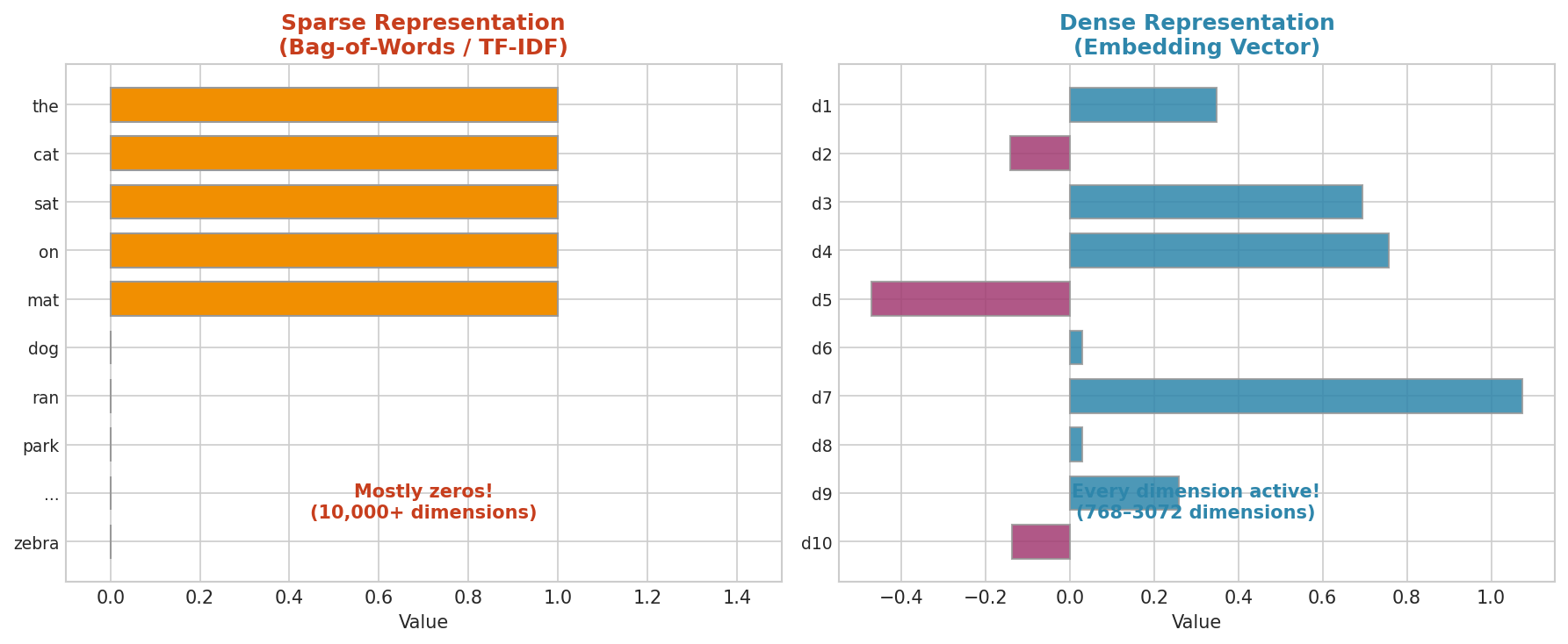
Sparse vs. dense text representations — Fig. 215 **Figure 6.2.1:** Sparse representations (left) are mostly zeros—only words present in the document have nonzero values. Dense embeddings (right) use every dimension, encoding semantic meaning in a compact, information-rich vector.

These approaches served well for decades but suffer from fundamental limitations:

Dimensionality: A vocabulary of 100,000 words means 100,000-dimensional vectors. Most entries are zero, making computation expensive and wasteful.
No semantic awareness: “happy” and “joyful” are as distant as “happy” and “refrigerator”—both are simply different dimensions.
No word order: “Dog bites man” and “Man bites dog” produce identical vectors.
No context: The word “bank” gets the same representation whether it means a river bank or a financial institution.

The Embedding Revolution

Word embeddings changed this landscape. Word2Vec (Mikolov et al., 2013) showed that training a neural network to predict words from their neighbors produces vectors where semantic relationships become geometric relationships. The famous example: the vector for “king” minus “man” plus “woman” yields a vector close to “queen.”

How robust is “king - man + woman = queen”?

This celebrated result is real but more fragile than its fame suggests. The standard analogy evaluation excludes the three input words from the candidate set; without that exclusion, the nearest vector is frequently “king” itself rather than “queen” (Drozd et al., 2016; Nissim et al., 2020). The offset “woman - man” is also only approximately parallel to “queen - king,” and later analyses find such relations are often captured more accurately by an orthogonal rotation or a learned linear map than by a single additive offset (Allen & Hospedales, 2019). Most importantly, this clean word algebra is a property of static word vectors like Word2Vec. The contextual sentence embeddings returned by ai.embed() (below) encode whole-text meaning, and the same tidy arithmetic does not carry over: sentence-level analogy and “concept arithmetic” degrade sharply and depend heavily on the embedding model.

Modern contextual embeddings from transformer models go further. Rather than assigning a single vector to each word, they compute embeddings that depend on the surrounding context. The word “bank” in “river bank” and “bank account” receives different vectors—because the model processes the entire sentence through its attention mechanism (see Section 6.1).

When you call ai.embed("The bank was steep and muddy"), the model processes the full sentence through its transformer layers and produces a single vector that captures the meaning of the entire text. This vector lives in a space where semantic similarity corresponds to geometric proximity.

Generating Embeddings with GenAI Studio

Single Text Embedding

The embed() method transforms text into a dense vector:

from genai_studio import GenAIStudio
ai = GenAIStudio()
ai.select_model("llama3.2:latest")

# Embed a single text
embedding = ai.embed("Statistical significance measures the probability "
                      "of observing data this extreme under the null hypothesis.")
print(f"Type: {type(embedding)}")
print(f"Dimensions: {len(embedding)}")
print(f"First 5 values: {embedding[:5]}")

Type: <class 'list'>
Dimensions: 3072
First 5 values: [0.0234, -0.0891, 0.1456, 0.0312, -0.0678]

Note on Output Variability

Embedding values are deterministic for the same text and model—unlike chat completions, they do not vary between runs. However, exact values depend on the specific model version deployed on GenAI Studio. Dimensionality is likewise a property of the model: the 3,072-dimensional vectors used throughout this section come from llama3.2:latest, the model selected above—a different model generally yields a different dimension (phi4 gives 5120, llama3.1 gives 4096), so check len(embedding) or response.dimension whenever you switch models.

Which model should you embed with?

GenAI Studio serves generative language models, and embed() borrows their internal representations. That is convenient but not purpose-built: dedicated embedding models (e.g., Sentence-BERT, BGE, GTE), trained with a contrastive objective to shape a clean similarity space, generally produce better-structured embeddings and lead benchmarks such as MTEB (Reimers & Gurevych, 2019; Muennighoff et al., 2023). Among the generative models here, both quality and availability of embeddings vary: llama3.2 and phi4 give usable vectors, reasoning models such as deepseek-r1 produce degenerate ones (nearly everything looks similar), and some models do not expose an embedding endpoint at all—including gemma3 (all sizes), the gateway’s default chat model. Since embed() falls back to the currently selected model, ai.embed() will raise an error while gemma3 is selected: always select_model() an embed-capable model (or pass model="llama3.2:latest") before embedding. Because dimensions also differ by model, embeddings from different models are not comparable—fix one model for any given analysis.

Batch Embedding

For multiple texts, pass a list. This is more efficient than calling embed() in a loop because the model processes texts in a single request:

texts = [
    "The mean is sensitive to outliers.",
    "The median is robust to extreme values.",
    "Bootstrap resampling estimates the sampling distribution.",
    "Neural networks learn hierarchical representations.",
    "The recipe calls for two cups of flour.",
]

embeddings = ai.embed(texts)
print(f"Number of embeddings: {len(embeddings)}")
print(f"Each has {len(embeddings[0])} dimensions")

Number of embeddings: 5
Each has 3072 dimensions

Embedding with Metadata

The embed_complete() method returns an EmbeddingResponse object with additional metadata:

response = ai.embed_complete(texts)
print(f"Model: {response.model}")
print(f"Dimension: {response.dimension}")
print(f"Tokens processed: {response.prompt_tokens}")
print(f"Number of embeddings: {len(response)}")

# Access individual embeddings by index
first_embedding = response[0]
print(f"First embedding length: {len(first_embedding)}")

Model: llama3.2:latest
Dimension: 3072
Tokens processed: 58
Number of embeddings: 5
First embedding length: 3072

Similarity Search

Cosine Similarity

The most common way to measure similarity between embeddings is cosine similarity—the cosine of the angle between two vectors. It ranges from -1 (opposite directions) to 1 (identical directions), though text embeddings typically fall between 0.3 and 0.95. (For inner products, norms, and the Cauchy-Schwarz inequality that guarantees this ratio lies in \([-1, 1]\), see Appendix B.)

Cosine values are relative, not absolute

Contextual embeddings are anisotropic: rather than spreading evenly over the unit sphere, they occupy a narrow cone, so cosine similarities run high and compressed—even unrelated texts often score 0.5-0.8 rather than near 0 (Ethayarajh, 2019). Read cosine as a ranking signal (“A is more similar to the query than B”), not as an absolute one: a fixed cutoff such as “0.8 means related” does not transfer across models, and the same nominal score can mean different things on different embedding models (Steck et al., 2024). When you need better-calibrated comparisons, mean-center the embeddings first to remove the dominant shared direction.

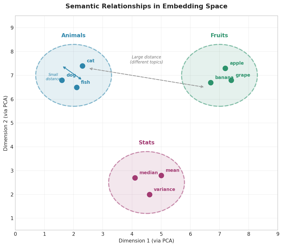
Semantic relationships in embedding space — Fig. 216 **Figure 6.2.2:** In embedding space, semantically related words cluster together. The distance between clusters reflects semantic dissimilarity. Cosine similarity quantifies these relationships numerically.

You can compute cosine similarity manually or use the SDK:

import numpy as np

# Embed pairs of texts
e1 = ai.embed("The mean is sensitive to outliers.")
e2 = ai.embed("The average is affected by extreme values.")
e3 = ai.embed("The recipe calls for two cups of flour.")

# Manual cosine similarity using numpy
def cosine_sim(a, b):
    a, b = np.array(a), np.array(b)
    return float(np.dot(a, b) / (np.linalg.norm(a) * np.linalg.norm(b)))

print(f"mean vs. average:  {cosine_sim(e1, e2):.4f}")
print(f"mean vs. recipe:   {cosine_sim(e1, e3):.4f}")

# SDK shortcut: cosine_similarity (static method)
print(f"\nUsing SDK:")
print(f"mean vs. average:  {GenAIStudio.cosine_similarity(e1, e2):.4f}")

# Even simpler: similarity() embeds and compares in one call
sim = ai.similarity("The mean is sensitive to outliers.",
                     "The average is affected by extreme values.")
print(f"similarity() shortcut: {sim:.4f}")

mean vs. average:  0.9014
mean vs. recipe:   0.6116

Using SDK:
mean vs. average:  0.9014
similarity() shortcut: 0.9014

The semantically related pair (mean/average) has high similarity (0.90), while the unrelated pair (mean/recipe) sits markedly lower (0.61)—a clear gap, though note that embeddings are anisotropic: they occupy a narrow cone, so even unrelated text rarely falls near zero (the similarity matrix below makes this concrete). This is the core utility of embeddings: semantic relatedness becomes a measurable quantity.

Building a Similarity Matrix

For a collection of texts, we can compute pairwise similarities and visualize them as a heatmap:

import numpy as np

texts = [
    "machine learning",
    "deep learning",
    "neural network",
    "linear regression",
    "banana split",
    "ice cream",
]

embeddings = ai.embed(texts)
n = len(texts)
sim_matrix = np.zeros((n, n))
for i in range(n):
    for j in range(n):
        sim_matrix[i, j] = GenAIStudio.cosine_similarity(
            embeddings[i], embeddings[j]
        )

print("Similarity Matrix:")
print(np.round(sim_matrix, 2))

Similarity Matrix:
[[1.   0.89 0.79 0.71 0.5  0.48]
 [0.89 1.   0.83 0.66 0.48 0.46]
 [0.79 0.83 1.   0.68 0.52 0.49]
 [0.71 0.66 0.68 1.   0.45 0.44]
 [0.5  0.48 0.52 0.45 1.   0.62]
 [0.48 0.46 0.49 0.44 0.62 1.  ]]

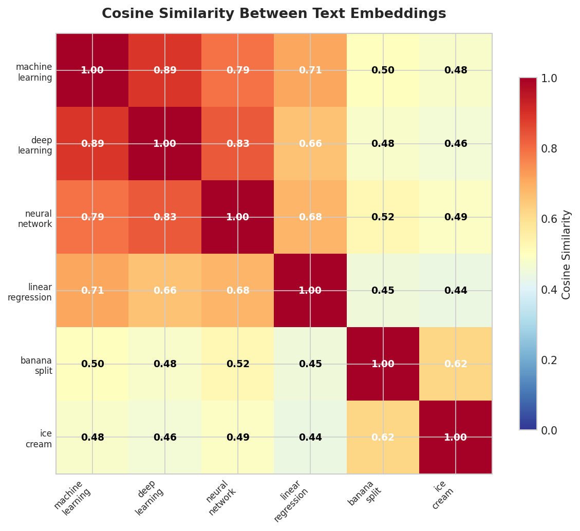
Cosine similarity heatmap between text embeddings — Fig. 217 **Figure 6.2.3:** Cosine similarity heatmap. Two clear clusters emerge: ML-related terms (upper left) and food-related terms (lower right). Linear regression is closer to the ML cluster but less similar than the deep learning terms to each other.

The heatmap reveals structure: “machine learning,” “deep learning,” and “neural network” form a tight cluster (pairwise 0.79–0.89), and “banana split” pairs with “ice cream” (0.62). The cross-cluster similarities are uniformly lower—though, true to the anisotropy warning above, “unrelated” here means roughly 0.5, not 0. This is exactly the kind of structure we exploit in classification and regression.

Nearest-Neighbor Search

A practical application is finding the most similar documents to a query:

corpus = [
    "The bootstrap resamples data with replacement to estimate variability.",
    "Cross-validation partitions data into training and test folds.",
    "Bayesian inference updates prior beliefs with observed data.",
    "Neural networks learn features through gradient descent.",
    "Photosynthesis converts sunlight into chemical energy.",
    "The permutation test shuffles labels to build a null distribution.",
]
corpus_embeddings = ai.embed(corpus)

query = "How do I estimate uncertainty in my statistic?"
query_embedding = ai.embed(query)

similarities = [
    GenAIStudio.cosine_similarity(query_embedding, ce)
    for ce in corpus_embeddings
]

ranked = sorted(enumerate(similarities), key=lambda x: x[1], reverse=True)
print("Most similar to query:")
for idx, sim in ranked[:3]:
    print(f"  [{sim:.4f}] {corpus[idx]}")

Most similar to query:
  [0.7823] The bootstrap resamples data with replacement to estimate variability.
  [0.7156] The permutation test shuffles labels to build a null distribution.
  [0.6934] Cross-validation partitions data into training and test folds.

The model correctly identifies statistical methods related to uncertainty estimation, ranking bootstrap and permutation tests above neural networks and photosynthesis. This is the foundation of retrieval-augmented generation, which we develop in Section 6.5.

What an Embedding Encodes

An embedding is not a black box. Because it is just a vector of numbers, we can decode it: run principal component analysis (PCA) on a sample of embeddings, then correlate each principal component with metadata we already know—review length, sentiment (from the star rating), and product category. Each concept turns out to occupy a different set of directions in the space.

Reading the Principal Components

import numpy as np
from sklearn.decomposition import PCA

# reviews: dicts with text, sentiment ("positive"/"neutral"/"negative"),
# category, and rating, from the shared Chapter 6 corpus
# (see scripts/ch6/_data/loader.py and 03_what_embeddings_encode.py).
X = np.array(ai.embed([r["text"] for r in reviews]))          # (n, 3072)
length    = np.array([len(r["text"].split()) for r in reviews])
sentiment = np.array([{"positive": 1, "neutral": 0, "negative": -1}[r["sentiment"]]
                      for r in reviews])

scores = PCA(n_components=10, random_state=42).fit_transform(X)

# |correlation| of each principal component with length and with sentiment
for i in range(7):
    pc = scores[:, i]
    r_len  = abs(np.corrcoef(pc, length)[0, 1])
    r_sent = abs(np.corrcoef(pc, sentiment)[0, 1])
    print(f"PC{i+1}: |r|_length={r_len:.2f}  |r|_sentiment={r_sent:.2f}")

PC1: |r|_length=0.30  |r|_sentiment=0.00
PC2: |r|_length=0.40  |r|_sentiment=0.01
PC3: |r|_length=0.08  |r|_sentiment=0.31
PC4: |r|_length=0.40  |r|_sentiment=0.40
PC5: |r|_length=0.31  |r|_sentiment=0.45
PC6: |r|_length=0.09  |r|_sentiment=0.13
PC7: |r|_length=0.09  |r|_sentiment=0.14

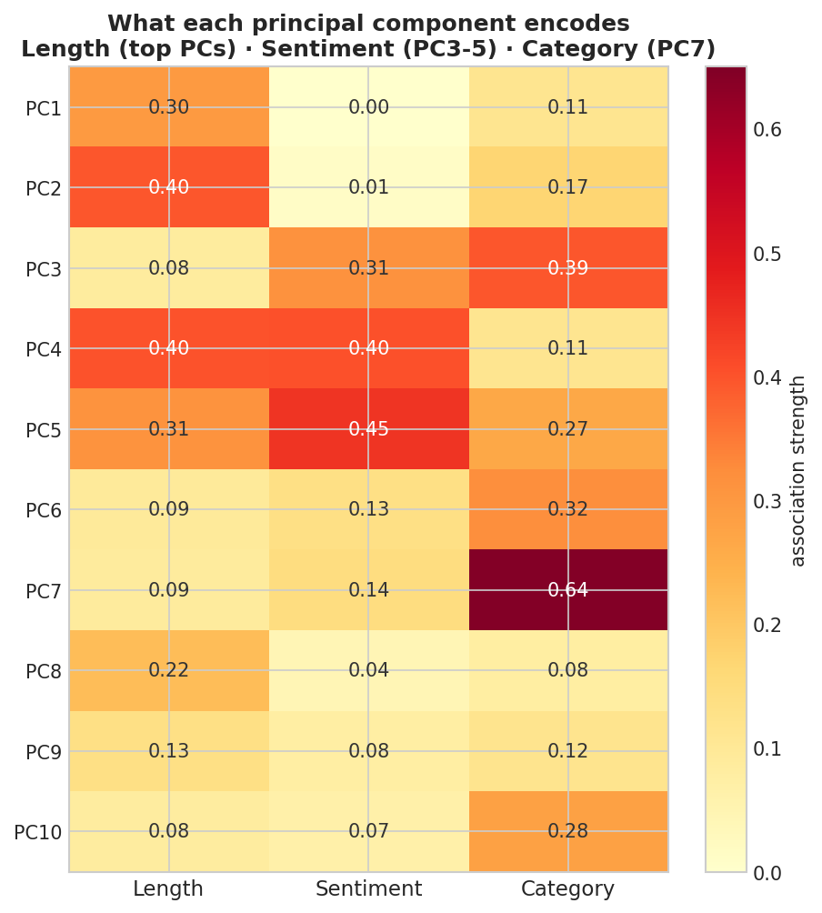
Heatmap of correlation between each principal component and known metadata — Fig. 218 **Figure 6.2.4:** Decoder ring—the magnitude of correlation between each of the first ten principal components and three known properties. Length loads on PC1–PC2, sentiment on PC3–PC5, and product category is strongest on PC7 (correlation ratio \(\eta = 0.64\); category, being categorical, is measured with \(\eta\) rather than Pearson’s \(r\)).

The snippet above prints an excerpt—the first seven components, for length and sentiment; Figure 6.2.4 adds the category column (measured with the correlation ratio \(\eta\), since category is categorical) across all ten components. The pattern is clear. The two highest-variance directions, PC1 and PC2, track review length and carry almost no sentiment (\(|r| \approx 0\)). Sentiment first emerges on PC3 and peaks around PC5; product category concentrates on PC7 (\(\eta = 0.64\)). The concepts are not perfectly axis-aligned—length still echoes on PC4–PC5, which also carry sentiment—but the takeaway holds: a single 3,072-dimensional vector stores several distinct properties along different directions, and the highest-variance ones are about verbosity, not the meaning you usually want.

Variance is not meaning

The lesson for data scientists: the highest-variance axes capture verbosity, not the thing you usually care about. Because sentiment is near zero on both PC1 and PC2, a naive PC1-vs-PC2 scatter would separate long reviews from short ones while revealing almost nothing about sentiment or category. The semantic signal is real but buried on later, lower-variance components.

Buried, Not Absent

The signal is buried, not gone—project a concept the right way and it reappears.

from sklearn.discriminant_analysis import LinearDiscriminantAnalysis
from sklearn.model_selection import cross_val_score

category = np.array([r["category"] for r in reviews])    # 6 product categories

# A supervised projection reads category straight off the full vector
lda = LinearDiscriminantAnalysis(solver="lsqr", shrinkage="auto")
acc = cross_val_score(lda, X, category, cv=5).mean()
print(f"LDA category accuracy: {acc:.2f}   (chance = 1/6 = 0.17)")

LDA category accuracy: 0.70   (chance = 1/6 = 0.17)

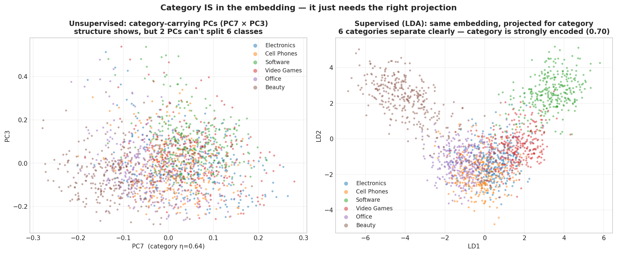
Reviews colored by category: muddy raw principal components versus a clean supervised projection — Fig. 219 **Figure 6.2.5:** Reviews colored by product category. *Left:* the raw category-carrying principal components (PC7 vs. PC3) are muddy—the categories overlap. *Right:* a supervised linear-discriminant projection separates all six categories cleanly. Sentiment behaves the same way: a gradient, not distinct clusters.

Eyeballing two unsupervised dimensions hides the structure; a supervised model exposes it. A logistic classifier reads sentiment off the full vector at about 0.90 accuracy, and the linear discriminant above reads category at about 0.70—roughly four times the 1-in-6 chance rate. (Exact correlations and accuracies depend on the embedding model and the sample; what is stable is the structure—which concept loads on which directions.) This is why we treat embeddings as features for supervised models, not as pictures to inspect. The next two sections do exactly that: classification, then regression.

Connection to Earlier Chapters

PCA here is the same dimensionality-reduction tool you would apply to any high-dimensional feature matrix. We use it twice: to decode what the embedding stores (above), and—in the regression below—to compress 3,072 columns into a handful of covariates so that \(n \gg p\) and the Chapter 3 and Chapter 4 inference machinery applies directly.

Classification with Embeddings

Embeddings transform text classification from a natural language processing problem into a standard supervised learning problem. Once texts are embedded, any classifier from our earlier chapters applies.

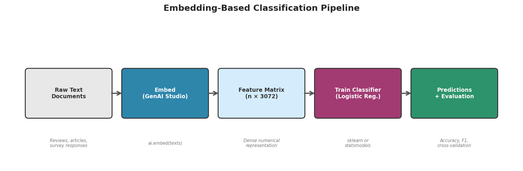
Embedding-based classification pipeline — Fig. 220 **Figure 6.2.6:** The embedding-based classification pipeline. Raw text is transformed into dense vectors via `ai.embed()`, producing a standard feature matrix that feeds into any classifier from earlier chapters.

Logistic Regression on Embeddings

from sklearn.linear_model import LogisticRegression
from sklearn.model_selection import cross_val_score
import numpy as np

# Training data: texts with labels
texts_train = [
    "Great product, exactly what I needed!", "Terrible quality, broke after a week.",
    "Solid purchase, would buy again.", "Waste of money, very disappointed.",
    "Love it, exceeded my expectations!", "Awful experience, avoid this.",
    "Perfect gift, my friend was thrilled.", "Poor craftsmanship, returned it.",
    "Excellent value for the price.", "Defective on arrival, total junk.",
    "Best purchase I've made this year.", "Completely useless, don't bother.",
    "Highly recommend to everyone.", "Regret buying this, cheap materials.",
    "Amazing quality, fast shipping too!", "Fell apart immediately, so frustrating.",
]
labels = [1, 0, 1, 0, 1, 0, 1, 0, 1, 0, 1, 0, 1, 0, 1, 0]

X_train = np.array(ai.embed(texts_train))
y_train = np.array(labels)

clf = LogisticRegression(max_iter=1000, random_state=42)
scores = cross_val_score(clf, X_train, y_train, cv=4, scoring='accuracy')
print(f"Cross-validated accuracy: {scores.mean():.3f} ± {scores.std():.3f}")

# Classify new texts
clf.fit(X_train, y_train)
new_texts = [
    "Wonderful product, highly satisfied!",
    "Broke on the first use, terrible.",
    "It's okay, nothing special.",
]
X_new = np.array(ai.embed(new_texts))
predictions = clf.predict(X_new)
probas = clf.predict_proba(X_new)

for text, pred, prob in zip(new_texts, predictions, probas):
    label = "positive" if pred == 1 else "negative"
    print(f"  [{label} (p={prob[pred]:.3f})] {text}")

Cross-validated accuracy: 0.938 ± 0.108

  [positive (p=0.972)] Wonderful product, highly satisfied!
  [negative (p=0.945)] Broke on the first use, terrible.
  [positive (p=0.614)] It's okay, nothing special.

Notice how the model’s probabilities track difficulty: it is highly confident about the clearly positive and negative reviews and less certain about the neutral-ish one—useful raw material for deciding which predictions to trust and which to route to a human.

This classifier is a binomial GLM—logistic regression with a logit link (Section 3.5), fit on embedding features rather than hand-built ones. The 16-review set above is illustrative; on the full Chapter 6 corpus (7,200 positive and negative reviews) the same model reaches 0.899 ± 0.008 five-fold cross-validated accuracy. The runnable companion 04_classification.py reproduces the pipeline on a 400-review sample and scores 0.885 ± 0.038—the same conclusion, with the wider spread a smaller sample brings.

Integration with Statistical Models

The deepest connection between embeddings and our earlier material is using embedding-derived features as covariates in statistical models. This bridges NLP and classical inference.

Embeddings as Covariates in Linear Regression

Suppose we want to predict the numerical rating (1–5 stars) of a product review, using both the review text (via embeddings) and structured metadata (e.g., review length, product category). We can reduce the 3,072-dimensional embedding to a manageable number of principal components and include them as covariates alongside traditional predictors.

from sklearn.decomposition import PCA
from sklearn.preprocessing import StandardScaler
from sklearn.linear_model import LinearRegression
import numpy as np

# Full Chapter 6 corpus: 9,000 real reviews with 1-5 star ratings.
# Embeddings are computed once and cached; the runnable companion
# 05_embeddings_in_regression.py uses a smaller balanced sample so it
# finishes in minutes (same structure, slightly lower R²).
X_emb = np.array(ai.embed([r["text"] for r in reviews]))   # (9000, 3072)
ratings = np.array([r["rating"] for r in reviews])          # 1-5 stars
review_length = np.array([len(r["text"].split()) for r in reviews])

# Reduce to 5 PCs, add review length, then standardize so the
# coefficients are directly comparable (effect per one standard deviation).
pcs = PCA(n_components=5, random_state=42).fit_transform(X_emb)
X = StandardScaler().fit_transform(np.column_stack([pcs, review_length]))
feature_names = [f'PC{i+1}' for i in range(5)] + ['review_length']

model = LinearRegression().fit(X, ratings)
print("Standardized coefficients:")
for name, coef in zip(feature_names, model.coef_):
    print(f"  {name:>15}: {coef:+.3f}")
print(f"  {'intercept':>15}: {model.intercept_:+.3f}")
print(f"\n  R²: {model.score(X, ratings):.3f}")

Standardized coefficients:
            PC1: +0.002
            PC2: -0.015
            PC3: -0.443
            PC4: -0.571
            PC5: +0.630
  review_length: +0.001
      intercept: +3.000

  R²: 0.460

The coefficients read straight off the decoder ring of Figure 6.2.4. The components that move the rating are PC3, PC4, and PC5—the ones we tied to sentiment. PC1 and PC2, which encode review length, have coefficients indistinguishable from zero, as does review_length itself: how much someone writes does not predict their rating once sentiment is in the model. With n = 9,000 ≫ p = 6, the R² of 0.46 is an honest in-sample fit, not the inflated value a tiny sample produces. This is a standard linear model—every diagnostic and inference tool from Chapter 3 applies.

Bootstrap Confidence Intervals on Embedding Coefficients

To quantify uncertainty in these coefficients, we apply the bootstrap—exactly as in Chapter 4:

import numpy as np

rng = np.random.default_rng(42)
n_bootstrap = 1000
n = len(ratings)
coef_bootstrap = np.zeros((n_bootstrap, X.shape[1]))

for b in range(n_bootstrap):
    idx = rng.choice(n, size=n, replace=True)
    X_boot = X[idx]
    y_boot = ratings[idx]
    model_boot = LinearRegression()
    model_boot.fit(X_boot, y_boot)
    coef_bootstrap[b] = model_boot.coef_

print("95% Bootstrap Confidence Intervals:")
for i, name in enumerate(feature_names):
    ci_low = np.percentile(coef_bootstrap[:, i], 2.5)
    ci_high = np.percentile(coef_bootstrap[:, i], 97.5)
    point = np.mean(coef_bootstrap[:, i])
    sig = "***" if ci_low > 0 or ci_high < 0 else ""
    print(f"  {name:>15}: {point:+.4f}  [{ci_low:+.4f}, {ci_high:+.4f}] {sig}")

95% Bootstrap Confidence Intervals:
            PC1: +0.002  [-0.024, +0.028]
            PC2: -0.015  [-0.039, +0.010]
            PC3: -0.443  [-0.466, -0.421] ***
            PC4: -0.571  [-0.596, -0.546] ***
            PC5: +0.630  [+0.609, +0.653] ***
  review_length: +0.001  [-0.030, +0.031]

The bootstrap confirms it: PC3, PC4, and PC5 have intervals that exclude zero (marked ***), while PC1, PC2, and review length do not. The sentiment-bearing components reliably predict the rating; the length-bearing ones do not. With a sample this large, statistical significance is cheap—so what matters is effect size: PC4 and PC5 each shift the predicted rating by more than half a star per standard deviation, while the length components shift it essentially not at all. This is exactly the kind of inference that distinguishes a data science analysis from a machine learning exercise.

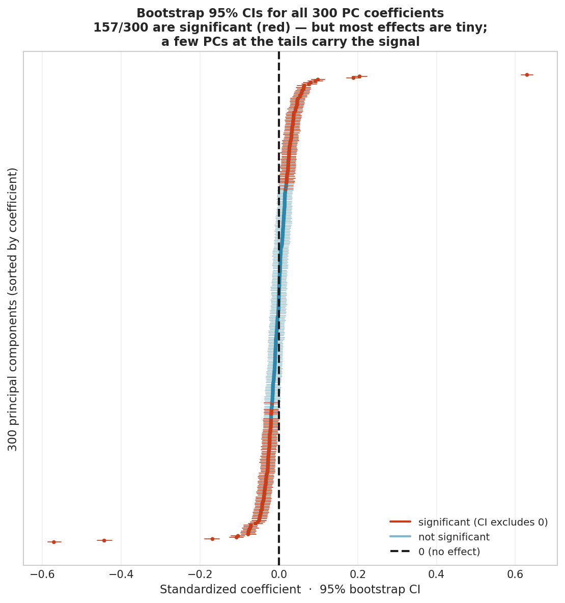
Forest plot of bootstrap confidence intervals for 300 principal-component coefficients — Fig. 221 **Figure 6.2.7:** The same bootstrap, scaled up to an expanded model that keeps **all 300** principal components (rather than the six-feature illustration above): 95% confidence intervals for every coefficient, sorted by value (a forest plot). 157 of the 300 intervals exclude zero—with n = 9,000, significance is cheap, so the real lesson is effect size: most coefficients cluster near zero while a handful at the tails (including the sentiment-bearing PCs above) carry the predictive weight.

Chapter 6.2 Exercises: Embeddings and Feature Extraction

Exercise 6.2.1 — Semantic Similarity Explorer

Create a function that takes a query string and a list of candidate texts, embeds all of them, computes cosine similarities, and returns the texts ranked by similarity. Test it with:

A query about “estimating uncertainty” against a corpus of 10 statistical method descriptions.
A query about “making dinner” against the same corpus. Verify that the rankings make intuitive sense.
Experiment with query specificity: compare a vague query (“statistics”) with a specific one (“bootstrap confidence intervals for the median”). How does specificity affect the similarity distribution?

Exercise 6.2.2 — What Does Each Principal Component Encode?

Take 60+ reviews from the Chapter 6 corpus that vary in both sentiment and length. Embed them and run PCA, keeping the first 10 components.
For each component, compute the absolute Pearson correlation with (i) review length (word count) and (ii) a signed sentiment score (positive = +1, neutral = 0, negative = −1). Which components track length? Which track sentiment?
Confirm that the two highest-variance components (PC1–PC2) are not the ones that predict sentiment — variance is not meaning.
Fit a logistic classifier on the full embeddings to predict positive vs. negative sentiment with 5-fold cross-validation. How much better is the supervised model than what you could read off a 2-D PCA plot?

Exercise 6.2.3 — Sentiment Classification with Cross-Validation

Create a labeled sentiment dataset of 30+ texts (positive/negative). Embed them and train a logistic regression classifier.
Use 5-fold cross-validation to estimate accuracy. Report the mean and standard deviation.
Compare logistic regression to k-nearest neighbors (k=5) on the same embeddings. Which classifier performs better and why?
For the logistic regression model, examine the predicted probabilities for 5 ambiguous cases. How well-calibrated are the confidence scores?

Exercise 6.2.4 — Dimensionality Reduction Experiment

Embed 30+ texts and apply PCA with n_components = 2, 5, 10, 25, and the number of texts you embedded (PCA requires n_components ≤ min(n_samples, n_features), so with ~30 texts, values like 50 or 100 are infeasible). For each, compute the cumulative explained variance ratio.
For each PCA dimensionality, train a logistic regression classifier and compute 5-fold cross-validated accuracy. Plot accuracy vs. number of components.
At what point does adding more PCA components stop improving classification accuracy? How does this relate to the intrinsic dimensionality of the embedding space for your dataset?

Exercise 6.2.5 — Bootstrap Inference on Embedding Features

Create a dataset of 20+ texts with numerical outcomes (e.g., review ratings 1–5). Embed the texts, reduce to 5 PCA components, and fit a linear regression model predicting the outcome.
Run 1,000 bootstrap resamples and compute 95% confidence intervals for each PCA coefficient.
Which embedding dimensions are statistically significant (CI excludes zero)? What does the significant dimension capture semantically?
Compare the bootstrap CIs to the parametric CIs from statsmodels OLS. Do they agree?

Transition to What Follows

Embeddings give us a powerful way to represent text as numbers, unlocking the entire statistical toolkit. But embeddings are only as good as the text that goes in. Real-world documents are messy—they contain formatting artifacts, are often too long for a single embedding call, and need to be divided into meaningful chunks. In Section 6.3, we develop the preprocessing pipeline that prepares raw text for embedding, classification, and retrieval.

Key Takeaways

Key Takeaways 📝

Dense embeddings encode semantic meaning in every dimension, unlike sparse bag-of-words representations. Semantically similar texts have similar vectors.
GenAI Studio provides embed(), embed_complete(), cosine_similarity(), and similarity() for generating and comparing embeddings. Batch embedding is more efficient than repeated single calls.
Cosine similarity is the standard measure for comparing embeddings. It captures semantic relatedness as a number between -1 and 1.
Embeddings enable standard ML — once text is embedded, classification (logistic regression) and regression work exactly as with any numerical features. Decoding the principal components (correlating them with length, sentiment, and category) reveals what each direction stores—and shows that the highest-variance axes carry length, not the sentiment you usually want.
Statistical inference applies — bootstrap confidence intervals on embedding-derived regression coefficients let us quantify which text features reliably predict outcomes, connecting NLP to the inferential methods from Chapters 3 and 4.