Appendix B: Linear Algebra for Data Science
From Notation to Intuition
Linear algebra is the language of modern statistics and data science. Every dataset is a matrix, every model parameter is a vector, and every inference procedure — from ordinary least squares to MCMC — is a sequence of matrix operations. Yet students often arrive with linear algebra as a collection of mechanical rules (multiply rows by columns, compute determinants by cofactor expansion) without the geometric intuition that makes statistical applications natural.
This appendix bridges that gap. We develop the linear algebra prerequisites for this course with emphasis on why each concept matters for statistical computation, not just what the formulas are. The goal is to build the geometric reasoning that lets you read a matrix expression like \(\mathbf{H} = \mathbf{X}(\mathbf{X}^\top\mathbf{X})^{-1}\mathbf{X}^\top\) and immediately see a projection — the operation that finds the closest point in a subspace to a given vector, which is precisely what least squares does.
Road Map 🧭
Foundations: Vectors, matrices, and the operations that connect them — with emphasis on the properties that matter for statistics
Structure: Special matrix types (symmetric, positive definite, idempotent, stochastic) that arise naturally in statistical models
Blocks: Partitioned matrices, the Schur complement, and the Sherman-Morrison-Woodbury formula — tools for working with structured problems
Geometry: Column spaces, projections, and the hat matrix — the geometric engine behind least squares
Decompositions: Eigen, Cholesky, QR, and SVD — each revealing different structure in data and models
Covariance: Quadratic forms and covariance matrices — how variance propagates through linear transformations via \(\text{Var}(\mathbf{A}\mathbf{X}) = \mathbf{A}\text{Var}(\mathbf{X})\mathbf{A}^\top\)
Calculus: Gradients of scalar functions of vectors and matrices — the foundation for optimization-based inference
Computation: Numerical considerations — condition numbers, when to avoid forming \(\mathbf{X}^\top\mathbf{X}\), and why decompositions beat direct inversion
Prerequisites Check ✓
Before proceeding, ensure you’re comfortable with:
Systems of linear equations and their solution
The concept of a function and composition of functions
Basic calculus (derivatives, partial derivatives)
Python basics and NumPy arrays
Connection to Course Material 🗺️
This appendix supports specific course content:
Chapter 2 (Monte Carlo): Cholesky decomposition for generating correlated random vectors (Section 2.4 Transformation Methods (Optional))
Chapter 3 (Parametric Inference): Hat matrix, projections, QR decomposition in linear models (Section 3.4 Linear Models); Fisher information matrices (Section 3.2 Maximum Likelihood Estimation); IRLS weight matrices (Section 3.5 Generalized Linear Models)
Chapter 4 (Resampling): Sherman-Morrison-Woodbury for LOOCV shortcuts (Section 4.8: Cross-Validation Methods (Optional)); influence diagnostics via the hat matrix (Section 4.5: Jackknife Methods (Optional))
Chapter 5 (Bayesian): Transition matrices for Markov chains (Section 5.4 Markov Chains: The Mathematical Foundation of MCMC); mass matrix in Hamiltonian Monte Carlo (Section 5.5 MCMC Algorithms: Metropolis-Hastings and Gibbs Sampling)
Vectors and Inner Products
A vector \(\mathbf{x} \in \mathbb{R}^n\) is an ordered list of \(n\) real numbers. Throughout this course, vectors are column vectors by default:
The transpose \(\mathbf{x}^\top = (x_1, x_2, \ldots, x_n)\) gives a row vector.
Inner Product and Norm
Definition
The inner product (dot product) of two vectors \(\mathbf{x}, \mathbf{y} \in \mathbb{R}^n\) is:
The Euclidean norm (length) of a vector is:
The inner product measures how well two vectors align. When \(\mathbf{x}^\top \mathbf{y} = 0\), the vectors are orthogonal — they point in perpendicular directions. This geometric intuition is central to least squares: the residual vector is orthogonal to the space of fitted values.
Key Properties
Symmetry: \(\mathbf{x}^\top \mathbf{y} = \mathbf{y}^\top \mathbf{x}\)
Linearity: \(\mathbf{x}^\top(a\mathbf{y} + b\mathbf{z}) = a\,\mathbf{x}^\top \mathbf{y} + b\,\mathbf{x}^\top \mathbf{z}\)
Cauchy-Schwarz inequality: \(|\mathbf{x}^\top \mathbf{y}| \leq \|\mathbf{x}\| \cdot \|\mathbf{y}\|\), with equality if and only if \(\mathbf{x}\) and \(\mathbf{y}\) are linearly dependent
Triangle inequality: \(\|\mathbf{x} + \mathbf{y}\| \leq \|\mathbf{x}\| + \|\mathbf{y}\|\)
The Cauchy-Schwarz inequality appears in the derivation of the Cramér-Rao lower bound (see Section 3.2 Maximum Likelihood Estimation), where it establishes the minimum variance achievable by any unbiased estimator.
import numpy as np

x = np.array([3, 1, 4])
y = np.array([2, 7, 1])

# Inner product
dot = x @ y          # 17
dot_alt = np.dot(x, y)  # equivalent

# Norm
norm_x = np.linalg.norm(x)  # sqrt(26) ≈ 5.099

# Verify Cauchy-Schwarz
assert abs(x @ y) <= np.linalg.norm(x) * np.linalg.norm(y)
Orthogonality
Two vectors are orthogonal if \(\mathbf{x}^\top \mathbf{y} = 0\). A set of vectors \(\{\mathbf{q}_1, \ldots, \mathbf{q}_k\}\) is orthonormal if:
Equivalently, stacking these vectors as columns of a matrix \(\mathbf{Q}\), orthonormality means \(\mathbf{Q}^\top \mathbf{Q} = \mathbf{I}\). If \(\mathbf{Q}\) is square, this also gives \(\mathbf{Q}\mathbf{Q}^\top = \mathbf{I}\), so \(\mathbf{Q}^{-1} = \mathbf{Q}^\top\) — the inverse is just the transpose. Such a matrix is called orthogonal.
Orthogonal matrices preserve lengths and angles: \(\|\mathbf{Q}\mathbf{x}\| = \|\mathbf{x}\|\). This makes them numerically ideal — they never amplify errors, which is why QR decomposition is preferred over forming \(\mathbf{X}^\top\mathbf{X}\) directly.
Matrix Operations and Properties
A matrix \(\mathbf{A} \in \mathbb{R}^{m \times n}\) has \(m\) rows and \(n\) columns. We write \(A_{ij}\) or \(a_{ij}\) for the entry in row \(i\), column \(j\).
Multiplication, Transpose, and Inverse
Matrix multiplication. If \(\mathbf{A}\) is \(m \times n\) and \(\mathbf{B}\) is \(n \times p\), the product \(\mathbf{C} = \mathbf{AB}\) is \(m \times p\) with entries:
Key properties:
Not commutative: \(\mathbf{AB} \neq \mathbf{BA}\) in general
Associative: \((\mathbf{AB})\mathbf{C} = \mathbf{A}(\mathbf{BC})\)
Distributive: \(\mathbf{A}(\mathbf{B} + \mathbf{C}) = \mathbf{AB} + \mathbf{AC}\)
Transpose of product: \((\mathbf{AB})^\top = \mathbf{B}^\top \mathbf{A}^\top\) (order reverses)
Transpose. \((\mathbf{A}^\top)_{ij} = A_{ji}\) — rows become columns. A matrix is symmetric if \(\mathbf{A} = \mathbf{A}^\top\). Covariance matrices and Fisher information matrices are always symmetric.
Inverse. A square matrix \(\mathbf{A}\) is invertible (nonsingular) if there exists \(\mathbf{A}^{-1}\) such that \(\mathbf{A}\mathbf{A}^{-1} = \mathbf{A}^{-1}\mathbf{A} = \mathbf{I}\). Key properties:
\((\mathbf{AB})^{-1} = \mathbf{B}^{-1}\mathbf{A}^{-1}\) (order reverses)
\((\mathbf{A}^\top)^{-1} = (\mathbf{A}^{-1})^\top\)
\((\mathbf{A}^{-1})^{-1} = \mathbf{A}\)
Common Pitfall ⚠️
In practice, you almost never compute \(\mathbf{A}^{-1}\) explicitly. To solve \(\mathbf{A}\mathbf{x} = \mathbf{b}\), use np.linalg.solve(A, b) rather than np.linalg.inv(A) @ b. The solve approach is faster and more numerically stable because it uses LU factorization internally without forming the full inverse.
Trace
Definition
The trace of a square matrix \(\mathbf{A} \in \mathbb{R}^{n \times n}\) is the sum of its diagonal entries:
The trace has remarkably useful algebraic properties:
Linearity: \(\text{tr}(\mathbf{A} + \mathbf{B}) = \text{tr}(\mathbf{A}) + \text{tr}(\mathbf{B})\) and \(\text{tr}(c\mathbf{A}) = c \cdot \text{tr}(\mathbf{A})\)
Cyclic property: \(\text{tr}(\mathbf{ABC}) = \text{tr}(\mathbf{CAB}) = \text{tr}(\mathbf{BCA})\)
Transpose invariance: \(\text{tr}(\mathbf{A}^\top) = \text{tr}(\mathbf{A})\)
Inner product connection: \(\mathbf{x}^\top \mathbf{A} \mathbf{x} = \text{tr}(\mathbf{A}\mathbf{x}\mathbf{x}^\top)\)
The cyclic property is especially powerful. Note that while \(\text{tr}(\mathbf{ABC}) = \text{tr}(\mathbf{CAB})\), the trace is not invariant under arbitrary permutations: \(\text{tr}(\mathbf{ABC}) \neq \text{tr}(\mathbf{BAC})\) in general.
In linear models, the trace gives the effective degrees of freedom: \(\text{tr}(\mathbf{H}) = p\) for the hat matrix \(\mathbf{H}\), generalizing to \(\text{tr}(\mathbf{S}_\lambda)\) for smoothers and regularized estimators (see Section 4.8: Cross-Validation Methods (Optional)).
Determinant
The determinant \(\det(\mathbf{A})\) is a scalar that encodes the volume-scaling factor of the linear transformation represented by \(\mathbf{A}\). Key properties:
\(\det(\mathbf{A}) \neq 0\) if and only if \(\mathbf{A}\) is invertible
\(\det(\mathbf{AB}) = \det(\mathbf{A})\det(\mathbf{B})\)
\(\det(\mathbf{A}^\top) = \det(\mathbf{A})\)
\(\det(c\mathbf{A}) = c^n \det(\mathbf{A})\) for \(\mathbf{A} \in \mathbb{R}^{n \times n}\)
\(\det(\mathbf{A}^{-1}) = 1/\det(\mathbf{A})\)
For diagonal or triangular matrices, the determinant is simply the product of diagonal entries: \(\det(\mathbf{A}) = \prod_i A_{ii}\).
The determinant appears prominently in probability through the multivariate normal density:
where \(|\boldsymbol{\Sigma}| = \det(\boldsymbol{\Sigma})\). It also appears in the Jacobian formula for change of variables (see Jacobian and Change of Variables) and in log-likelihoods for multivariate models.
Rank
The rank of a matrix \(\mathbf{A} \in \mathbb{R}^{m \times n}\) is the dimension of its column space — equivalently, the maximum number of linearly independent columns (or rows). A matrix has full column rank if \(\text{rank}(\mathbf{A}) = n\) (all columns are linearly independent), and full row rank if \(\text{rank}(\mathbf{A}) = m\).
For the design matrix \(\mathbf{X} \in \mathbb{R}^{n \times p}\) in linear regression, the full rank assumption \(\text{rank}(\mathbf{X}) = p\) is equivalent to requiring that \(\mathbf{X}^\top\mathbf{X}\) is invertible. When this fails — due to perfect collinearity among predictors — the OLS estimator \((\mathbf{X}^\top\mathbf{X})^{-1}\mathbf{X}^\top\mathbf{y}\) does not exist, and regularization (ridge, LASSO) or variable selection is needed.
import numpy as np

A = np.array([[1, 2, 3],
               [4, 5, 6],
               [7, 8, 9]])

print(f"Rank: {np.linalg.matrix_rank(A)}")        # 2 (row 3 = 2*row2 - row1)
print(f"Determinant: {np.linalg.det(A):.6f}")      # ≈ 0 (singular)
print(f"Trace: {np.trace(A)}")                      # 15
Special Matrix Structures
Certain matrix structures arise repeatedly in statistics. Recognizing them unlocks computational shortcuts and theoretical insights. Several of the properties below are stated in terms of eigenvalues — the scalars \(\lambda\) satisfying \(\mathbf{A}\mathbf{v} = \lambda \mathbf{v}\) for some nonzero eigenvector \(\mathbf{v}\), so that \(\mathbf{A}\) acts on \(\mathbf{v}\) by pure scaling. Eigenvalues are developed fully in the Spectral Theorem (see Matrix Decompositions below); for now, the defining equation is all we need.
Symmetric Matrices
A matrix \(\mathbf{A}\) is symmetric if \(\mathbf{A} = \mathbf{A}^\top\). Every covariance matrix, every Fisher information matrix, and every Hessian of a smooth function is symmetric. Symmetric matrices have three important properties:
All eigenvalues are real (not complex)
Eigenvectors corresponding to distinct eigenvalues are orthogonal
Every symmetric matrix admits a spectral decomposition \(\mathbf{A} = \mathbf{Q}\boldsymbol{\Lambda}\mathbf{Q}^\top\) with orthogonal \(\mathbf{Q}\)
These properties are the foundation of principal component analysis (PCA) and the spectral analysis of Markov chains.
Diagonal and Identity Matrices
A diagonal matrix \(\mathbf{D} = \text{diag}(d_1, \ldots, d_n)\) has nonzero entries only on the main diagonal. Diagonal matrices are trivial to invert (\(\mathbf{D}^{-1} = \text{diag}(1/d_1, \ldots, 1/d_n)\)) and their determinant is \(\prod_i d_i\).
The identity matrix \(\mathbf{I}_n\) is the diagonal matrix with all ones — the multiplicative identity: \(\mathbf{AI} = \mathbf{IA} = \mathbf{A}\).
In GLM fitting, the weight matrix \(\mathbf{W} = \text{diag}(w_1, \ldots, w_n)\) is diagonal, making the weighted least squares step \((\mathbf{X}^\top\mathbf{W}\mathbf{X})^{-1}\mathbf{X}^\top\mathbf{W}\mathbf{z}\) efficient to compute (see Section 3.5 Generalized Linear Models).
Idempotent Matrices
Definition
A matrix \(\mathbf{P}\) is idempotent if \(\mathbf{P}^2 = \mathbf{P}\).
Idempotency means “applying the operation twice is the same as applying it once” — the defining property of a projection. If you project a vector onto a subspace, projecting the result again changes nothing.
The hat matrix \(\mathbf{H} = \mathbf{X}(\mathbf{X}^\top\mathbf{X})^{-1}\mathbf{X}^\top\) is idempotent, and so is the residual-maker \(\mathbf{M} = \mathbf{I} - \mathbf{H}\).
Key properties of idempotent matrices:
Eigenvalues are either 0 or 1
\(\text{rank}(\mathbf{P}) = \text{tr}(\mathbf{P})\) (the trace counts the number of eigenvalue-1 directions)
If \(\mathbf{P}\) is also symmetric, it is an orthogonal projection matrix
Derivation: Eigenvalues of Idempotent Matrices
If \(\mathbf{P}\mathbf{v} = \lambda \mathbf{v}\) for eigenvector \(\mathbf{v} \neq \mathbf{0}\), then:
But \(\mathbf{P}^2 = \mathbf{P}\), so \(\mathbf{P}^2 \mathbf{v} = \mathbf{P}\mathbf{v} = \lambda \mathbf{v}\). Therefore \(\lambda^2 = \lambda\), which gives \(\lambda = 0\) or \(\lambda = 1\).
Positive Definite and Positive Semi-Definite Matrices
Definition
A symmetric matrix \(\mathbf{A} \in \mathbb{R}^{n \times n}\) is:
Positive definite (PD) if \(\mathbf{x}^\top \mathbf{A} \mathbf{x} > 0\) for all \(\mathbf{x} \neq \mathbf{0}\)
Positive semi-definite (PSD) if \(\mathbf{x}^\top \mathbf{A} \mathbf{x} \geq 0\) for all \(\mathbf{x}\)
Equivalently:
PD \(\iff\) all eigenvalues are strictly positive
PSD \(\iff\) all eigenvalues are non-negative
Positive definiteness is the matrix analogue of a positive number — it guarantees that a quadratic form \(\mathbf{x}^\top\mathbf{A}\mathbf{x}\) has a unique minimum at \(\mathbf{x} = \mathbf{0}\), which is essential for:
Covariance matrices: Every covariance matrix is PSD; it is PD if no variable is a deterministic linear combination of others
Fisher information matrices: PD under regularity conditions, ensuring the MLE is unique and the Cramér-Rao bound is finite
Hessians at optima: The Hessian of a log-likelihood being negative definite at \(\hat{\boldsymbol{\theta}}\) confirms a local maximum
Cholesky decomposition: A unique Cholesky factor with strictly positive diagonal exists if and only if the matrix is PD
import numpy as np

# A positive definite matrix
A = np.array([[4, 2],
               [2, 3]])

eigenvalues = np.linalg.eigvalsh(A)
print(f"Eigenvalues: {eigenvalues}")  # [1.438, 5.562] — both positive → PD

# Verify: x'Ax > 0 for random x
rng = np.random.default_rng(42)
for _ in range(1000):
    x = rng.standard_normal(2)
    assert x @ A @ x > 0
Stochastic Matrices
Definition
A square matrix \(\mathbf{P}\) is (row-)stochastic if:
All entries are non-negative: \(P_{ij} \geq 0\)
Each row sums to 1: \(\sum_j P_{ij} = 1\)
Stochastic matrices are transition matrices for Markov chains: \(P_{ij}\) is the probability of moving from state \(i\) to state \(j\). In Chapter 5, the \(k\)-step transition probabilities are given by \(\mathbf{P}^k\), and the stationary distribution \(\boldsymbol{\pi}\) satisfies \(\boldsymbol{\pi}^\top \mathbf{P} = \boldsymbol{\pi}^\top\) — it is a left eigenvector of \(\mathbf{P}\) with eigenvalue 1 (see Section 5.4 Markov Chains: The Mathematical Foundation of MCMC).
The Perron-Frobenius theorem guarantees that for an irreducible, aperiodic stochastic matrix, eigenvalue 1 has multiplicity one and all other eigenvalues satisfy \(|\lambda| < 1\). This ensures the Markov chain converges to a unique stationary distribution regardless of starting state — the theoretical foundation for MCMC.
Block Matrices
Many matrices in statistics have natural block structure. The design matrix might partition into \(\mathbf{X} = [\mathbf{X}_1 \mid \mathbf{X}_2]\) separating groups of predictors. A covariance matrix for two groups of variables decomposes into within-group and between-group blocks. Working with blocks rather than individual entries simplifies both algebra and computation.
Block Partitioning
A matrix can be partitioned into blocks (sub-matrices):
where \(\mathbf{A}_{11}\) is \(p \times p\), \(\mathbf{A}_{12}\) is \(p \times q\), \(\mathbf{A}_{21}\) is \(q \times p\), and \(\mathbf{A}_{22}\) is \(q \times q\).
Block Multiplication
Block matrices multiply according to the same row-times-column rule, but with sub-matrix products replacing scalar products:
This is valid whenever the inner dimensions of each sub-matrix product are compatible.
Block Transpose and Block Diagonal
The transpose of a block matrix transposes the arrangement and each block:
A block diagonal matrix has non-zero blocks only on the diagonal:
Block diagonal matrices are especially convenient: their inverse is \(\text{diag}(\mathbf{A}_1^{-1}, \ldots, \mathbf{A}_k^{-1})\), their determinant is \(\prod_i \det(\mathbf{A}_i)\), and their eigenvalues are the union of each block’s eigenvalues. They arise in hierarchical models where groups are conditionally independent.
The Schur Complement
Definition
Given a block matrix with \(\mathbf{A}_{11}\) invertible:
the Schur complement of \(\mathbf{A}_{11}\) in \(\mathbf{A}\) is:
The Schur complement is the key to block matrix inversion and appears throughout statistics:
Block inverse. If both \(\mathbf{A}_{11}\) and \(\mathbf{S}\) are invertible:
Block determinant:
Statistical Application: Conditional Distributions
For a multivariate normal \((\mathbf{X}_1, \mathbf{X}_2)^\top \sim \mathcal{N}(\boldsymbol{\mu}, \boldsymbol{\Sigma})\) with:
the conditional distribution \(\mathbf{X}_1 \mid \mathbf{X}_2 = \mathbf{x}_2\) is normal with:
The conditional covariance is exactly the Schur complement of \(\boldsymbol{\Sigma}_{22}\) in \(\boldsymbol{\Sigma}\). This formula drives Gibbs sampling for multivariate normals in Chapter 5.
Sherman-Morrison-Woodbury Formula
Theorem: Sherman-Morrison-Woodbury
If \(\mathbf{A} \in \mathbb{R}^{n \times n}\) and \(\mathbf{C} \in \mathbb{R}^{k \times k}\) are invertible, \(\mathbf{U} \in \mathbb{R}^{n \times k}\) and \(\mathbf{V} \in \mathbb{R}^{k \times n}\), and \(\mathbf{C}^{-1} + \mathbf{V}\mathbf{A}^{-1}\mathbf{U}\) is also invertible:
The special case with \(k = 1\) (rank-1 update) is the Sherman-Morrison formula: for vectors \(\mathbf{u}, \mathbf{v}\) with \(1 + \mathbf{v}^\top\mathbf{A}^{-1}\mathbf{u} \neq 0\):
This converts inverting an \(n \times n\) matrix into inverting a \(k \times k\) matrix (plus some matrix-vector products). When \(k \ll n\), this is a dramatic speedup.
The formula is central to the LOOCV shortcut in Section 4.8: Cross-Validation Methods (Optional): deleting observation \(i\) from the regression amounts to a rank-1 update of \(\mathbf{X}^\top\mathbf{X}\), allowing all \(n\) leave-one-out fits to be computed from a single full-data fit. It also appears in Bayesian posterior updating when a new observation arrives.
Derivation: Sherman-Morrison-Woodbury from Block Inversion
The formula follows from applying the block inverse to:
The Schur complement of \(-\mathbf{C}^{-1}\) is \(\mathbf{A} + \mathbf{U}\mathbf{C}\mathbf{V}\), and the block inverse formula gives the result directly. This derivation shows that SMW is not a separate identity — it is a consequence of block matrix algebra.
import numpy as np

rng = np.random.default_rng(42)
n, k = 100, 3

A = rng.standard_normal((n, n))
A = A @ A.T + np.eye(n)  # make PD
U = rng.standard_normal((n, k))
C = np.eye(k)
V = rng.standard_normal((k, n))

# Direct inversion
direct = np.linalg.inv(A + U @ C @ V)

# Sherman-Morrison-Woodbury
A_inv = np.linalg.inv(A)
inner = np.linalg.inv(np.linalg.inv(C) + V @ A_inv @ U)
smw = A_inv - A_inv @ U @ inner @ V @ A_inv

print(f"Max difference: {np.max(np.abs(direct - smw)):.2e}")  # ≈ 1e-11
Column Space, Projections, and Least Squares
This section develops the geometric backbone of linear regression. The central idea: fitting a linear model is equivalent to projecting the response vector onto the column space of the design matrix.
Column Space and Null Space
Definition
The column space (range) of \(\mathbf{X} \in \mathbb{R}^{n \times p}\) is the set of all linear combinations of its columns:
The null space (kernel) is the set of vectors mapped to zero:
The column space of \(\mathbf{X}\) is a \(p\)-dimensional subspace of \(\mathbb{R}^n\) (assuming full column rank). It contains every possible vector of fitted values \(\hat{\mathbf{y}} = \mathbf{X}\boldsymbol{\beta}\). Since typically \(p \ll n\), this subspace is a “thin slice” of the full \(n\)-dimensional space — and the response \(\mathbf{y}\) almost certainly does not lie in it.
Orthogonal Projection
The best approximation to \(\mathbf{y}\) within \(\mathcal{C}(\mathbf{X})\) is the orthogonal projection — the point in the subspace closest to \(\mathbf{y}\) in Euclidean distance.
Theorem: Orthogonal Projection
The orthogonal projection of \(\mathbf{y}\) onto \(\mathcal{C}(\mathbf{X})\) is \(\hat{\mathbf{y}} = \mathbf{H}\mathbf{y}\), where:
The residual \(\mathbf{e} = \mathbf{y} - \hat{\mathbf{y}} = (\mathbf{I} - \mathbf{H})\mathbf{y}\) is orthogonal to the column space: \(\mathbf{X}^\top \mathbf{e} = \mathbf{0}\).
Derivation: Projection Minimizes Squared Distance
We seek \(\hat{\boldsymbol{\beta}} = \arg\min_{\boldsymbol{\beta}} \|\mathbf{y} - \mathbf{X}\boldsymbol{\beta}\|^2\). Expanding:
Taking the gradient with respect to \(\boldsymbol{\beta}\) and setting it to zero:
gives the normal equations \(\mathbf{X}^\top\mathbf{X}\hat{\boldsymbol{\beta}} = \mathbf{X}^\top\mathbf{y}\), so \(\hat{\boldsymbol{\beta}} = (\mathbf{X}^\top\mathbf{X})^{-1}\mathbf{X}^\top\mathbf{y}\) and \(\hat{\mathbf{y}} = \mathbf{X}\hat{\boldsymbol{\beta}} = \mathbf{H}\mathbf{y}\).
The normal equations \(\mathbf{X}^\top(\mathbf{y} - \mathbf{X}\hat{\boldsymbol{\beta}}) = \mathbf{0}\) state precisely that the residual is orthogonal to the column space — the geometric characterization of the closest point in a subspace.
The Hat Matrix
The projection matrix \(\mathbf{H} = \mathbf{X}(\mathbf{X}^\top\mathbf{X})^{-1}\mathbf{X}^\top\) is called the hat matrix because it “puts the hat on \(\mathbf{y}\)”: \(\hat{\mathbf{y}} = \mathbf{H}\mathbf{y}\).
Theorem: Hat Matrix Properties
The hat matrix satisfies:
Symmetric: \(\mathbf{H}^\top = \mathbf{H}\)
Idempotent: \(\mathbf{H}^2 = \mathbf{H}\)
Rank and trace: \(\text{tr}(\mathbf{H}) = \text{rank}(\mathbf{H}) = p\)
Diagonal bounds: \(0 \leq h_{ii} \leq 1\) for all \(i\), where \(h_{ii} = \mathbf{x}_i^\top(\mathbf{X}^\top\mathbf{X})^{-1}\mathbf{x}_i\)
Derivation: Hat Matrix is Symmetric and Idempotent
Symmetry: \(\mathbf{H}^\top = [\mathbf{X}(\mathbf{X}^\top\mathbf{X})^{-1}\mathbf{X}^\top]^\top = \mathbf{X}[(\mathbf{X}^\top\mathbf{X})^{-1}]^\top\mathbf{X}^\top = \mathbf{X}(\mathbf{X}^\top\mathbf{X})^{-1}\mathbf{X}^\top = \mathbf{H}\), since \((\mathbf{X}^\top\mathbf{X})^{-1}\) is symmetric.
Idempotent: \(\mathbf{H}^2 = \mathbf{X}(\mathbf{X}^\top\mathbf{X})^{-1}\mathbf{X}^\top \mathbf{X}(\mathbf{X}^\top\mathbf{X})^{-1}\mathbf{X}^\top = \mathbf{X}(\mathbf{X}^\top\mathbf{X})^{-1}\mathbf{X}^\top = \mathbf{H}\), since the middle \(\mathbf{X}^\top\mathbf{X}\) cancels with \((\mathbf{X}^\top\mathbf{X})^{-1}\).
The residual-maker matrix \(\mathbf{M} = \mathbf{I} - \mathbf{H}\) is also symmetric and idempotent, with \(\text{tr}(\mathbf{M}) = n - p\). It projects onto the orthogonal complement of \(\mathcal{C}(\mathbf{X})\) — the space of residuals.
Leverage
The diagonal element \(h_{ii}\) measures the leverage of observation \(i\) — how much influence its position in predictor space has on its own fitted value. High-leverage points are far from the center of the predictor cloud and can disproportionately influence the regression fit.
Since \(\sum_{i=1}^n h_{ii} = \text{tr}(\mathbf{H}) = p\), the average leverage is \(p/n\). Observations with \(h_{ii} > 2p/n\) (twice the average) warrant closer inspection.
Leverage connects to several diagnostics developed in Section 4.5: Jackknife Methods (Optional):
LOOCV shortcut: The leave-one-out residual is \(e_{(i)} = e_i / (1 - h_{ii})\)
Cook’s distance: \(D_i = \frac{e_i^2}{p \cdot s^2} \cdot \frac{h_{ii}}{(1 - h_{ii})^2}\)
DFFITS: \(\text{DFFITS}_i = e_i \sqrt{h_{ii}} / (s_{(i)}(1 - h_{ii}))\)
import numpy as np

rng = np.random.default_rng(42)
n, p = 50, 3
X = np.column_stack([np.ones(n), rng.standard_normal((n, p - 1))])
y = X @ np.array([1, 2, -1]) + rng.standard_normal(n)

# Hat matrix
H = X @ np.linalg.solve(X.T @ X, X.T)

# Verify properties
print(f"Symmetric: {np.allclose(H, H.T)}")              # True
print(f"Idempotent: {np.allclose(H @ H, H)}")            # True
print(f"Trace: {np.trace(H):.1f}")                        # 3.0 = p
print(f"Max leverage: {np.max(np.diag(H)):.4f}")
print(f"Mean leverage: {np.mean(np.diag(H)):.4f}")        # p/n = 0.06

# Fitted values via projection
y_hat = H @ y
residuals = y - y_hat
print(f"Orthogonality: {np.max(np.abs(X.T @ residuals)):.2e}")  # ≈ 0
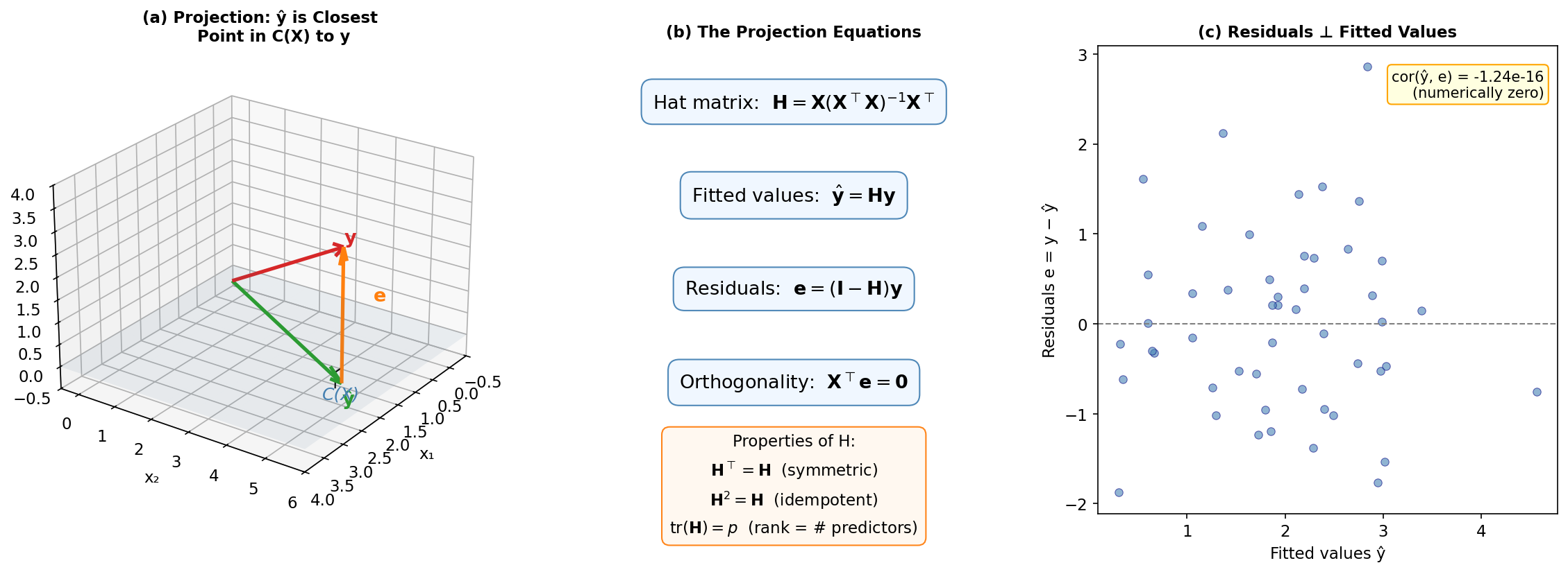
Fig. 256 Projection geometry in linear regression. (a) The response vector \(\mathbf{y}\) is projected onto the column space \(\mathcal{C}(\mathbf{X})\) to produce fitted values \(\hat{\mathbf{y}}\); the residual \(\mathbf{e}\) is perpendicular to the subspace. (b) The projection equations and hat matrix properties. (c) Numerical verification that residuals are orthogonal to fitted values.
Matrix Decompositions
Matrix decompositions reveal hidden structure. Each decomposition answers a different question about a matrix, and each has distinct computational applications.
Eigendecomposition (Spectral Decomposition)
Theorem: Spectral Theorem
Every real symmetric matrix \(\mathbf{A} \in \mathbb{R}^{n \times n}\) can be decomposed as:
where \(\mathbf{Q} = [\mathbf{q}_1 \mid \cdots \mid \mathbf{q}_n]\) is orthogonal (columns are the eigenvectors) and \(\boldsymbol{\Lambda} = \text{diag}(\lambda_1, \ldots, \lambda_n)\) contains the eigenvalues.
The eigendecomposition reveals:
Principal directions: The eigenvectors \(\mathbf{q}_i\) are the directions along which \(\mathbf{A}\) acts by pure scaling (no rotation)
Scaling factors: The eigenvalues \(\lambda_i\) give the scaling magnitude in each direction
Matrix functions: \(f(\mathbf{A}) = \mathbf{Q} \cdot \text{diag}(f(\lambda_1), \ldots, f(\lambda_n)) \cdot \mathbf{Q}^\top\), so \(\mathbf{A}^{-1} = \mathbf{Q}\boldsymbol{\Lambda}^{-1}\mathbf{Q}^\top\), \(\mathbf{A}^{1/2} = \mathbf{Q}\boldsymbol{\Lambda}^{1/2}\mathbf{Q}^\top\)
Definiteness: Read directly from the sign of eigenvalues
Markov convergence rate: For a stochastic matrix, the second-largest eigenvalue modulus \(|\lambda_2|\) governs how fast the chain converges to stationarity (see Section 5.4 Markov Chains: The Mathematical Foundation of MCMC)
import numpy as np

A = np.array([[4, 2],
               [2, 3]])

eigenvalues, Q = np.linalg.eigh(A)  # eigh for symmetric matrices
Lambda = np.diag(eigenvalues)

# Verify decomposition
print(f"Eigenvalues: {eigenvalues}")
print(f"Reconstruction error: {np.max(np.abs(A - Q @ Lambda @ Q.T)):.2e}")

# Matrix square root
A_sqrt = Q @ np.diag(np.sqrt(eigenvalues)) @ Q.T
print(f"(A^{1/2})^2 = A? {np.allclose(A_sqrt @ A_sqrt, A)}")  # True
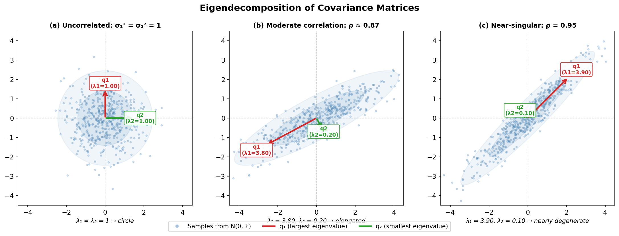
Fig. 257 Eigendecomposition of covariance matrices. The eigenvectors \(\mathbf{q}_1, \mathbf{q}_2\) give the principal directions of variation, and the eigenvalues \(\lambda_1, \lambda_2\) give the variance in each direction. As correlation increases from panel (a) to panel (c), the ellipse elongates and the smallest eigenvalue shrinks toward zero — the matrix approaches singularity.
Cholesky Decomposition
Theorem: Cholesky Decomposition
Every positive definite matrix \(\mathbf{A}\) has a unique decomposition:
where \(\mathbf{L}\) is lower triangular with positive diagonal entries. This is the Cholesky factor.
The Cholesky decomposition is the matrix analogue of taking a square root. It is:
Fast: \(O(n^3/3)\) operations — half the cost of a general LU factorization
Stable: Numerically well-conditioned for PD matrices
The PD test: If Cholesky fails, the matrix is not positive definite
Primary statistical application: Generating correlated random vectors. To sample \(\mathbf{X} \sim \mathcal{N}(\boldsymbol{\mu}, \boldsymbol{\Sigma})\):
Compute \(\mathbf{L}\) from \(\boldsymbol{\Sigma} = \mathbf{L}\mathbf{L}^\top\)
Generate \(\mathbf{Z} \sim \mathcal{N}(\mathbf{0}, \mathbf{I})\)
Set \(\mathbf{X} = \boldsymbol{\mu} + \mathbf{L}\mathbf{Z}\)
Then \(\text{Var}(\mathbf{X}) = \mathbf{L}\text{Var}(\mathbf{Z})\mathbf{L}^\top = \mathbf{L}\mathbf{I}\mathbf{L}^\top = \boldsymbol{\Sigma}\), using the variance rule for linear transformations (see Covariance Matrices below). This method is used throughout Section 2.4 Transformation Methods (Optional) for multivariate sampling.
Solving linear systems: To solve \(\mathbf{A}\mathbf{x} = \mathbf{b}\) with PD \(\mathbf{A}\), factor \(\mathbf{A} = \mathbf{L}\mathbf{L}^\top\), then solve the two triangular systems \(\mathbf{L}\mathbf{z} = \mathbf{b}\) (forward substitution) and \(\mathbf{L}^\top\mathbf{x} = \mathbf{z}\) (back substitution). Each triangular solve is \(O(n^2)\).
import numpy as np

Sigma = np.array([[1.0, 0.8, 0.3],
                   [0.8, 1.0, 0.5],
                   [0.3, 0.5, 1.0]])

L = np.linalg.cholesky(Sigma)
print(f"L =\n{L.round(4)}")
print(f"Reconstruction error: {np.max(np.abs(Sigma - L @ L.T)):.2e}")

# Generate correlated normals
rng = np.random.default_rng(42)
Z = rng.standard_normal((3, 10000))
X = L @ Z  # each column is a sample

print(f"Sample covariance:\n{np.cov(X).round(3)}")  # ≈ Sigma
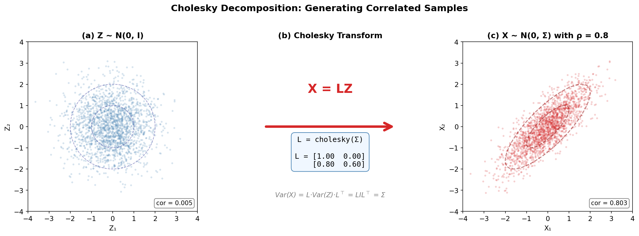
Fig. 258 Cholesky decomposition for generating correlated samples. (a) Independent standard normal draws \(\mathbf{Z} \sim \mathcal{N}(\mathbf{0}, \mathbf{I})\). (b) The Cholesky transform \(\mathbf{X} = \mathbf{L}\mathbf{Z}\) introduces the desired correlation structure. (c) The resulting samples \(\mathbf{X} \sim \mathcal{N}(\mathbf{0}, \boldsymbol{\Sigma})\) with \(\rho = 0.8\).
QR Decomposition
Theorem: QR Decomposition
Every matrix \(\mathbf{X} \in \mathbb{R}^{n \times p}\) with \(n \geq p\) and full column rank can be decomposed as:
where \(\mathbf{Q} \in \mathbb{R}^{n \times p}\) has orthonormal columns (\(\mathbf{Q}^\top\mathbf{Q} = \mathbf{I}_p\)) and \(\mathbf{R} \in \mathbb{R}^{p \times p}\) is upper triangular with positive diagonal entries.
The QR decomposition is the workhorse for numerically stable regression. Instead of forming \(\mathbf{X}^\top\mathbf{X}\) (which squares the condition number), substitute \(\mathbf{X} = \mathbf{Q}\mathbf{R}\) into the normal equations:
The last line is a triangular system — solved in \(O(p^2)\) by back-substitution. No matrix inversion needed.
The hat matrix simplifies to \(\mathbf{H} = \mathbf{Q}\mathbf{Q}^\top\), making leverage computation trivial: \(h_{ii} = \|\mathbf{q}_i\|^2\) where \(\mathbf{q}_i\) is the \(i\)-th row of \(\mathbf{Q}\).
import numpy as np

rng = np.random.default_rng(42)
n, p = 100, 5
X = rng.standard_normal((n, p))
y = X @ np.ones(p) + rng.standard_normal(n)

# QR-based regression (numerically stable)
Q, R = np.linalg.qr(X)
beta_qr = np.linalg.solve(R, Q.T @ y)

# Compare with direct normal equations (less stable)
beta_direct = np.linalg.solve(X.T @ X, X.T @ y)

print(f"Max difference: {np.max(np.abs(beta_qr - beta_direct)):.2e}")

# Leverage from Q
leverage_qr = np.sum(Q**2, axis=1)
H = X @ np.linalg.solve(X.T @ X, X.T)
leverage_direct = np.diag(H)
print(f"Leverage difference: {np.max(np.abs(leverage_qr - leverage_direct)):.2e}")
Singular Value Decomposition (SVD)
Theorem: Singular Value Decomposition
Every matrix \(\mathbf{X} \in \mathbb{R}^{n \times p}\) can be decomposed as:
where \(\mathbf{U} \in \mathbb{R}^{n \times n}\) and \(\mathbf{V} \in \mathbb{R}^{p \times p}\) are orthogonal, and \(\boldsymbol{\Sigma} \in \mathbb{R}^{n \times p}\) is “diagonal” with non-negative entries \(\sigma_1 \geq \sigma_2 \geq \cdots \geq \sigma_{\min(n,p)} \geq 0\) called the singular values.
The thin SVD (economical form) uses only the first \(r = \min(n, p)\) singular values: \(\mathbf{X} = \mathbf{U}_r \boldsymbol{\Sigma}_r \mathbf{V}_r^\top\).
The SVD is the most general decomposition — it applies to any matrix, not just square or PD ones. The singular values reveal the “energy” in each direction:
\(\sigma_i^2\) are the eigenvalues of \(\mathbf{X}^\top\mathbf{X}\) (the nonzero ones are also eigenvalues of \(\mathbf{X}\mathbf{X}^\top\))
Columns of \(\mathbf{V}\) are the right singular vectors (eigenvectors of \(\mathbf{X}^\top\mathbf{X}\))
Columns of \(\mathbf{U}\) are the left singular vectors (eigenvectors of \(\mathbf{X}\mathbf{X}^\top\))
Ridge regression via SVD: The ridge estimator \(\hat{\boldsymbol{\beta}}_\lambda = (\mathbf{X}^\top\mathbf{X} + \lambda\mathbf{I})^{-1}\mathbf{X}^\top\mathbf{y}\) becomes:
Along each singular direction, the OLS component is shrunk by the factor \(\sigma_i^2 / (\sigma_i^2 + \lambda)\). Directions with small singular values (near-collinear predictors) are shrunk the most — this is why ridge regression stabilizes ill-conditioned problems.
Effective degrees of freedom for ridge regression are \(\text{df}(\lambda) = \sum_i \sigma_i^2 / (\sigma_i^2 + \lambda)\), a smooth function that interpolates between \(p\) (at \(\lambda = 0\)) and \(0\) (as \(\lambda \to \infty\)). See Section 4.8: Cross-Validation Methods (Optional).
Condition number: \(\kappa(\mathbf{X}) = \sigma_1 / \sigma_p\). A large condition number means the matrix is nearly singular — small perturbations in the data cause large changes in the solution. When \(\kappa \gg 1\), use QR or SVD rather than forming \(\mathbf{X}^\top\mathbf{X}\).
import numpy as np

rng = np.random.default_rng(42)
n, p = 100, 5
X = rng.standard_normal((n, p))

U, sigma, Vt = np.linalg.svd(X, full_matrices=False)
print(f"Singular values: {sigma.round(3)}")
print(f"Condition number: {sigma[0] / sigma[-1]:.2f}")

# Ridge regression via SVD
y = X @ np.ones(p) + rng.standard_normal(n)
lam = 1.0
d = sigma / (sigma**2 + lam)  # multiplies U.T @ y; shrinkage factor is sigma**2/(sigma**2 + lam)
beta_ridge = Vt.T @ (d * (U.T @ y))

# Effective degrees of freedom
df_ridge = np.sum(sigma**2 / (sigma**2 + lam))
print(f"Effective df: {df_ridge:.2f}")  # < p = 5
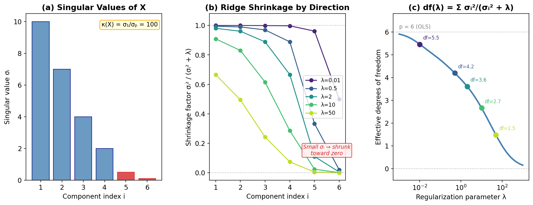
Fig. 259 SVD and ridge regression shrinkage. (a) Singular values of the design matrix — small values (red) indicate near-collinear directions. (b) Ridge shrinkage factors \(\sigma_i^2/(\sigma_i^2 + \lambda)\) by SVD component: weak directions are shrunk most aggressively. (c) Effective degrees of freedom decrease smoothly from \(p\) to 0 as regularization \(\lambda\) increases.
The SVD view explains how much ridge shrinks each direction. There is a complementary geometric picture of where the regularized solution lands: the penalty defines a constraint region in coefficient space, and the solution is the first point where the expanding RSS contours touch that region. The shape of the region — the smooth \(L_2\) disk of ridge versus the cornered \(L_1\) diamond of the LASSO — determines whether coefficients merely shrink or are set exactly to zero.
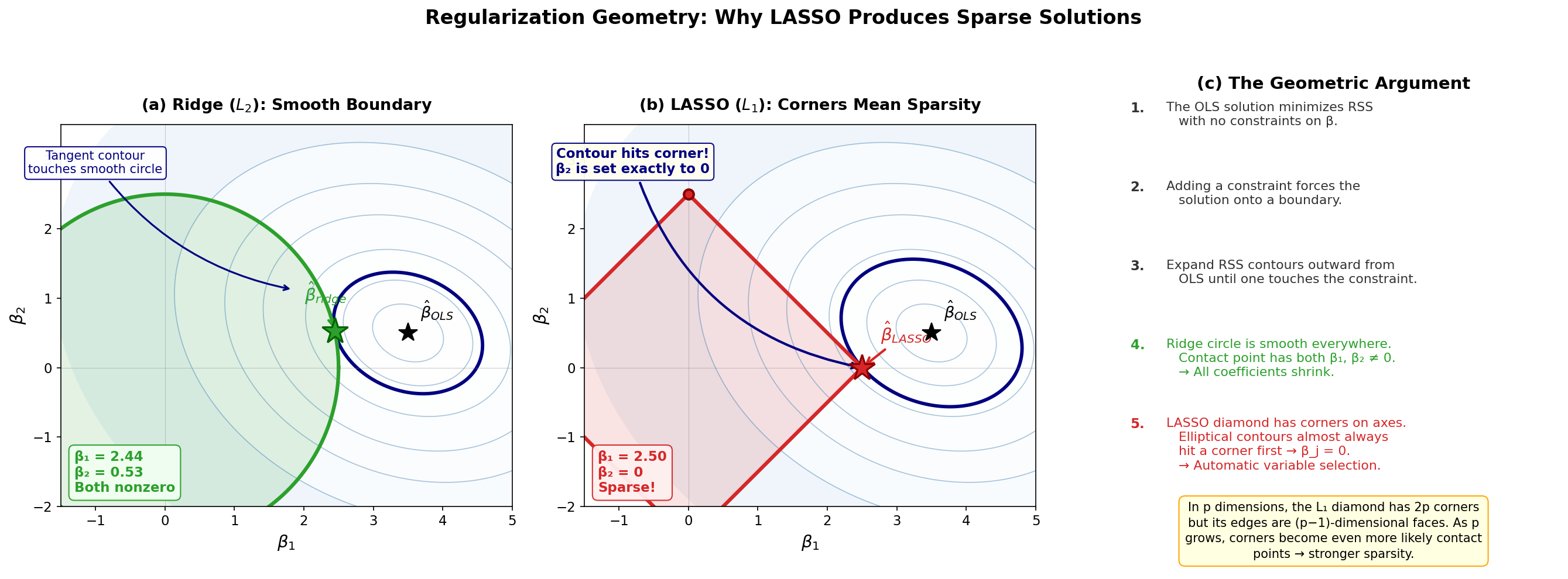
Fig. 260 Regularization geometry: Ridge vs LASSO. RSS contour ellipses expand outward from the unconstrained OLS solution until they touch the constraint region. (a) The \(L_2\) circle (Ridge) has a smooth boundary, so the tangent point has both \(\beta_1, \beta_2 \neq 0\). (b) The \(L_1\) diamond (LASSO) has corners on the coordinate axes; the first contour to touch the diamond typically hits a corner where \(\beta_j = 0\), producing a sparse solution. (c) The geometric argument summarized step by step, with a note on higher dimensions: the \(L_1\) ball in \(p\) dimensions has \(2p\) corners, so corner contact — and hence automatic variable selection — becomes even more likely as \(p\) grows.
Decomposition Summary
Decomposition |
Requirements |
Cost |
Primary Use in This Course |
|---|---|---|---|
Eigen (\(\mathbf{Q}\boldsymbol{\Lambda}\mathbf{Q}^\top\)) |
Symmetric |
\(O(n^3)\) |
PCA, Markov chain convergence, definiteness tests |
Cholesky (\(\mathbf{L}\mathbf{L}^\top\)) |
Symmetric PD |
\(O(n^3/3)\) |
Sampling correlated normals, solving PD systems |
QR (\(\mathbf{Q}\mathbf{R}\)) |
Full column rank |
\(O(2np^2)\) for thin QR |
Numerically stable regression, leverage |
SVD (\(\mathbf{U}\boldsymbol{\Sigma}\mathbf{V}^\top\)) |
Any matrix |
\(O(\min(mn^2, m^2n))\) |
Ridge regression, condition number, rank determination |
Quadratic Forms and Covariance
Quadratic forms — expressions of the form \(\mathbf{x}^\top\mathbf{A}\mathbf{x}\) — are ubiquitous in statistics. They appear in the multivariate normal density, in sum-of-squares decompositions, in the chi-square distribution, and in every optimization problem involving least squares.
Quadratic Forms
For a symmetric matrix \(\mathbf{A} \in \mathbb{R}^{n \times n}\) and vector \(\mathbf{x} \in \mathbb{R}^n\):
The sign behavior of \(Q\) is determined by the definiteness of \(\mathbf{A}\):
\(\mathbf{A}\) positive definite \(\Rightarrow Q(\mathbf{x}) > 0\) for all \(\mathbf{x} \neq \mathbf{0}\) (bowl opening upward)
\(\mathbf{A}\) negative definite \(\Rightarrow Q(\mathbf{x}) < 0\) for all \(\mathbf{x} \neq \mathbf{0}\) (bowl opening downward)
\(\mathbf{A}\) indefinite \(\Rightarrow Q\) takes both positive and negative values (saddle)
Statistical connection: The Mahalanobis distance \((\mathbf{x} - \boldsymbol{\mu})^\top \boldsymbol{\Sigma}^{-1} (\mathbf{x} - \boldsymbol{\mu})\) in the multivariate normal density is a quadratic form in \(\boldsymbol{\Sigma}^{-1}\). Its level sets are ellipsoids whose axes align with the eigenvectors of \(\boldsymbol{\Sigma}\).
Chi-square connection: If \(\mathbf{Z} \sim \mathcal{N}(\mathbf{0}, \mathbf{I}_p)\), then \(\mathbf{Z}^\top\mathbf{Z} = \sum_{i=1}^p Z_i^2 \sim \chi^2_p\). More generally, if \(\mathbf{P}\) is a symmetric idempotent matrix of rank \(r\), then \(\mathbf{Z}^\top\mathbf{P}\mathbf{Z} \sim \chi^2_r\). This is the basis for the chi-square distribution of RSS/\(\sigma^2\) in linear models.
Covariance Matrices
Definition
The covariance matrix of a random vector \(\mathbf{X} = (X_1, \ldots, X_p)^\top\) is:
where \(\Sigma_{ij} = \text{Cov}(X_i, X_j)\) and \(\boldsymbol{\mu} = \mathbb{E}[\mathbf{X}]\).
Every covariance matrix is symmetric and positive semi-definite (PSD). It is PD if and only if no component is a deterministic linear combination of others.
Variance of linear combinations. For a constant matrix \(\mathbf{A}\) and random vector \(\mathbf{X}\):
This formula propagates uncertainty through linear transformations and is the matrix foundation for:
The variance of the OLS estimator: \(\text{Var}(\hat{\boldsymbol{\beta}}) = \sigma^2 (\mathbf{X}^\top\mathbf{X})^{-1}\)
The sandwich estimator for robust variance: \((\mathbf{X}^\top\mathbf{X})^{-1}\mathbf{X}^\top\text{diag}(e_i^2)\mathbf{X}(\mathbf{X}^\top\mathbf{X})^{-1}\)
The multivariate delta method: \(\text{Var}(g(\hat{\boldsymbol{\theta}})) \approx \mathbf{J} \text{Var}(\hat{\boldsymbol{\theta}}) \mathbf{J}^\top\)
Derivation: Variance of OLS Estimator
Under the model \(\mathbf{y} = \mathbf{X}\boldsymbol{\beta} + \boldsymbol{\varepsilon}\) with \(\text{Var}(\boldsymbol{\varepsilon}) = \sigma^2 \mathbf{I}\):
using the \(\text{Var}(\mathbf{A}\mathbf{X}) = \mathbf{A}\text{Var}(\mathbf{X})\mathbf{A}^\top\) rule with \(\mathbf{A} = (\mathbf{X}^\top\mathbf{X})^{-1}\mathbf{X}^\top\).
import numpy as np

rng = np.random.default_rng(42)
n, p = 1000, 3
true_beta = np.array([1, 2, -1])
sigma = 0.5

X = rng.standard_normal((n, p))
y = X @ true_beta + sigma * rng.standard_normal(n)

# OLS and its variance
XtX_inv = np.linalg.inv(X.T @ X)
beta_hat = XtX_inv @ X.T @ y
s2 = np.sum((y - X @ beta_hat)**2) / (n - p)
var_beta = s2 * XtX_inv

print(f"Estimated beta: {beta_hat.round(4)}")
print(f"Standard errors: {np.sqrt(np.diag(var_beta)).round(4)}")
Matrix Calculus
Optimization-based inference — MLE, MAP estimation, Fisher scoring — requires taking derivatives of scalar functions with respect to vectors and matrices. Matrix calculus provides compact notation for these operations.
Gradients of Scalar Functions
For a scalar-valued function \(f: \mathbb{R}^p \to \mathbb{R}\), the gradient is the column vector of partial derivatives:
The gradient points in the direction of steepest ascent. Setting \(\nabla f = \mathbf{0}\) finds critical points — the basis for all optimization-based estimation.
Key gradient identities (for constant \(\mathbf{a}\), \(\mathbf{b}\), and symmetric \(\mathbf{A}\)):
Derivation: Gradient of a Quadratic Form
For symmetric \(\mathbf{A}\), write out \(f(\mathbf{x}) = \mathbf{x}^\top\mathbf{A}\mathbf{x} = \sum_i \sum_j A_{ij} x_i x_j\). Then:
where the last equality uses \(A_{ik} = A_{ki}\) (symmetry). In matrix notation, this is \(2\mathbf{A}\mathbf{x}\).
The Hessian Matrix
The Hessian is the matrix of second partial derivatives:
The Hessian is always symmetric (by equality of mixed partials for smooth functions). At a critical point \(\boldsymbol{\theta}^*\):
\(\mathbf{H}\) negative definite \(\Rightarrow\) local maximum (used to verify MLEs)
\(\mathbf{H}\) positive definite \(\Rightarrow\) local minimum
In MLE, the observed Fisher information is \(\mathbf{J}(\hat{\boldsymbol{\theta}}) = -\mathbf{H}_\ell(\hat{\boldsymbol{\theta}})\) — the negative Hessian of the log-likelihood evaluated at the MLE. Its inverse estimates the covariance of \(\hat{\boldsymbol{\theta}}\) (see Section 3.2 Maximum Likelihood Estimation).
Derivative of Log-Determinant
For a positive definite matrix \(\mathbf{A}(\boldsymbol{\theta})\) that depends on parameters:
This identity appears in ML estimation for linear models (differentiating the normal log-likelihood with respect to variance parameters) and in computing the Fisher information for multivariate models.
Jacobian and Change of Variables
Definition
The Jacobian matrix of a vector-valued function \(\mathbf{g}: \mathbb{R}^p \to \mathbb{R}^q\) is:
The Jacobian plays two roles in this course:
Change of variables in densities: If \(\mathbf{Y} = \mathbf{g}(\mathbf{X})\) where \(\mathbf{g}\) is a bijection, then:
\[f_{\mathbf{Y}}(\mathbf{y}) = f_{\mathbf{X}}(\mathbf{g}^{-1}(\mathbf{y})) \cdot \left|\det \mathbf{J}_{\mathbf{g}^{-1}}(\mathbf{y})\right|\]This is essential for deriving distributions of transformed random vectors (see Section 2.4 Transformation Methods (Optional)) and for constructing Jeffreys priors under reparameterization (see Section 5.2 Prior Specification and Conjugate Analysis).
Multivariate delta method: For an estimator \(\hat{\boldsymbol{\theta}} \xrightarrow{d} \mathcal{N}(\boldsymbol{\theta}, \boldsymbol{\Sigma}/n)\) and a smooth function \(\mathbf{g}\):
\[\mathbf{g}(\hat{\boldsymbol{\theta}}) \xrightarrow{d} \mathcal{N}\!\left(\mathbf{g}(\boldsymbol{\theta}),\; \mathbf{J}_{\mathbf{g}}(\boldsymbol{\theta}) \frac{\boldsymbol{\Sigma}}{n} \mathbf{J}_{\mathbf{g}}(\boldsymbol{\theta})^\top\right)\]See Section 3.3 Sampling Variability and Variance Estimation for the full development.
Numerical Considerations
The formulas in this appendix are exact in real arithmetic, but computers compute in finite-precision floating point, where mathematically equivalent algorithms can differ enormously in accuracy. This section introduces the condition number — the standard measure of how much a problem amplifies small errors — and the practical rules it implies for statistical computation.
Condition Number and Stability
The condition number of a matrix \(\mathbf{A}\) measures how sensitive the solution of \(\mathbf{A}\mathbf{x} = \mathbf{b}\) is to perturbations in \(\mathbf{A}\) or \(\mathbf{b}\):
where \(\sigma_{\max}\) and \(\sigma_{\min}\) are the largest and smallest singular values. A relative perturbation of size \(\epsilon\) in the data can cause a relative perturbation of up to \(\kappa \cdot \epsilon\) in the solution.
Rules of thumb:
\(\kappa \approx 1\): Well-conditioned (orthogonal matrices have \(\kappa = 1\))
\(\kappa \approx 10^k\): Expect to lose about \(k\) digits of accuracy
\(\kappa > 10^{15}\): Effectively singular in double precision (\(\approx 16\) digits)
When \(\kappa(\mathbf{X})\) is large (due to near-collinear predictors), forming \(\mathbf{X}^\top\mathbf{X}\) squares the condition number to \(\kappa^2\) — potentially catastrophic (see Appendix C for how floating-point precision and condition numbers interact to determine digits of accuracy lost). This is why numerical linear algebra avoids \(\mathbf{X}^\top\mathbf{X}\) and instead uses QR or SVD.
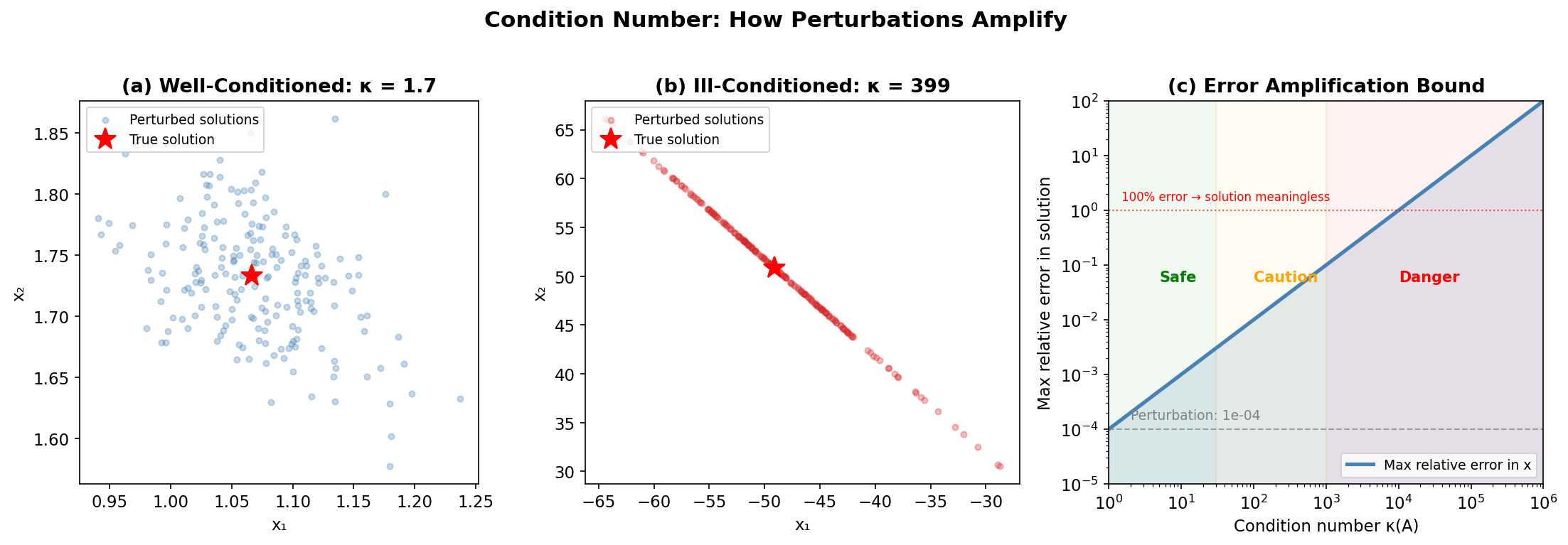
Fig. 261 Condition number and perturbation sensitivity. (a) A well-conditioned system: small perturbations in \(\mathbf{b}\) cause small changes in the solution. (b) An ill-conditioned system: the same perturbations cause the solution to scatter wildly. (c) The error amplification bound: the condition number \(\kappa\) multiplies input perturbations to give the worst-case output error.
Avoiding \(\mathbf{X}^\top\mathbf{X}\)
The following operations should use decompositions rather than forming \(\mathbf{X}^\top\mathbf{X}\) explicitly:
Task |
Naive (Avoid) |
Stable (Prefer) |
|---|---|---|
Solve \(\mathbf{X}^\top\mathbf{X}\boldsymbol{\beta} = \mathbf{X}^\top\mathbf{y}\) |
|
|
Compute leverage \(h_{ii}\) |
|
|
Solve PD system \(\mathbf{A}\mathbf{x} = \mathbf{b}\) |
|
|
Near-Singular Matrices
When a covariance matrix is theoretically PD but numerically near-singular (e.g., due to highly correlated variables or limited floating-point precision), the Cholesky decomposition may fail. Common remedies:
Jitter: Add a small multiple of the identity: \(\boldsymbol{\Sigma} + \epsilon \mathbf{I}\) with \(\epsilon \sim 10^{-6}\). This nudges all eigenvalues away from zero.
Regularization: Use ridge-type shrinkage toward the identity: \((1-\alpha)\boldsymbol{\Sigma} + \alpha \mathbf{I}\)
Pivoted Cholesky: Detects and handles rank deficiency gracefully
import numpy as np

# Ill-conditioned design matrix
rng = np.random.default_rng(42)
X = rng.standard_normal((100, 5))
X[:, 4] = X[:, 3] + 1e-8 * rng.standard_normal(100)  # nearly collinear

print(f"Condition number of X: {np.linalg.cond(X):.2e}")
print(f"Condition number of X'X: {np.linalg.cond(X.T @ X):.2e}")  # squared!

# QR is stable even here
Q, R = np.linalg.qr(X)
y = rng.standard_normal(100)
beta = np.linalg.solve(R, Q.T @ y)  # works fine
Key Takeaways
Key Takeaways 📝
Matrices are linear transformations, not just arrays of numbers. Reading \(\mathbf{H}\mathbf{y}\) as “project \(\mathbf{y}\) onto the column space” is more useful than computing entry by entry.
Special structure enables shortcuts: Symmetric → real eigenvalues; PD → Cholesky; idempotent → eigenvalues in {0,1}; block diagonal → invert each block independently.
Block matrix algebra (Schur complement, Sherman-Morrison-Woodbury) turns expensive \(n \times n\) problems into cheaper \(k \times k\) problems when structure is present.
Decompositions reveal structure: Eigen shows principal directions; Cholesky enables sampling; QR gives numerical stability; SVD handles everything else (rank, condition, regularization).
Variance propagates through linear transformations by \(\text{Var}(\mathbf{A}\mathbf{X}) = \mathbf{A}\text{Var}(\mathbf{X})\mathbf{A}^\top\) — the single rule behind the OLS variance \(\sigma^2(\mathbf{X}^\top\mathbf{X})^{-1}\), the delta method, and Cholesky-based sampling of correlated normals.
Never form \(\mathbf{X}^\top\mathbf{X}\) when you can avoid it. Use QR or SVD for regression. Use
solveinstead ofinv. Use Cholesky for PD systems. The algorithms are faster and more accurate.Matrix calculus is the language of multivariate optimization: the gradient finds critical points, the Hessian classifies them, and the Jacobian propagates uncertainty through transformations.
Looking Ahead
The linear algebra developed here supports multiple threads in the main course:
Chapters 3-4: The hat matrix, projection geometry, QR decomposition, and Sherman-Morrison-Woodbury formula are the computational backbone of linear models, influence diagnostics, and cross-validation shortcuts.
Chapter 5: Stochastic matrices and eigendecomposition govern Markov chain convergence, Cholesky decomposition enables correlated proposals in MCMC, and the mass matrix in HMC is a covariance-scaled inner product.
Throughout: Matrix calculus (gradients, Hessians, Jacobians) is the shared language of Fisher information, Newton-Raphson optimization, the delta method, and automatic differentiation.
Practice Problems
These exercises connect the linear algebra concepts from this appendix to their statistical applications, combining mathematical derivations with computational verification.
Exercise 1: Projection Geometry and the Hat Matrix
In linear regression, the hat matrix \(\mathbf{H} = \mathbf{X}(\mathbf{X}^\top\mathbf{X})^{-1}\mathbf{X}^\top\) projects the response vector onto the column space of \(\mathbf{X}\). This exercise explores its geometric and statistical properties.
Given a design matrix \(\mathbf{X}\) (\(n=50\), \(p=3\) with intercept + 2 predictors), compute \(\mathbf{H} = \mathbf{X}(\mathbf{X}^\top\mathbf{X})^{-1}\mathbf{X}^\top\). Prove mathematically that \(\mathbf{H}\) is symmetric and idempotent, then verify computationally.
Hint: Symmetry and Idempotency
For symmetry, take the transpose and use \((\mathbf{A}\mathbf{B})^\top = \mathbf{B}^\top\mathbf{A}^\top\). For idempotency, expand \(\mathbf{H}^2\) and simplify using the fact that \((\mathbf{X}^\top\mathbf{X})^{-1}\mathbf{X}^\top\mathbf{X} = \mathbf{I}\).
Show that the diagonal entries \(h_{ii}\) (leverage values) satisfy \(1/n \leq h_{ii} \leq 1\), and that they sum to \(p\). Compute leverage for your \(\mathbf{X}\) and identify the highest-leverage observation. Explain geometrically why leverage measures “distance from the center of predictor space.”
Hint: Leverage Bounds
\(h_{ii} = \mathbf{x}_i^\top(\mathbf{X}^\top\mathbf{X})^{-1}\mathbf{x}_i\) is a quadratic form. The bounds come from \(\mathbf{H}\) being idempotent (eigenvalues 0 or 1) and the trace equaling \(p\). Since \(\text{tr}(\mathbf{H}) = p\) and \(0 \leq h_{ii} \leq 1\), the average leverage is \(p/n\).
Add an outlier at a high-leverage point: set one observation’s predictors to extreme values and its response to an unusual value. Show how the hat matrix concentrates influence — compare the fitted value at the outlier with and without using the hat matrix to quantify how much the outlier “pulls” the fit toward itself.
Hint: Influence at High-Leverage Points
For a high-leverage point, \(h_{ii}\) is close to 1, meaning \(\hat{y}_i \approx y_i\) — the fit is forced through that point regardless of the other data. This is because \(\hat{y}_i = h_{ii} y_i + \sum_{j \neq i} h_{ij} y_j\), and when \(h_{ii} \approx 1\), the first term dominates.
Verify the fundamental orthogonality: \(\mathbf{X}^\top\mathbf{e} = \mathbf{0}\) where \(\mathbf{e} = (\mathbf{I} - \mathbf{H})\mathbf{y}\). Interpret geometrically: the residual vector is perpendicular to every column of \(\mathbf{X}\).
Hint: Orthogonality of Residuals
Expand \(\mathbf{X}^\top\mathbf{e} = \mathbf{X}^\top(\mathbf{I} - \mathbf{H})\mathbf{y} = \mathbf{X}^\top\mathbf{y} - \mathbf{X}^\top\mathbf{H}\mathbf{y}\). Then substitute \(\mathbf{H} = \mathbf{X}(\mathbf{X}^\top\mathbf{X})^{-1}\mathbf{X}^\top\) and simplify: \(\mathbf{X}^\top\mathbf{H} = \mathbf{X}^\top\mathbf{X}(\mathbf{X}^\top\mathbf{X})^{-1}\mathbf{X}^\top = \mathbf{X}^\top\).
Solution
Part (a): Symmetry and Idempotency — Mathematical Proof
Symmetry:
where we used \((\mathbf{X}^\top\mathbf{X})^\top = \mathbf{X}^\top\mathbf{X}\) (symmetric matrix) and \((\mathbf{A}^{-1})^\top = (\mathbf{A}^\top)^{-1}\).
Idempotency:
Computational Verification:
import numpy as np

rng = np.random.default_rng(seed=42)

# Design matrix: intercept + 2 predictors, n=50, p=3
n, p = 50, 3
X = np.column_stack([
    np.ones(n),
    rng.standard_normal(n),
    rng.standard_normal(n)
])

# Hat matrix
H = X @ np.linalg.solve(X.T @ X, X.T)

# Verify symmetry: H = H^T
sym_error = np.max(np.abs(H - H.T))
print(f"Symmetry check: max|H - H^T| = {sym_error:.2e}")

# Verify idempotency: H^2 = H
idem_error = np.max(np.abs(H @ H - H))
print(f"Idempotency check: max|H^2 - H| = {idem_error:.2e}")

# Eigenvalues should be 0 or 1
eigvals = np.linalg.eigvalsh(H)
print(f"\nEigenvalues of H (sorted):")
print(f"  Number near 0: {np.sum(np.abs(eigvals) < 1e-10)}")
print(f"  Number near 1: {np.sum(np.abs(eigvals - 1) < 1e-10)}")
print(f"  Trace(H) = sum of eigenvalues = {np.trace(H):.6f} (should be p={p})")
Symmetry check: max|H - H^T| = 2.78e-17
Idempotency check: max|H^2 - H| = 4.16e-17

Eigenvalues of H (sorted):
  Number near 0: 47
  Number near 1: 3
  Trace(H) = sum of eigenvalues = 3.000000 (should be p=3)
Part (b): Leverage Values
Since \(\text{tr}(\mathbf{H}) = p\) and \(\mathbf{H}\) is idempotent with eigenvalues in \(\{0, 1\}\), each diagonal satisfies \(0 \leq h_{ii} \leq 1\). When \(\mathbf{X}\) includes an intercept column, we additionally have \(h_{ii} \geq 1/n\) because the intercept contribution alone gives \(1/n\).
import numpy as np

rng = np.random.default_rng(seed=42)

n, p = 50, 3
X = np.column_stack([
    np.ones(n),
    rng.standard_normal(n),
    rng.standard_normal(n)
])

H = X @ np.linalg.solve(X.T @ X, X.T)
leverages = np.diag(H)

print(f"Leverage statistics:")
print(f"  Sum of leverages: {np.sum(leverages):.6f} (should be p={p})")
print(f"  Mean leverage: {np.mean(leverages):.6f} (should be p/n={p/n:.4f})")
print(f"  Min leverage: {np.min(leverages):.6f} (lower bound 1/n={1/n:.4f})")
print(f"  Max leverage: {np.max(leverages):.6f} (upper bound 1)")
print(f"\nHighest-leverage observation:")
i_max = np.argmax(leverages)
print(f"  Index: {i_max}")
print(f"  Leverage h_ii: {leverages[i_max]:.6f}")
print(f"  Predictor values: x1={X[i_max, 1]:.4f}, x2={X[i_max, 2]:.4f}")
print(f"  Distance from predictor centroid: {np.sqrt(np.sum((X[i_max, 1:] - X[:, 1:].mean(axis=0))**2)):.4f}")
Leverage statistics:
  Sum of leverages: 3.000000 (should be p=3)
  Mean leverage: 0.060000 (should be p/n=0.0600)
  Min leverage: 0.020281 (lower bound 1/n=0.0200)
  Max leverage: 0.183434 (upper bound 1)

Highest-leverage observation:
  Index: 30
  Leverage h_ii: 0.183434
  Predictor values: x1=2.1416, x2=0.4568
  Distance from predictor centroid: 2.1506
The highest-leverage point is the one farthest from the centroid of the predictor space, confirming the geometric interpretation: leverage measures how “unusual” an observation’s predictor values are.
Part (c): Outlier at a High-Leverage Point
import numpy as np

rng = np.random.default_rng(seed=42)

n, p = 50, 3
X = np.column_stack([
    np.ones(n),
    rng.standard_normal(n),
    rng.standard_normal(n)
])
beta_true = np.array([2.0, -1.5, 0.8])
y = X @ beta_true + 0.5 * rng.standard_normal(n)

# Create a high-leverage outlier: extreme predictor values, unusual response
X_outlier = X.copy()
y_outlier = y.copy()
X_outlier[0, 1] = 8.0   # Far from center
X_outlier[0, 2] = 8.0
y_outlier[0] = 50.0     # Unusual response

# Compute hat matrix with the outlier
H_out = X_outlier @ np.linalg.solve(X_outlier.T @ X_outlier, X_outlier.T)
leverages_out = np.diag(H_out)

print(f"Leverage of outlier point: h_00 = {leverages_out[0]:.6f}")
print(f"Next highest leverage: {np.sort(leverages_out)[-2]:.6f}")

# Fitted values
beta_hat = np.linalg.solve(X_outlier.T @ X_outlier, X_outlier.T @ y_outlier)
y_hat = X_outlier @ beta_hat

print(f"\nOutlier: y_0 = {y_outlier[0]:.2f}, y_hat_0 = {y_hat[0]:.4f}")
print(f"Ratio y_hat_0 / y_0 = {y_hat[0] / y_outlier[0]:.4f}")
print(f"h_00 = {leverages_out[0]:.4f} (close to ratio above)")
print(f"\nInterpretation: since h_00 ≈ {leverages_out[0]:.3f}, the fit is")
print(f"forced {100*leverages_out[0]:.1f}% of the way toward the outlier's y-value.")
Leverage of outlier point: h_00 = 0.825435
Next highest leverage: 0.109281

Outlier: y_0 = 50.00, y_hat_0 = 40.8597
Ratio y_hat_0 / y_0 = 0.8172
h_00 = 0.8254 (close to ratio above)

Interpretation: since h_00 ≈ 0.825, the fit is
forced 82.5% of the way toward the outlier's y-value.
With \(h_{ii} \approx 0.83\), the regression is forced mostly through the outlier regardless of the other 49 observations. This is the danger of high-leverage points: they can dominate the fit.
Part (d): Orthogonality of Residuals
Proof: \(\mathbf{X}^\top\mathbf{e} = \mathbf{X}^\top(\mathbf{I} - \mathbf{H})\mathbf{y} = \mathbf{X}^\top\mathbf{y} - \mathbf{X}^\top\mathbf{H}\mathbf{y}\).
Substituting \(\mathbf{H}\):
Therefore \(\mathbf{X}^\top\mathbf{e} = \mathbf{X}^\top\mathbf{y} - \mathbf{X}^\top\mathbf{y} = \mathbf{0}\).
Geometric interpretation: The residual vector \(\mathbf{e}\) lives in the orthogonal complement of \(\text{col}(\mathbf{X})\). It is perpendicular to every column of \(\mathbf{X}\), including the intercept column (which forces \(\sum e_i = 0\)).
import numpy as np

rng = np.random.default_rng(seed=42)

n, p = 50, 3
X = np.column_stack([
    np.ones(n),
    rng.standard_normal(n),
    rng.standard_normal(n)
])
beta_true = np.array([2.0, -1.5, 0.8])
y = X @ beta_true + 0.5 * rng.standard_normal(n)

# Compute hat matrix and residuals
H = X @ np.linalg.solve(X.T @ X, X.T)
y_hat = H @ y
e = y - y_hat  # equivalently, (I - H) @ y

# Verify orthogonality
ortho_check = X.T @ e
print("X^T @ e (should be zero vector):")
print(f"  {ortho_check}")
print(f"  Max absolute value: {np.max(np.abs(ortho_check)):.2e}")

# Consequence: residuals sum to zero (orthogonal to intercept column)
print(f"\nSum of residuals: {np.sum(e):.2e} (orthogonal to ones column)")
print(f"Correlation of residuals with x1: {np.corrcoef(X[:, 1], e)[0, 1]:.2e}")
print(f"Correlation of residuals with x2: {np.corrcoef(X[:, 2], e)[0, 1]:.2e}")
X^T @ e (should be zero vector):
  [ 4.44089210e-15 -1.50920942e-15  2.66453526e-15]
  Max absolute value: 4.44e-15

Sum of residuals: 4.44e-15 (orthogonal to ones column)
Correlation of residuals with x1: -9.63e-17
Correlation of residuals with x2: 1.95e-16
The residuals are orthogonal to the column space of \(\mathbf{X}\) to machine precision, confirming the projection geometry.
Exercise 2: Matrix Decompositions for Ill-Conditioned Regression
When predictors are nearly collinear, the normal equations become numerically unstable. This exercise compares decomposition-based approaches and introduces ridge regularization through the SVD lens.
Create an ill-conditioned design matrix: generate \(\mathbf{X}\) (\(n=100\), \(p=5\)) with
rng.standard_normal, then setX[:,4] = X[:,3] + 1e-6 * rng.standard_normal(100)to create near-collinearity. Compute \(\kappa(\mathbf{X})\) and \(\kappa(\mathbf{X}^\top\mathbf{X})\) and verify the squaring relationship.Hint: Condition Number Squaring
np.linalg.cond()computes the condition number. For well-conditioned \(\mathbf{X}\), \(\kappa(\mathbf{X}^\top\mathbf{X}) \approx \kappa(\mathbf{X})^2\). This is because the singular values of \(\mathbf{X}^\top\mathbf{X}\) are the squares of the singular values of \(\mathbf{X}\).Generate \(\mathbf{y} = \mathbf{X}\boldsymbol{\beta} + \boldsymbol{\varepsilon}\) with known \(\boldsymbol{\beta} = [1, -2, 1.5, 0.5, -0.3]^\top\) and solve OLS three ways: (1) Normal equations via
np.linalg.inv(X.T @ X) @ X.T @ y, (2) QR decomposition, (3)np.linalg.lstsq. Compare the solutions — does any method recover \(\boldsymbol{\beta}\) accurately? Explain why not.Hint: QR Solution Method
For QR, factor \(\mathbf{X} = \mathbf{Q}\mathbf{R}\), then \(\hat{\boldsymbol{\beta}} = \mathbf{R}^{-1}\mathbf{Q}^\top\mathbf{y}\) via
np.linalg.solve(R, Q.T @ y).lstsquses SVD internally and is the most robust.Apply ridge regression via the SVD: compute \(\mathbf{X} = \mathbf{U}\boldsymbol{\Sigma}\mathbf{V}^\top\) and show that \(\hat{\boldsymbol{\beta}}_{\text{ridge}} = \mathbf{V} \text{diag}\left(\frac{\sigma_i}{\sigma_i^2 + \lambda}\right) \mathbf{U}^\top\mathbf{y}\). For \(\lambda \in \{0.001, 0.1, 1, 10\}\), compute the shrinkage factors and effective degrees of freedom \(\text{df}(\lambda) = \sum_i \frac{\sigma_i^2}{\sigma_i^2 + \lambda}\).
Hint: SVD Shrinkage Geometry
Small singular values (the near-collinear directions) get shrunk most aggressively. This is the geometric insight: ridge regression stabilizes by damping the directions where \(\mathbf{X}\) has little information. The shrinkage factor \(\sigma_i^2 / (\sigma_i^2 + \lambda)\) is near 1 for large \(\sigma_i\) and near 0 for small \(\sigma_i\).
Demonstrate the Cholesky speed advantage: for a \(500 \times 500\) positive definite matrix, time
scipy.linalg.solve(A, b)(general LU-based) vsscipy.linalg.cho_solve(scipy.linalg.cho_factor(A), b). For solving multiple right-hand sides (e.g., 100), show that Cholesky factorize-once-solve-many is faster.Hint: Cholesky Factorize-Once Strategy
Use
import timefor simple timing.cho_factorcomputes \(\mathbf{L}\) once;cho_solvereuses it for each \(\mathbf{b}\). The advantage grows with the number of right-hand sides because the \(O(n^3)\) factorization is done once rather than repeatedly.
Solution
Part (a): Condition Number and the Squaring Relationship
import numpy as np

rng = np.random.default_rng(seed=42)

n, p = 100, 5
X = rng.standard_normal((n, p))

# Create near-collinearity: column 4 ≈ column 3
X[:, 4] = X[:, 3] + 1e-6 * rng.standard_normal(n)

cond_X = np.linalg.cond(X)
cond_XtX = np.linalg.cond(X.T @ X)

print(f"Condition number of X: κ(X) = {cond_X:.4e}")
print(f"Condition number of X'X: κ(X'X) = {cond_XtX:.4e}")
print(f"κ(X)^2 = {cond_X**2:.4e}")
print(f"Ratio κ(X'X) / κ(X)^2 = {cond_XtX / cond_X**2:.6f}")
print(f"\nSingular values of X:")
svs = np.linalg.svd(X, compute_uv=False)
for i, sv in enumerate(svs):
    print(f"  σ_{i+1} = {sv:.6f}")
print(f"\nRatio σ_max/σ_min = {svs[0]/svs[-1]:.4e} = κ(X)")
Condition number of X: κ(X) = 2.0454e+06
Condition number of X'X: κ(X'X) = 4.1796e+12
κ(X)^2 = 4.1835e+12
Ratio κ(X'X) / κ(X)^2 = 0.999065

Singular values of X:
  σ_1 = 14.964792
  σ_2 = 9.966658
  σ_3 = 9.128724
  σ_4 = 8.244767
  σ_5 = 0.000007

Ratio σ_max/σ_min = 2.0454e+06 = κ(X)
The near-collinearity creates one tiny singular value (\(\sigma_5 \approx 7 \times 10^{-6}\)), making \(\kappa(\mathbf{X}) \approx 2 \times 10^6\). The squaring relationship \(\kappa(\mathbf{X}^\top\mathbf{X}) \approx \kappa(\mathbf{X})^2\) holds because the singular values of \(\mathbf{X}^\top\mathbf{X}\) are \(\sigma_i^2\).
Part (b): Three OLS Methods Compared
import numpy as np

rng = np.random.default_rng(seed=42)

n, p = 100, 5
X = rng.standard_normal((n, p))
X[:, 4] = X[:, 3] + 1e-6 * rng.standard_normal(n)

beta_true = np.array([1.0, -2.0, 1.5, 0.5, -0.3])
y = X @ beta_true + 0.1 * rng.standard_normal(n)

# Method 1: Normal equations (direct inversion)
beta_normal = np.linalg.inv(X.T @ X) @ X.T @ y

# Method 2: QR decomposition
Q, R = np.linalg.qr(X)
beta_qr = np.linalg.solve(R, Q.T @ y)

# Method 3: lstsq (uses SVD internally)
beta_lstsq, _, _, _ = np.linalg.lstsq(X, y, rcond=None)

np.set_printoptions(precision=4)
print(f"True β: {beta_true}")
for name, b in [("Normal equations", beta_normal),
                 ("QR decomposition", beta_qr),
                 ("lstsq (SVD)", beta_lstsq)]:
    print(f"\n{name}:")
    print(f"  β_hat = {b}")
    print(f"  max|β_hat - β_true| = {np.max(np.abs(b - beta_true)):.4e}")

# All methods achieve the same residual norm
print(f"\nResidual norms (should be identical):")
for name, b in [("Normal", beta_normal), ("QR", beta_qr), ("lstsq", beta_lstsq)]:
    print(f"  {name}: {np.linalg.norm(y - X @ b):.6f}")

# The SUM beta_4 + beta_5 IS well-estimated
print(f"\nβ₄ + β₅ (identifiable combination):")
print(f"  True: {beta_true[3] + beta_true[4]:.4f}")
print(f"  All methods: {beta_normal[3] + beta_normal[4]:.4f}")
True β: [ 1.  -2.   1.5  0.5 -0.3]

Normal equations:
  β_hat = [ 9.9871e-01 -1.9994e+00  1.4933e+00 -1.2616e+03  1.2618e+03]
  max|β_hat - β_true| = 1.2621e+03

QR decomposition:
  β_hat = [ 9.9871e-01 -1.9994e+00  1.4933e+00 -1.2627e+03  1.2629e+03]
  max|β_hat - β_true| = 1.2632e+03

lstsq (SVD):
  β_hat = [ 9.9871e-01 -1.9994e+00  1.4933e+00 -1.2627e+03  1.2629e+03]
  max|β_hat - β_true| = 1.2632e+03

Residual norms (should be identical):
  Normal: 1.042693
  QR: 1.042693
  lstsq: 1.042693

β₄ + β₅ (identifiable combination):
  True: 0.2000
  All methods: 0.1957
Key insight: All three methods find valid least-squares solutions with identical residual norms — the fit to the data is equally good. The first three coefficients (\(\beta_1, \beta_2, \beta_3\)) are recovered accurately. But \(\beta_4\) and \(\beta_5\) are individually off by orders of magnitude because columns 4 and 5 of \(\mathbf{X}\) are nearly identical: only their sum \(\beta_4 + \beta_5\) is identifiable. No numerical trick can fix mathematical ill-conditioning — that requires regularization (part c).
Part (c): Ridge Regression via SVD
The ridge estimator \(\hat{\boldsymbol{\beta}}_\lambda = (\mathbf{X}^\top\mathbf{X} + \lambda\mathbf{I})^{-1}\mathbf{X}^\top\mathbf{y}\) can be expressed in SVD form. With \(\mathbf{X} = \mathbf{U}\boldsymbol{\Sigma}\mathbf{V}^\top\):
Each component is shrunk by the factor \(d_i(\lambda) = \sigma_i^2 / (\sigma_i^2 + \lambda)\).
import numpy as np

rng = np.random.default_rng(seed=42)

n, p = 100, 5
X = rng.standard_normal((n, p))
X[:, 4] = X[:, 3] + 1e-6 * rng.standard_normal(n)

beta_true = np.array([1.0, -2.0, 1.5, 0.5, -0.3])
y = X @ beta_true + 0.1 * rng.standard_normal(n)

# SVD of X
U, sigma, Vt = np.linalg.svd(X, full_matrices=False)
V = Vt.T

# OLS via lstsq (for comparison)
beta_lstsq = np.linalg.lstsq(X, y, rcond=None)[0]

np.set_printoptions(precision=4)
print(f"Singular values: {sigma}")
print(f"OLS max error: {np.max(np.abs(beta_lstsq - beta_true)):.4e}")

print(f"\n{'λ':<10} {'df(λ)':>8} {'max|err|':>10}  Shrinkage factors")
print("-" * 80)

lambdas = [0.001, 0.1, 1.0, 10.0]
for lam in lambdas:
    d = sigma**2 / (sigma**2 + lam)
    df_lam = np.sum(d)
    beta_ridge = V @ np.diag(sigma / (sigma**2 + lam)) @ U.T @ y
    err = np.max(np.abs(beta_ridge - beta_true))
    d_str = ', '.join([f'{di:.6f}' for di in d])
    print(f"{lam:<10.3f} {df_lam:>8.4f} {err:>10.4e}  [{d_str}]")

# Compare OLS vs best ridge
print(f"\nOLS β_hat:          {beta_lstsq}")
print(f"Ridge(λ=0.001):     {V @ np.diag(sigma / (sigma**2 + 0.001)) @ U.T @ y}")
print(f"True β:             {beta_true}")
Singular values: [1.4965e+01 9.9667e+00 9.1287e+00 8.2448e+00 7.3164e-06]
OLS max error: 1.2632e+03

λ            df(λ)   max|err|  Shrinkage factors
--------------------------------------------------------------------------------
0.001        4.0000  4.0226e-01  [0.999996, 0.999990, 0.999988, 0.999985, 0.000000]
0.100        3.9959  4.0229e-01  [0.999554, 0.998994, 0.998801, 0.998531, 0.000000]
1.000        3.9592  4.0311e-01  [0.995554, 0.990033, 0.988142, 0.985502, 0.000000]
10.000       3.6304  4.1043e-01  [0.957255, 0.908537, 0.892857, 0.871756, 0.000000]

OLS β_hat:          [ 9.9871e-01 -1.9994e+00  1.4933e+00 -1.2627e+03  1.2629e+03]
Ridge(λ=0.001):     [ 0.9986 -1.9994  1.4932  0.0977  0.0979]
True β:             [ 1.  -2.   1.5  0.5 -0.3]
Interpretation: Even the tiniest regularization (\(\lambda = 0.001\)) reduces the max error from 1263 to 0.40 — a 3000× improvement. The shrinkage factor for \(\sigma_5 \approx 7 \times 10^{-6}\) is effectively 0 for all \(\lambda\) values, killing the unstable direction entirely. Ridge replaces the wild OLS estimates \(\hat\beta_4 \approx -1263, \hat\beta_5 \approx 1263\) with regularized estimates near 0. The first four directions (large singular values) are barely shrunk for small \(\lambda\). As \(\lambda\) increases, bias grows as stable directions also shrink.
Part (d): Cholesky Speed Advantage
import numpy as np
import time
from scipy.linalg import cho_factor, cho_solve, solve

rng = np.random.default_rng(seed=42)

# Create a 500x500 positive definite matrix
M = rng.standard_normal((500, 500))
A = M.T @ M + 0.1 * np.eye(500)  # Guaranteed PD

# Single right-hand side
b = rng.standard_normal(500)

# Time scipy.linalg.solve (general LU-based)
start = time.time()
for _ in range(100):
    x1 = solve(A, b)
time_solve = time.time() - start

# Time Cholesky
start = time.time()
for _ in range(100):
    c, low = cho_factor(A)
    x2 = cho_solve((c, low), b)
time_chol = time.time() - start

print("Single right-hand side (100 repetitions):")
print(f"  scipy.linalg.solve: {time_solve:.4f}s")
print(f"  Cholesky:           {time_chol:.4f}s")
print(f"  Speedup:            {time_solve/time_chol:.2f}x")

# Multiple right-hand sides: factorize once, solve many
n_rhs = 100
B = rng.standard_normal((500, n_rhs))

# General solve for each column
start = time.time()
for i in range(n_rhs):
    x = solve(A, B[:, i])
time_solve_multi = time.time() - start

# Cholesky: factorize once, solve many
start = time.time()
c, low = cho_factor(A)
for i in range(n_rhs):
    x = cho_solve((c, low), B[:, i])
time_chol_multi = time.time() - start

print(f"\n100 right-hand sides (factorize once vs. solve each):")
print(f"  scipy.linalg.solve (each): {time_solve_multi:.4f}s")
print(f"  Cholesky (factor once):    {time_chol_multi:.4f}s")
print(f"  Speedup:                   {time_solve_multi/time_chol_multi:.2f}x")
print(f"\nSolutions agree: {np.allclose(solve(A, B[:, 0]), cho_solve((c, low), B[:, 0]))}")
Single right-hand side (100 repetitions):
  scipy.linalg.solve: 0.2806s
  Cholesky:           0.0745s
  Speedup:            3.77x

100 right-hand sides (factorize once vs. solve each):
  scipy.linalg.solve (each): 0.2911s
  Cholesky (factor once):    0.0151s
  Speedup:                   19.29x

Solutions agree: True
Key insight: For a single solve, Cholesky is roughly 3–4x faster because it exploits symmetry (\(n^3/3\) vs \(2n^3/3\) flops for LU, plus reduced pivoting overhead). But the real advantage is the factorize-once-solve-many pattern: for 100 right-hand sides, the Cholesky factorization happens once, and each subsequent triangular solve is only \(O(n^2)\). Generic solve re-factors each time, giving a ~20x speedup.
Exercise 3: Block Matrices and Conditional Distributions
Block matrix algebra connects directly to conditional distributions in the multivariate normal. This exercise derives the conditional formulas from the precision matrix and verifies them computationally, then applies the Sherman-Morrison-Woodbury formula to leave-one-out cross-validation.
For the multivariate normal with \(\boldsymbol{\mu} = [\boldsymbol{\mu}_1, \boldsymbol{\mu}_2]^\top\) and \(\boldsymbol{\Sigma} = \begin{bmatrix} \boldsymbol{\Sigma}_{11} & \boldsymbol{\Sigma}_{12} \\ \boldsymbol{\Sigma}_{21} & \boldsymbol{\Sigma}_{22} \end{bmatrix}\), derive the conditional distribution \(\mathbf{X}_1 | \mathbf{X}_2 = \mathbf{x}_2\) using block matrix inversion of \(\boldsymbol{\Sigma}\). Show that the conditional mean is \(\boldsymbol{\mu}_1 + \boldsymbol{\Sigma}_{12}\boldsymbol{\Sigma}_{22}^{-1}(\mathbf{x}_2 - \boldsymbol{\mu}_2)\) and the conditional variance is \(\boldsymbol{\Sigma}_{11} - \boldsymbol{\Sigma}_{12}\boldsymbol{\Sigma}_{22}^{-1}\boldsymbol{\Sigma}_{21}\) (the Schur complement).
Hint: Block Density Factorization
Write the exponent of the joint density \(-(\mathbf{x} - \boldsymbol{\mu})^\top\boldsymbol{\Sigma}^{-1}(\mathbf{x} - \boldsymbol{\mu})\) in block form. Group terms involving \(\mathbf{x}_1\) to identify a quadratic (normal density in \(\mathbf{x}_1\)) plus terms involving only \(\mathbf{x}_2\). The quadratic in \(\mathbf{x}_1\) gives the conditional mean (its center) and conditional variance (inverse of the quadratic coefficient).
Verify computationally: generate 200,000 samples from a 4-dimensional normal with a specific \(\boldsymbol{\Sigma}\) (use Cholesky). Fix \(X_3 = 1.5\) and \(X_4 = -0.5\) (filter to samples near these values). Compare the empirical conditional mean and covariance of \((X_1, X_2)\) to the theoretical formulas.
Hint: Filtering for Conditioning
“Near” means within a tolerance, e.g., \(|X_3 - 1.5| < 0.1\) and \(|X_4 - (-0.5)| < 0.1\). Use enough samples that the filtered subset is large (>500). The Cholesky approach is: generate \(\mathbf{z} \sim N(\mathbf{0}, \mathbf{I})\), then \(\mathbf{x} = \boldsymbol{\mu} + \mathbf{L}\mathbf{z}\) where \(\boldsymbol{\Sigma} = \mathbf{L}\mathbf{L}^\top\).
Apply the Sherman-Morrison-Woodbury formula: given \((\mathbf{A} + \mathbf{U}\mathbf{C}\mathbf{V})^{-1} = \mathbf{A}^{-1} - \mathbf{A}^{-1}\mathbf{U}(\mathbf{C}^{-1} + \mathbf{V}\mathbf{A}^{-1}\mathbf{U})^{-1}\mathbf{V}\mathbf{A}^{-1}\), show how a rank-1 update to \(\mathbf{X}^\top\mathbf{X}\) (removing one observation) avoids a full re-inversion. Implement leave-one-out cross-validation using the formula \(\tilde{e}_i = e_i / (1 - h_{ii})\) without refitting.
Hint: LOO via the Hat Matrix
When we remove observation \(i\), the design matrix changes by a rank-1 update. The LOO residual is \(\tilde{e}_i = e_i / (1 - h_{ii})\) where \(e_i\) is the full-data residual and \(h_{ii}\) is the leverage. This avoids \(n\) separate regressions — a speedup from \(O(n \cdot np^2)\) to \(O(np^2)\).
Verify: compute the LOO residuals by actually refitting \(n\) times (brute force) and compare to the shortcut formula. Show they match to machine precision.
Hint: Brute-Force LOO
For each \(i\), fit OLS on all data except observation \(i\), predict at \(\mathbf{x}_i\), and compute the LOO residual \(y_i - \mathbf{x}_i^\top\hat{\boldsymbol{\beta}}_{(-i)}\). Compare to \(e_i / (1 - h_{ii})\).
Solution
Part (a): Deriving the Conditional Distribution
Write the joint density exponent in block form. Let \(\mathbf{a} = \mathbf{x}_1 - \boldsymbol{\mu}_1\) and \(\mathbf{b} = \mathbf{x}_2 - \boldsymbol{\mu}_2\). The inverse of the block covariance is:
where \(\boldsymbol{\Sigma}^{11} = (\boldsymbol{\Sigma}_{11} - \boldsymbol{\Sigma}_{12}\boldsymbol{\Sigma}_{22}^{-1}\boldsymbol{\Sigma}_{21})^{-1}\) is the inverse of the Schur complement.
The exponent of the joint density is:
Completing the square in \(\mathbf{a}\) (treating \(\mathbf{b}\) as fixed):
The quadratic in \(\mathbf{a}\) identifies a normal distribution with:
Conditional precision: \(\boldsymbol{\Sigma}^{11} = (\boldsymbol{\Sigma}_{11} - \boldsymbol{\Sigma}_{12}\boldsymbol{\Sigma}_{22}^{-1}\boldsymbol{\Sigma}_{21})^{-1}\)
Conditional variance: \(\text{Var}(\mathbf{X}_1 | \mathbf{X}_2) = (\boldsymbol{\Sigma}^{11})^{-1} = \boldsymbol{\Sigma}_{11} - \boldsymbol{\Sigma}_{12}\boldsymbol{\Sigma}_{22}^{-1}\boldsymbol{\Sigma}_{21}\)
Conditional mean shift: \(-(\boldsymbol{\Sigma}^{11})^{-1}\boldsymbol{\Sigma}^{12}\mathbf{b} = +\boldsymbol{\Sigma}_{12}\boldsymbol{\Sigma}_{22}^{-1}\mathbf{b}\) (using block inverse identities)
Conditional mean: \(E(\mathbf{X}_1 | \mathbf{X}_2 = \mathbf{x}_2) = \boldsymbol{\mu}_1 + \boldsymbol{\Sigma}_{12}\boldsymbol{\Sigma}_{22}^{-1}(\mathbf{x}_2 - \boldsymbol{\mu}_2)\)
The conditional variance \(\boldsymbol{\Sigma}_{11} - \boldsymbol{\Sigma}_{12}\boldsymbol{\Sigma}_{22}^{-1}\boldsymbol{\Sigma}_{21}\) is exactly the Schur complement of \(\boldsymbol{\Sigma}_{22}\) in \(\boldsymbol{\Sigma}\). It does not depend on the observed value \(\mathbf{x}_2\) — only the conditional mean changes.
Part (b): Computational Verification
import numpy as np

rng = np.random.default_rng(seed=42)

# Define a 4-dimensional covariance matrix
# Partition: X1 = (X_1, X_2), X2 = (X_3, X_4)
mu = np.array([1.0, -0.5, 2.0, 0.0])

# Construct a valid (PD) covariance matrix with interesting correlations
Sigma = np.array([
    [2.0, 0.8, 0.6, -0.3],
    [0.8, 1.5, 0.4,  0.2],
    [0.6, 0.4, 1.0,  0.5],
    [-0.3, 0.2, 0.5, 1.2]
])

# Block partition
Sigma_11 = Sigma[:2, :2]
Sigma_12 = Sigma[:2, 2:]
Sigma_21 = Sigma[2:, :2]
Sigma_22 = Sigma[2:, 2:]

# Conditioning values
x2_obs = np.array([1.5, -0.5])

# Theoretical conditional distribution
Sigma_22_inv = np.linalg.inv(Sigma_22)
cond_mean = mu[:2] + Sigma_12 @ Sigma_22_inv @ (x2_obs - mu[2:])
cond_cov = Sigma_11 - Sigma_12 @ Sigma_22_inv @ Sigma_21

print("Theoretical conditional distribution X1 | X2 = [1.5, -0.5]:")
print(f"  Mean: {cond_mean}")
print(f"  Covariance:\n    {cond_cov[0]}\n    {cond_cov[1]}")

# Generate samples via Cholesky
L = np.linalg.cholesky(Sigma)
n_samples = 200000
z = rng.standard_normal((n_samples, 4))
samples = mu + z @ L.T

# Filter to samples near x2_obs
tol = 0.1
mask = (np.abs(samples[:, 2] - 1.5) < tol) & (np.abs(samples[:, 3] - (-0.5)) < tol)
filtered = samples[mask, :2]

print(f"\nFiltered {np.sum(mask)} samples (of {n_samples})")
print(f"\nEmpirical conditional distribution:")
print(f"  Mean: {np.mean(filtered, axis=0)}")
emp_cov = np.cov(filtered.T)
print(f"  Covariance:\n    {emp_cov[0]}\n    {emp_cov[1]}")

print(f"\nDifferences:")
print(f"  Mean error: {np.max(np.abs(np.mean(filtered, axis=0) - cond_mean)):.4f}")
print(f"  Cov error:  {np.max(np.abs(emp_cov - cond_cov)):.4f}")
Theoretical conditional distribution X1 | X2 = [1.5, -0.5]:
  Mean: [ 0.85789474 -0.7       ]
  Covariance:
    [1.26105263 0.56      ]
    [0.56 1.34]

Filtered 1092 samples (of 200000)

Empirical conditional distribution:
  Mean: [ 0.82360373 -0.70175817]
  Covariance:
    [1.19029182 0.52250102]
    [0.52250102 1.32804361]

Differences:
  Mean error: 0.0343
  Cov error:  0.0708
The empirical conditional moments match the theoretical values to within sampling error, confirming the Schur complement formula.
Part (c): Sherman-Morrison-Woodbury for Leave-One-Out
When we remove observation \(i\) from the regression, \(\mathbf{X}^\top\mathbf{X}\) changes by a rank-1 downdate: \(\mathbf{X}_{(-i)}^\top\mathbf{X}_{(-i)} = \mathbf{X}^\top\mathbf{X} - \mathbf{x}_i\mathbf{x}_i^\top\). By SMW, we can show that the LOO prediction error is:
where \(e_i = y_i - \hat{y}_i\) is the ordinary residual and \(h_{ii}\) is the leverage. This avoids refitting the model \(n\) times.
import numpy as np
np.set_printoptions(precision=4, linewidth=120)

rng = np.random.default_rng(seed=42)

# Generate regression data
n, p = 80, 4
X = np.column_stack([np.ones(n), rng.standard_normal((n, p-1))])
beta_true = np.array([3.0, -1.0, 2.0, 0.5])
y = X @ beta_true + 0.5 * rng.standard_normal(n)

# Full-data fit
H = X @ np.linalg.solve(X.T @ X, X.T)
y_hat = H @ y
e = y - y_hat
leverages = np.diag(H)

# LOO residuals via shortcut formula
loo_residuals_formula = e / (1 - leverages)

# LOO cross-validation MSE
loo_mse = np.mean(loo_residuals_formula**2)
print(f"LOO-CV MSE (shortcut formula): {loo_mse:.6f}")
print(f"\nFirst 10 LOO residuals (formula):")
print(f"  {loo_residuals_formula[:10]}")
LOO-CV MSE (shortcut formula): 0.288641

First 10 LOO residuals (formula):
  [-0.399  -0.0465 -0.9089 -0.8249  1.0491 -0.8096 -0.575   0.8456  1.4839 -0.6119]
Part (d): Brute-Force Verification
import numpy as np
np.set_printoptions(precision=4, linewidth=120)

rng = np.random.default_rng(seed=42)

# Same data as part (c)
n, p = 80, 4
X = np.column_stack([np.ones(n), rng.standard_normal((n, p-1))])
beta_true = np.array([3.0, -1.0, 2.0, 0.5])
y = X @ beta_true + 0.5 * rng.standard_normal(n)

# Full-data quantities
H = X @ np.linalg.solve(X.T @ X, X.T)
e = y - H @ y
leverages = np.diag(H)

# Shortcut LOO residuals
loo_formula = e / (1 - leverages)

# Brute-force LOO: refit n times
loo_brute = np.zeros(n)
for i in range(n):
    # Remove observation i
    X_loo = np.delete(X, i, axis=0)
    y_loo = np.delete(y, i, axis=0)

    # Fit without observation i
    beta_loo = np.linalg.lstsq(X_loo, y_loo, rcond=None)[0]

    # Predict at the held-out point
    y_pred_i = X[i] @ beta_loo
    loo_brute[i] = y[i] - y_pred_i

# Compare
max_diff = np.max(np.abs(loo_formula - loo_brute))
print(f"Max |formula - brute force|: {max_diff:.2e}")
print(f"Relative error: {max_diff / np.max(np.abs(loo_brute)):.2e}")
print(f"\nFirst 10 LOO residuals comparison:")
print(f"  Formula:     {loo_formula[:10]}")
print(f"  Brute force: {loo_brute[:10]}")
print(f"\nLOO-CV MSE (formula):      {np.mean(loo_formula**2):.6f}")
print(f"LOO-CV MSE (brute force):  {np.mean(loo_brute**2):.6f}")
print(f"\nAgreement to machine precision: {np.allclose(loo_formula, loo_brute, atol=1e-12)}")
Max |formula - brute force|: 4.36e-15
Relative error: 2.94e-15

First 10 LOO residuals comparison:
  Formula:     [-0.399  -0.0465 -0.9089 -0.8249  1.0491 -0.8096 -0.575   0.8456  1.4839 -0.6119]
  Brute force: [-0.399  -0.0465 -0.9089 -0.8249  1.0491 -0.8096 -0.575   0.8456  1.4839 -0.6119]

LOO-CV MSE (formula):      0.288641
LOO-CV MSE (brute force):  0.288641

Agreement to machine precision: True
The shortcut formula \(\tilde{e}_i = e_i / (1 - h_{ii})\) matches brute-force LOO to machine precision (\(\sim 10^{-14}\)), confirming the Sherman-Morrison-Woodbury derivation. This reduces computational cost from \(O(n^2 p^2)\) (refitting \(n\) times) to \(O(np^2)\) (one fit + leverage computation).