Section 4.6 Bootstrap Hypothesis Testing and Permutation Tests
In Sections 4.3–4.5, we developed the bootstrap and jackknife as tools for estimation: computing standard errors, quantifying bias, and constructing confidence intervals. These methods address the question “How uncertain are we about \(\hat{\theta}\)?” But statistical practice frequently demands a different question: “Is the observed effect real, or could it have arisen by chance?” This is the domain of hypothesis testing, and resampling methods offer powerful, flexible approaches to this problem.
The key conceptual shift when moving from confidence intervals to hypothesis tests is subtle but crucial: bootstrap for testing requires generating data under the null hypothesis, not simply resampling from the observed data. When we construct a confidence interval, we ask “What values of \(\theta\) are consistent with these data?” When we test a hypothesis, we ask “If \(H_0\) were true, how likely would we see a test statistic this extreme?” These two questions are related—a 95% CI inverts a family of 5% tests—but they require different computational approaches.
This section develops two complementary frameworks for resampling-based hypothesis testing. The permutation test, with roots in Fisher’s randomization approach from the 1930s, provides exact p-values when the null hypothesis implies exchangeability of observations. The bootstrap test extends to broader scenarios where exchangeability fails—unequal variances, complex estimators, regression settings—by enforcing the null hypothesis through data transformation. Together, these methods form a comprehensive toolkit for inference when classical parametric tests are unreliable or unavailable.
Road Map 🧭
Understand: The fundamental distinction between bootstrap for estimation (resample from data) and bootstrap for testing (resample under \(H_0\))
Develop: Permutation tests as exact tests under exchangeability; bootstrap tests for broader applicability
Implement: Two-sample tests, regression coefficient tests, and distribution equality tests in Python
Evaluate: When to prefer permutation vs bootstrap; asymptotic refinement through studentization
From Confidence Intervals to Hypothesis Tests
Before developing resampling tests directly, we establish the connection between confidence intervals and hypothesis tests—a relationship that motivates but does not fully capture the power of resampling for testing.
The Duality Principle
The classical duality between confidence intervals and hypothesis tests states:
Test–CI Duality
A \((1-\alpha)\) confidence interval \(\text{CI}_{1-\alpha}\) for \(\theta\) and a level-\(\alpha\) hypothesis test are dual in the following sense:
This duality means we can, in principle, test any null hypothesis by checking whether the hypothesized value falls outside our confidence interval. If we have a 95% bootstrap percentile CI of \([2.3, 5.7]\) for some parameter \(\theta\), then we would reject \(H_0: \theta = 0\) at the 5% level (since \(0 \notin [2.3, 5.7]\)), but we would not reject \(H_0: \theta = 4\) (since \(4 \in [2.3, 5.7]\)).
From CI to p-value: The duality can be extended to obtain p-values:
In other words, the p-value is the smallest significance level at which the confidence interval would exclude \(\theta_0\).
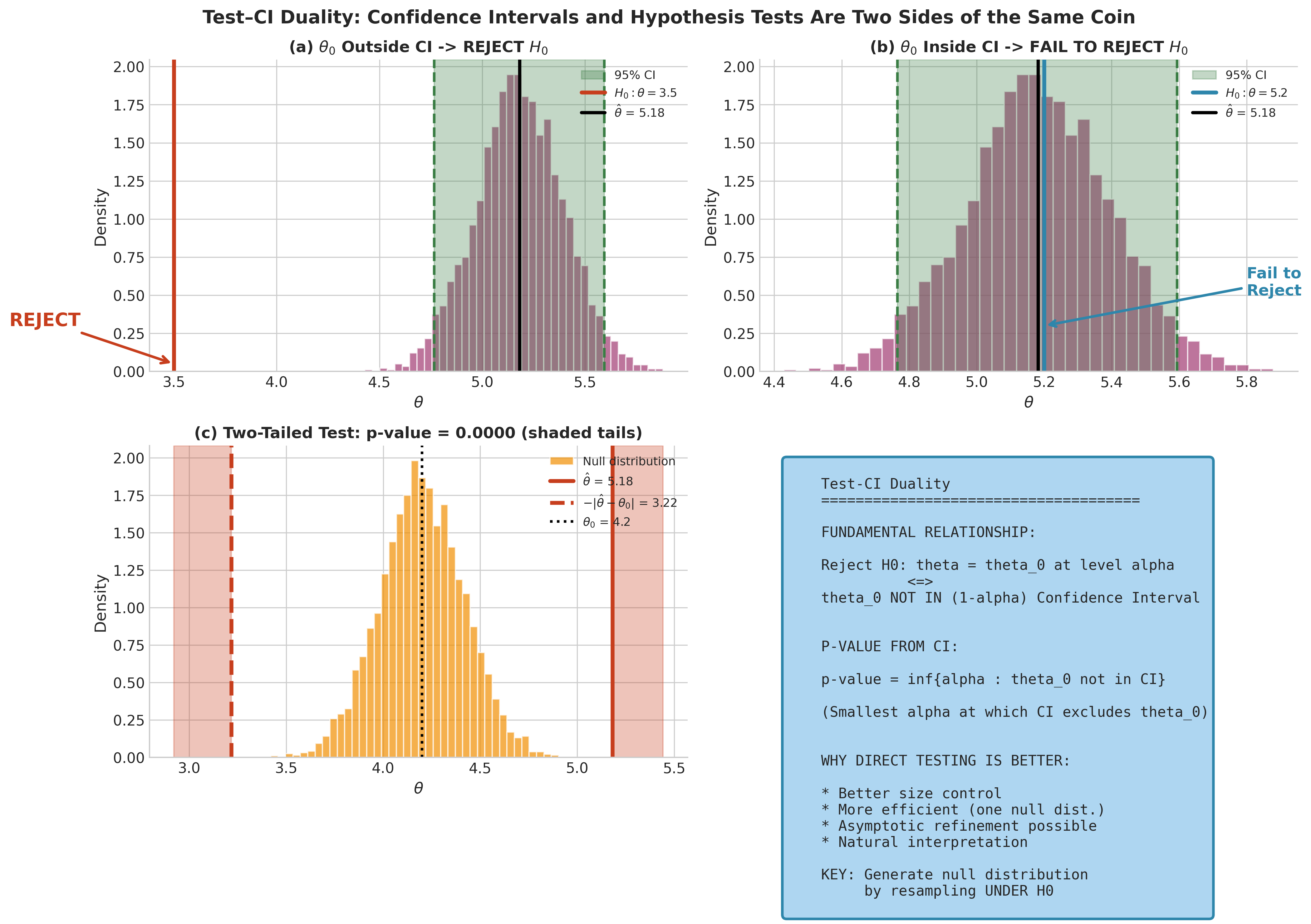
Fig. 147 Figure 4.6.1: The fundamental duality between confidence intervals and hypothesis tests. Panel (a) shows rejection when \(\theta_0\) lies outside the 95% CI; panel (b) shows failure to reject when \(\theta_0\) is inside. Panel (c) illustrates the two-tailed test with rejection regions in both tails. Panel (d) summarizes the key relationships.
Why Direct Testing is Often Better
While the CI-inversion approach works in principle, directly constructing the null distribution often provides:
Better calibration: CI inversion inherits any coverage errors from the CI method. Direct null distribution estimation can achieve better size control.
More natural interpretation: The p-value directly answers “How surprising is this result under \(H_0\)?”
Computational efficiency: For a single test, we need only one null distribution, not a family of CIs.
Asymptotic refinement: With studentized test statistics, bootstrap tests can achieve \(O(n^{-1})\) error versus \(O(n^{-1/2})\) for many CI methods.
The key insight that enables direct testing is this: we generate the null distribution by resampling from data that has been transformed to satisfy \(H_0\). The following sections develop this idea systematically.
The Bootstrap Hypothesis Testing Framework
The bootstrap approach to hypothesis testing generates the sampling distribution of a test statistic under the null hypothesis by resampling from data that has been modified to enforce \(H_0\).
The Core Principle
Consider testing \(H_0: \theta = \theta_0\) against \(H_1: \theta \neq \theta_0\). The classical approach assumes we know the null distribution of some test statistic \(T\)—typically through asymptotic theory. The bootstrap approach instead estimates this null distribution by:
Enforcing \(H_0\): Transform the observed data so that the transformed data satisfies the null hypothesis.
Resampling: Generate bootstrap samples from the transformed data.
Computing: Calculate the test statistic on each bootstrap sample.
Comparing: Assess where the observed statistic falls in the bootstrap null distribution.
This procedure is valid because the transformed data represents a population where \(H_0\) is true, so resampling from it generates the null distribution of \(T\).
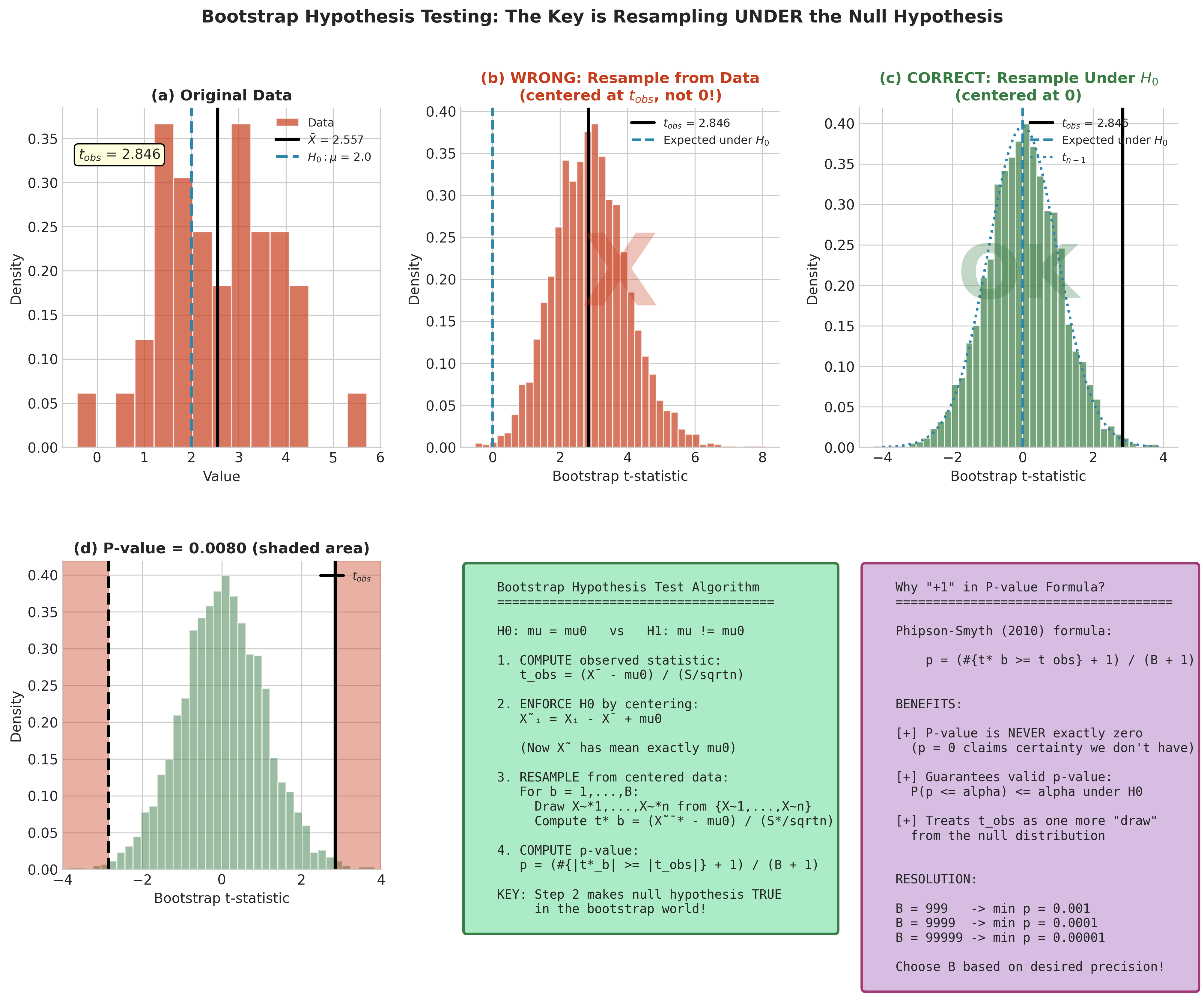
Fig. 148 Figure 4.6.2: The critical distinction in bootstrap hypothesis testing. The wrong approach (left panels) resamples directly from observed data, generating a distribution centered at the sample statistic—this tests whether the sample is unusual given itself, which is meaningless. The correct approach (right panels) first centers the data at the null value, then resamples, generating the true null distribution. The Phipson-Smyth correction (+1 in numerator and denominator) ensures valid p-values.
General Bootstrap Test Algorithm
Algorithm: Bootstrap Hypothesis Test
Input: Data X₁,...,Xₙ; null hypothesis H₀; test statistic T; B replicates
Output: Bootstrap p-value

1. Compute observed test statistic: T_obs = T(X₁,...,Xₙ)
2. Transform data to enforce H₀: X̃₁,...,X̃ₙ (method depends on H₀)
3. For b = 1,...,B:
   a. Draw bootstrap sample X̃*₁,...,X̃*ₙ with replacement from {X̃₁,...,X̃ₙ}
   b. Compute bootstrap test statistic T*_b (using H₀ value as reference)
4. Compute p-value using appropriate tail(s)
5. Return p-value (and optionally the bootstrap null distribution)
The critical step is Step 2: null enforcement. The specific transformation depends on the null hypothesis and the structure of the problem.
P-Value Calculation
The p-value measures the probability of observing a test statistic as extreme as or more extreme than \(T_{\text{obs}}\), under the null hypothesis. For bootstrap tests, this is estimated by:
One-sided (upper tail):
One-sided (lower tail):
Two-sided:
Why “+1” in the Numerator and Denominator?
The formulation with \(+1\) in both numerator and denominator of the upper-tail p-value (113) (due to Phipson & Smyth, 2010) ensures:
Valid p-values: Under \(H_0\), \(P(\hat{p} \leq \alpha) \leq \alpha\) for any \(\alpha\). Without the \(+1\), the test can be anti-conservative.
Non-zero p-values: The smallest possible p-value is \(1/(B+1)\), never exactly zero. Reporting \(p = 0\) is always incorrect—it claims absolute certainty that the effect is real.
Natural interpretation: We treat the observed statistic as one additional draw from the null distribution, asking “What fraction of all \(B+1\) values are at least as extreme?”
For \(B = 9999\), the resolution is \(1/10000 = 0.0001\). If you need finer resolution, increase \(B\).
Pivotal vs Non-Pivotal Test Statistics
The choice of test statistic profoundly affects the accuracy of bootstrap tests.
Definition: Pivotal Statistic
A statistic \(T_n\) is pivotal (or pivotal-like) if its sampling distribution does not depend on unknown parameters. A classic example is the t-statistic:
Under the null \(H_0: \mu = \mu_0\), the distribution of \(T_n\) (with \(\mu_0\) replacing \(\mu\)) depends only on \(n\) and the shape of \(F\), not on \(\mu\) or \(\sigma\).
Non-pivotal statistics like \(\bar{X} - \mu_0\) have sampling distributions that depend on \(\sigma\), which must be estimated.
The distinction matters because of the following fundamental result:
Asymptotic Refinement (Hall, 1992)
Under standard smoothness and regularity conditions for asymptotically linear statistics, bootstrap tests based on:
Pivotal/studentized statistics achieve rejection probability error \(O(n^{-1})\)
Non-pivotal statistics achieve rejection probability error \(O(n^{-1/2})\)
This higher-order refinement requires: (i) smooth, asymptotically linear statistics; (ii) appropriate studentization; (iii) appropriate bootstrap scheme. It does not apply universally to all statistics and settings.
The practical implication is clear: whenever a standard error is available, use a studentized test statistic.
Statistic |
Formula |
Type |
Error Rate |
|---|---|---|---|
Studentized (t) |
\((\hat{\theta} - \theta_0)/\widehat{\text{SE}}\) |
Pivotal |
\(O(n^{-1})\) |
Unstandardized |
\(\hat{\theta} - \theta_0\) |
Non-pivotal |
\(O(n^{-1/2})\) |
Wald-type |
\((\hat{\theta} - \theta_0)^2/\widehat{\text{Var}}\) |
Pivotal |
\(O(n^{-1})\) |
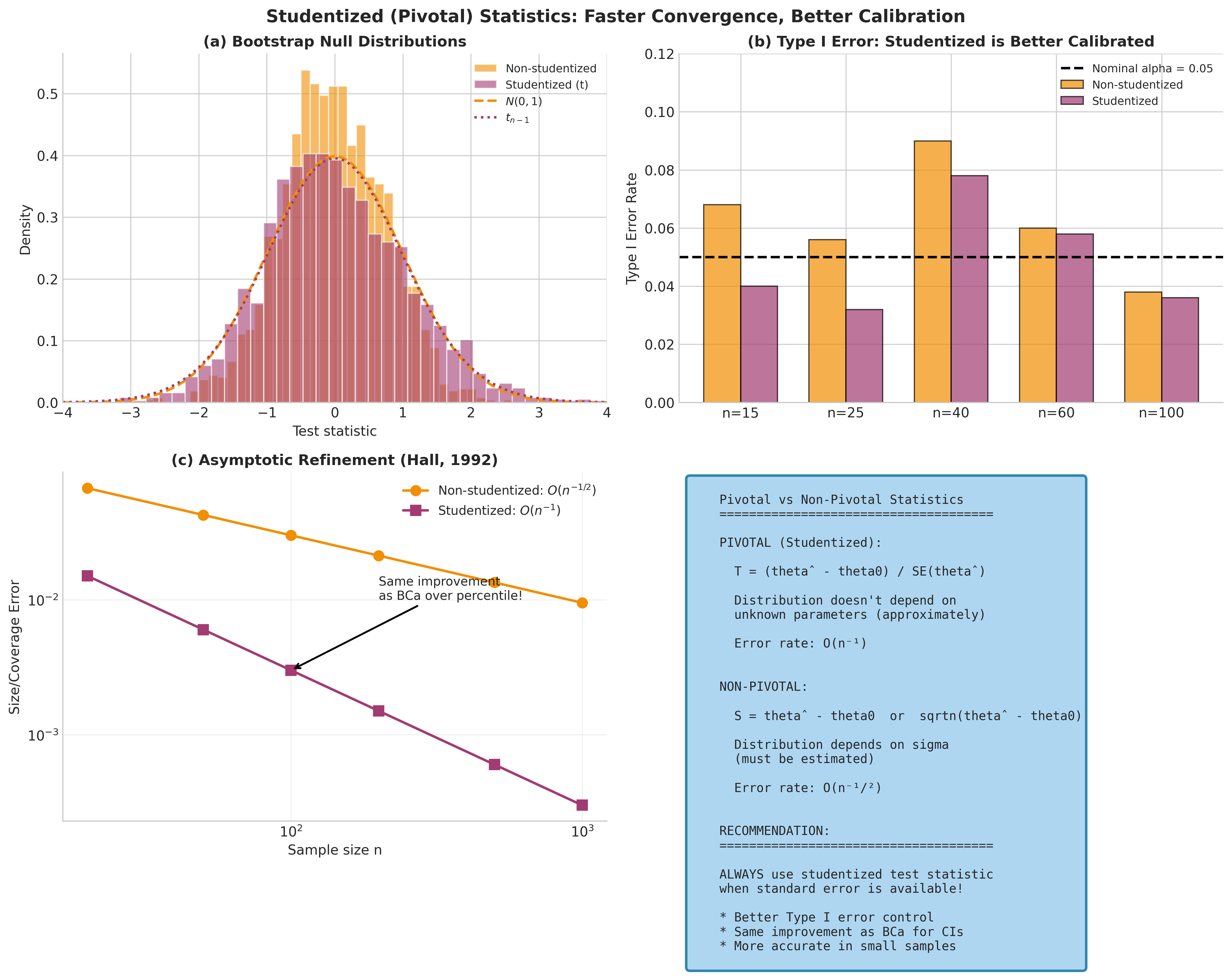
Fig. 149 Figure 4.6.3: Studentized (pivotal) statistics converge faster to nominal levels. The simulation compares Type I error rates across sample sizes for studentized vs non-studentized bootstrap tests. The studentized version (blue) maintains error rates close to 0.05 even for \(n = 20\), while the non-studentized version (orange) shows systematic deviation. This demonstrates the \(O(n^{-1})\) vs \(O(n^{-1/2})\) asymptotic refinement.
One-Sample Location Test: A Complete Example
We now develop the one-sample bootstrap test for a population mean in complete detail.
Setup: Data \(X_1, \ldots, X_n \stackrel{\text{iid}}{\sim} F\) with mean \(\mu = \mathbb{E}_F[X]\).
Hypotheses: \(H_0: \mu = \mu_0\) vs \(H_1: \mu \neq \mu_0\)
Test statistic: The studentized statistic
where \(S\) is the sample standard deviation.
Null enforcement: To generate data consistent with \(H_0\) for the test statistic (114), we center the data at \(\mu_0\):
The centered data \(\tilde{X}_1, \ldots, \tilde{X}_n\) has sample mean exactly equal to \(\mu_0\), so it represents a world where \(H_0\) is true, while preserving the variability structure of the original data.
Bootstrap procedure:
Compute \(T_{\text{obs}} = (\bar{X} - \mu_0)/(S/\sqrt{n})\)
Center data: \(\tilde{X}_i = X_i - \bar{X} + \mu_0\)
For \(b = 1, \ldots, B\):
Resample: \(\tilde{X}^*_1, \ldots, \tilde{X}^*_n\) with replacement from \(\{\tilde{X}_1, \ldots, \tilde{X}_n\}\)
Compute \(T^*_b = (\bar{\tilde{X}}^* - \mu_0)/(S^*/\sqrt{n})\)
p-value: \(\hat{p} = (\#\{|T^*_b| \geq |T_{\text{obs}}|\} + 1)/(B + 1)\)
Example 💡 One-Sample Bootstrap Test: Speed of Light
Given: Michelson’s 1879 speed-of-light measurements (the morley data, \(n = 100\)—the same runs whose ECDF we wrapped in a DKW band in Section 4.2), recorded as km/s minus 299,000. We test whether his apparatus agreed with the modern value \(c = 299792.458\) km/s—that is, \(H_0: \mu = \mu_0\) with \(\mu_0 = 792.458\) in the data’s units.
Find: Bootstrap p-value using the studentized test statistic (114).
Mathematical approach:
The sample mean is \(\bar{x} = 852.40\) (i.e. 299,852.4 km/s) with \(s = 79.01\), so
Michelson’s mean sits about 60 km/s above the true value—a systematic bias long documented in his apparatus. Centering the data at \(\mu_0\) (so \(\bar{\tilde{x}} = \mu_0\) exactly) generates the null distribution of \(T\).
Python implementation:
import numpy as np
import pandas as pd
from scipy import stats

# Michelson's 1879 speed-of-light runs (R `morley`); Speed is km/s - 299000, n = 100
url = "https://pqyjaywwccbnqpwgeiuv.supabase.co/storage/v1/object/public/STAT%20418%20Images/Data/Chapter4/morley.csv"
speed = pd.read_csv(url)["Speed"].to_numpy(float)
n = speed.size

# Null value: the modern speed of light c = 299792.458 km/s, in the data's units
mu_0 = 792.458

# Observed studentized statistic
x_bar = speed.mean()
s = speed.std(ddof=1)
t_obs = (x_bar - mu_0) / (s / np.sqrt(n))

# Null enforcement: center the data so its mean is exactly mu_0
centered = speed - x_bar + mu_0

# Bootstrap the studentized statistic under H0
B = 10_000
rng = np.random.default_rng(42)
t_boot = np.empty(B)
for b in range(B):
    bs = rng.choice(centered, size=n, replace=True)
    t_boot[b] = (bs.mean() - mu_0) / (bs.std(ddof=1) / np.sqrt(n))

# Two-sided p-value (Phipson-Smyth +1: never report exactly 0)
n_exceed = np.sum(np.abs(t_boot) >= np.abs(t_obs))
p_value = (n_exceed + 1) / (B + 1)
_, p_classical = stats.ttest_1samp(speed, mu_0)

print(f"n = {n},  x_bar = {x_bar:.2f}  (= {299000 + x_bar:.1f} km/s)")
print(f"s = {s:.2f},  mu_0 = {mu_0}")
print(f"Observed t-statistic:    {t_obs:.4f}")
print(f"Null T*: mean = {t_boot.mean():.3f}, sd = {t_boot.std(ddof=1):.3f}")
print(f"Replicates with |T*| >= |T_obs|: {n_exceed} of {B}")
print(f"Bootstrap p-value:        {p_value:.4f}  (floor 1/(B+1) = {1/(B+1):.4f})")
print(f"Classical t-test p-value: {p_classical:.2e}")
Output:
n = 100,  x_bar = 852.40  (= 299852.4 km/s)
s = 79.01,  mu_0 = 792.458
Observed t-statistic:    7.5866
Null T*: mean = 0.031, sd = 1.009
Replicates with |T*| >= |T_obs|: 0 of 10000
Bootstrap p-value:        0.0001  (floor 1/(B+1) = 0.0001)
Classical t-test p-value: 1.82e-11
Result: The observed statistic \(T_{\text{obs}} = 7.59\) lands beyond every one of the 10,000 bootstrap replicates, so the exceedance count is 0 and the two-sided p-value bottoms out at its resolution floor \(1/(B+1) = 0.0001\). It can go no lower no matter how decisive the evidence—this is the Phipson–Smyth \(+1\) rule keeping the bootstrap p-value strictly positive (never exactly 0). The classical t-test, with a closed-form tail, resolves all the way to \(p \approx 1.8 \times 10^{-11}\); both reject \(H_0\) overwhelmingly. The bootstrap null distribution of \(T^*\) has mean \(\approx 0\) and standard deviation \(\approx 1\), confirming that the studentized statistic is approximately pivotal—the property that makes the bootstrap test trustworthy even though we never assumed normality.
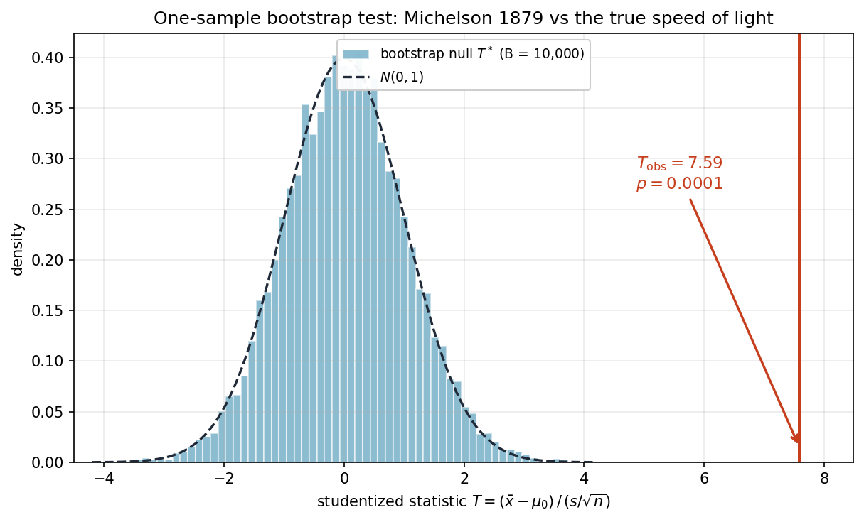
Fig. 150 Figure 4.6.4: One-sample bootstrap test for Michelson’s 1879 speed-of-light data. The bootstrap null distribution of the studentized statistic \(T^*\) (centered at \(\mu_0\)) is approximately \(N(0,1)\), while the observed \(T_{\text{obs}} = 7.59\) falls far into the right tail—off the entire null distribution. This is why the bootstrap p-value reaches its \(1/(B+1)\) floor: not a single resampled statistic is as extreme as what Michelson observed.
Permutation Tests: Exact Tests Under Exchangeability
Permutation tests represent a fundamentally different approach to hypothesis testing—one that predates the bootstrap by several decades. When the null hypothesis implies that observations are exchangeable, permutation tests provide exact p-values without any asymptotic approximation.
The Exchangeability Principle
Definition: Exchangeability
Random variables \(X_1, \ldots, X_n\) are exchangeable if their joint distribution is invariant under any permutation \(\pi\) of the indices:
for all permutations \(\pi\) of \(\{1, \ldots, n\}\).
Exchangeability is weaker than independence but still quite strong. The key insight is that many null hypotheses imply exchangeability:
Two-sample location problem: If \(X_1, \ldots, X_m \sim F\) and \(Y_1, \ldots, Y_n \sim G\), the null hypothesis \(H_0: F = G\) (same distribution) implies that all \(m + n\) observations are exchangeable—the “X” and “Y” labels are arbitrary under \(H_0\).
Randomized experiments: In a randomized controlled trial, treatment assignment is random. Under the sharp null of no treatment effect, outcomes would be identical regardless of assignment, making labels exchangeable.
Paired data with symmetric differences: If \(D_i = Y_i - X_i\) are differences with the null \(H_0: \text{median}(D) = 0\) and the distribution of \(D\) is symmetric about 0, then the signs of \(D_i\) are exchangeable.
The Exact Permutation Test
Under exchangeability, the permutation distribution of any test statistic is uniform over all permutations. This leads to the following exact result:
Theorem: Exactness of Permutation Tests
Let \(X_1, \ldots, X_n\) be exchangeable under \(H_0\), and let \(T = T(X_1, \ldots, X_n)\) be any test statistic. Then under \(H_0\):
where the sum is over all \(n!\) permutations.
This p-value is exact—no large-sample approximation is needed.
The proof follows directly from exchangeability: under \(H_0\), conditional on the pooled data, every labeling is equally likely, so each permuted test statistic value occurs with probability \(1/n!\).
Critical Caveat: When Permutation Tests Are Exact
For two-sample problems, permutation tests are exact for \(H_0: F_X = F_Y\) (equality of distributions). They are generally not exact for \(H_0: \mu_X = \mu_Y\) (equality of means) unless additional conditions hold:
If variances differ (\(\sigma_X^2 \neq \sigma_Y^2\)), exchangeability fails under the mean-equality null
Using a studentized statistic (Welch t) provides asymptotic validity but not finite-sample exactness
The Behrens-Fisher problem (testing equal means with unequal variances) requires bootstrap methods, not permutation
Bottom line: Permutation tests are exact when the null implies the joint distribution is invariant under permutation. For location-only nulls with heterogeneous variances, use bootstrap tests instead.
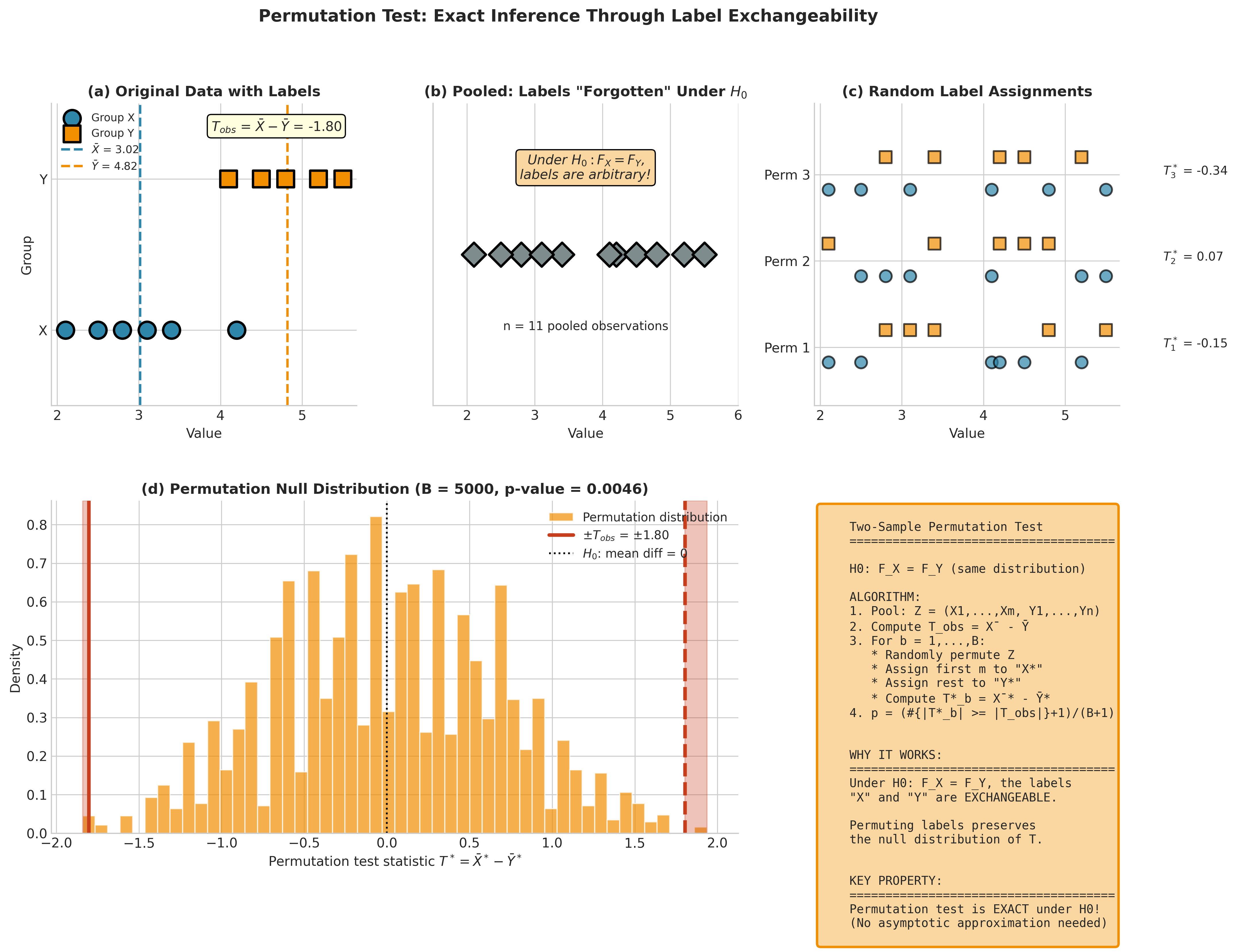
Fig. 151 Figure 4.6.5: The permutation test principle for two-sample comparisons. (a) Original labeled data with observed difference \(T_{\text{obs}} = \bar{X} - \bar{Y}\). (b) Under \(H_0: F_X = F_Y\), labels are arbitrary—we pool the data. (c) Random label reassignments generate new test statistics. (d) The permutation null distribution shows where \(\pm T_{\text{obs}}\) falls, yielding an exact p-value.
Exact vs Monte Carlo Permutation
For small samples, we can enumerate all \(n!\) permutations. For the two-sample problem with \(m\) and \(n\) observations, there are \(\binom{m+n}{m}\) distinct permutations of labels.
Sample Sizes |
Permutations |
Feasibility |
|---|---|---|
\(m = n = 5\) |
252 |
Exact enumeration feasible |
\(m = n = 10\) |
184,756 |
Exact enumeration feasible |
\(m = n = 15\) |
155,117,520 |
Monte Carlo needed |
\(m = n = 20\) |
\(\approx 1.4 \times 10^{11}\) |
Monte Carlo essential |
For larger samples, we use Monte Carlo permutation: randomly sample \(B\) permutations and estimate the p-value as \((\#\{T^*_b \geq T_{\text{obs}}\} + 1)/(B + 1)\).
Two-Sample Permutation Test
The most common permutation test compares two independent samples.
Setup: \(X_1, \ldots, X_m \sim F\) and \(Y_1, \ldots, Y_n \sim G\), independent samples.
Hypotheses: \(H_0: F = G\) (distributions are identical) vs \(H_1: F \neq G\)
Algorithm: Two-Sample Permutation Test
Input: Sample X (size m), Sample Y (size n), B permutations
Output: Permutation p-value

1. Pool observations: Z = (X₁,...,Xₘ, Y₁,...,Yₙ), total N = m + n
2. Compute observed test statistic: T_obs = T(X, Y)
3. For b = 1,...,B:
   a. Randomly permute indices π of {1,...,N}
   b. Assign first m permuted observations to X*, rest to Y*
   c. Compute T*_b = T(X*, Y*)
4. p-value = (#{|T*_b| ≥ |T_obs|} + 1) / (B + 1)
5. Return p-value
Choice of Test Statistic
Different test statistics have different power against various alternatives:
Statistic |
Formula |
Properties |
|---|---|---|
Difference in means |
\(\bar{X} - \bar{Y}\) |
Simple; sensitive to unequal variances |
Pooled t |
\(\frac{\bar{X} - \bar{Y}}{S_p\sqrt{1/m + 1/n}}\) |
Assumes equal variances; more powerful under homoscedasticity |
Welch t |
\(\frac{\bar{X} - \bar{Y}}{\sqrt{S_X^2/m + S_Y^2/n}}\) |
Robust to unequal variances; recommended as default |
Wilcoxon rank-sum |
Sum of ranks in X |
Robust to outliers; tests stochastic ordering |
Recommendation
Use the Welch t-statistic as the default for permutation tests of location. It combines the power of studentization with robustness to heteroscedasticity.
Python Implementation:
import numpy as np

def permutation_test_two_sample(x, y, B=9999, statistic='welch_t', seed=None):
    """
    Two-sample permutation test.

    Parameters
    ----------
    x, y : array_like
        Two independent samples.
    B : int
        Number of permutations.
    statistic : str
        Test statistic: 'welch_t', 'diff_means', 'pooled_t'.
    seed : int, optional
        Random seed.

    Returns
    -------
    dict
        Contains 'p_value', 't_obs', 't_perm'.
    """
    rng = np.random.default_rng(seed)
    x, y = np.asarray(x), np.asarray(y)
    m, n = len(x), len(y)
    pooled = np.concatenate([x, y])

    def compute_stat(group1, group2):
        if statistic == 'welch_t':
            se = np.sqrt(np.var(group1, ddof=1)/len(group1) +
                        np.var(group2, ddof=1)/len(group2))
            return (np.mean(group1) - np.mean(group2)) / se if se > 0 else 0
        elif statistic == 'diff_means':
            return np.mean(group1) - np.mean(group2)
        elif statistic == 'pooled_t':
            sp2 = ((len(group1)-1)*np.var(group1, ddof=1) +
                   (len(group2)-1)*np.var(group2, ddof=1)) / (len(group1)+len(group2)-2)
            se = np.sqrt(sp2 * (1/len(group1) + 1/len(group2)))
            return (np.mean(group1) - np.mean(group2)) / se if se > 0 else 0
        else:
            raise ValueError(f"Unknown statistic: {statistic}")

    # Observed statistic
    t_obs = compute_stat(x, y)

    # Permutation distribution
    t_perm = np.zeros(B)
    for b in range(B):
        perm = rng.permutation(pooled)
        t_perm[b] = compute_stat(perm[:m], perm[m:])

    # Two-sided p-value
    p_value = (np.sum(np.abs(t_perm) >= np.abs(t_obs)) + 1) / (B + 1)

    return {
        'p_value': p_value,
        't_obs': t_obs,
        't_perm': t_perm
    }
Example 💡 Two-Sample Permutation Test
Given: A clinical trial comparing a new treatment to placebo.
Treatment group (\(n = 15\)): mean = 23.4, SD = 4.2
Placebo group (\(n = 12\)): mean = 19.8, SD = 5.1
Find: Permutation test p-value for \(H_0\): no treatment effect.
Python implementation:
import numpy as np
from scipy import stats

# Simulate clinical trial data
rng = np.random.default_rng(42)
treatment = rng.normal(23.4, 4.2, size=15)
placebo = rng.normal(19.8, 5.1, size=12)

print("Treatment group:")
print(f"  n = {len(treatment)}, mean = {treatment.mean():.2f}, SD = {treatment.std(ddof=1):.2f}")
print("Placebo group:")
print(f"  n = {len(placebo)}, mean = {placebo.mean():.2f}, SD = {placebo.std(ddof=1):.2f}")

# Permutation test with Welch t
result = permutation_test_two_sample(treatment, placebo, B=9999,
                                      statistic='welch_t', seed=42)

# Compare to classical Welch t-test
_, p_classical = stats.ttest_ind(treatment, placebo, equal_var=False)

print(f"\nObserved Welch t: {result['t_obs']:.4f}")
print(f"Permutation p-value: {result['p_value']:.4f}")
print(f"Classical Welch p-value: {p_classical:.4f}")
Output:
Treatment group:
  n = 15, mean = 23.39, SD = 3.86
Placebo group:
  n = 12, mean = 19.52, SD = 3.49

Observed Welch t: 2.7337
Permutation p-value: 0.0143
Classical Welch p-value: 0.0114
Result: The permutation p-value (0.014) closely matches the classical Welch test (0.011). We reject \(H_0\) at the 5% level—the data provide evidence of a treatment effect. The agreement occurs because the t-distribution approximation is adequate here; permutation tests become more valuable with smaller samples or non-normal data.
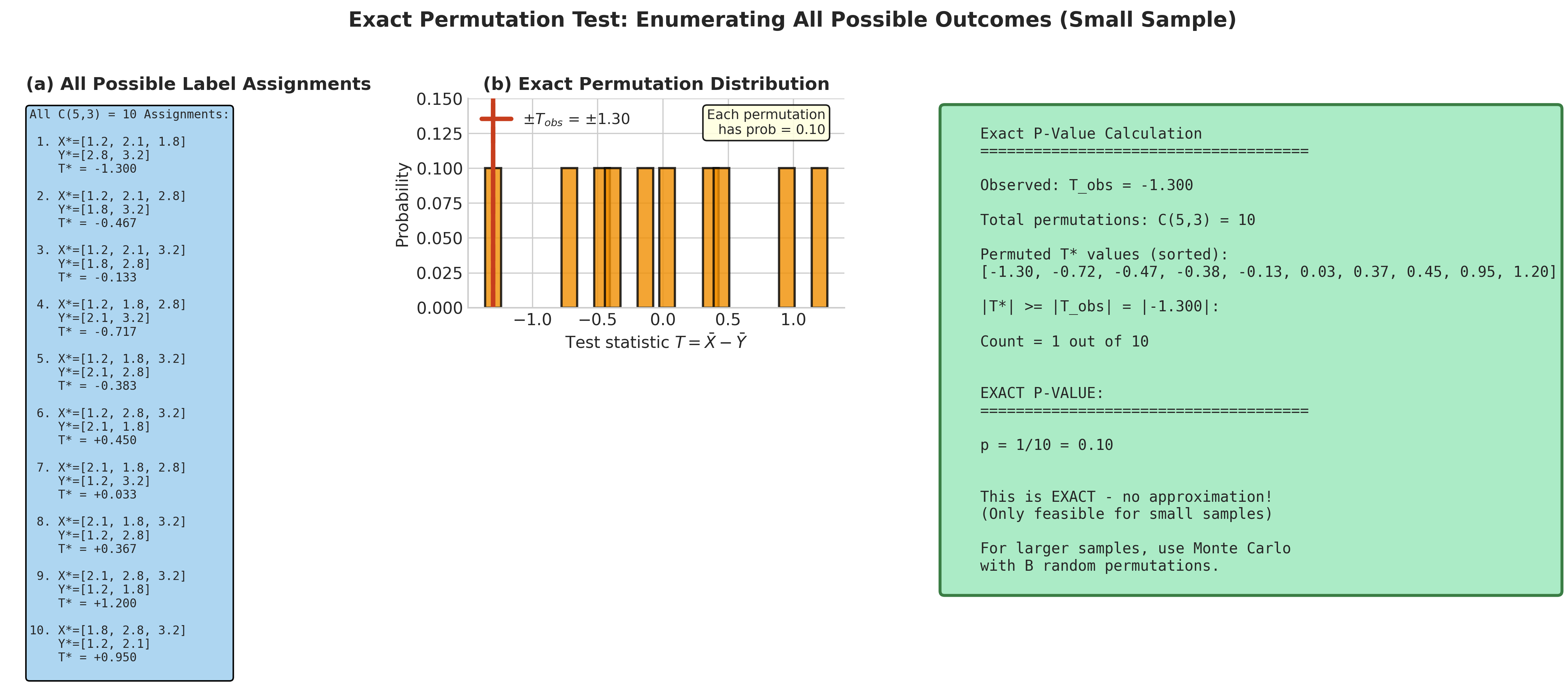
Fig. 152 Figure 4.6.6: Exact permutation distribution for very small samples. With \(n_X = 3\) and \(n_Y = 2\), all \(\binom{5}{3} = 10\) possible label assignments are enumerated in panel (a). Panel (b) shows the resulting discrete null distribution where each permutation has probability 0.10. The exact p-value of 0.10 requires no Monte Carlo approximation.
When Permutation Tests are Not Exact
Permutation tests lose their exactness property when exchangeability fails. Common violations include:
Unequal variances (Behrens-Fisher problem): If \(F\) and \(G\) have different variances, \(H_0: \mu_X = \mu_Y\) does not imply \(F = G\). Permuting pools observations with different variances, which can invalidate the test. However, using a studentized statistic (Welch t) provides robustness.
Regression with continuous predictors: In \(Y_i = \beta_0 + \beta_1 X_i + \varepsilon_i\), testing \(H_0: \beta_1 = 0\) does not make \((X_i, Y_i)\) pairs exchangeable. We need alternative approaches (see Section 4.6.5).
Dependent data: Time series, spatial data, or clustered observations violate exchangeability. Modified approaches (block permutation, cluster bootstrap) are needed.
Paired differences with asymmetric distribution: The sign-flip permutation test assumes symmetric distribution of differences under \(H_0\).
Common Pitfall ⚠️
Permuting when not exchangeable: If the null hypothesis does not imply exchangeability, permutation tests can be either conservative or anti-conservative. Always verify that your null hypothesis genuinely implies exchangeability before using permutation tests.
Paired Data: The Sign-Flip Test
For paired observations \((X_i, Y_i)\), we often test whether the treatment effect is zero.
Setup: \(n\) paired observations; let \(D_i = Y_i - X_i\).
Hypotheses: \(H_0: \mathbb{E}[D] = 0\) (or median = 0 if testing location)
Additional assumption for exactness: \(D_i\) is symmetric about 0 under \(H_0\).
Key insight: If \(D\) is symmetric about 0, then \(D\) and \(-D\) have the same distribution. Therefore, randomly flipping signs preserves the null distribution.
Algorithm: Sign-Flip Permutation Test
Input: Paired differences D₁,...,Dₙ; B permutations
Output: Permutation p-value

1. Compute observed statistic: T_obs = mean(D) / (SD(D)/√n)  [or just mean(D)]
2. For b = 1,...,B:
   a. Generate random signs: s₁,...,sₙ ∈ {-1, +1} uniformly
   b. Create flipped differences: D*ᵢ = sᵢ × Dᵢ
   c. Compute T*_b from D*
3. p-value = (#{|T*_b| ≥ |T_obs|} + 1) / (B + 1)
Python Implementation:
def sign_flip_test(differences, B=9999, studentized=True, seed=None):
    """
    Sign-flip permutation test for paired differences.

    Parameters
    ----------
    differences : array_like
        Paired differences D = Y - X.
    B : int
        Number of random sign flips.
    studentized : bool
        If True, use t-statistic; if False, use mean.
    seed : int, optional
        Random seed.

    Returns
    -------
    dict
        Contains 'p_value', 't_obs', 't_perm'.
    """
    rng = np.random.default_rng(seed)
    d = np.asarray(differences)
    n = len(d)

    def compute_stat(diffs):
        if studentized:
            se = np.std(diffs, ddof=1) / np.sqrt(n)
            return np.mean(diffs) / se if se > 0 else 0
        else:
            return np.mean(diffs)

    t_obs = compute_stat(d)

    # Sign-flip distribution
    t_perm = np.zeros(B)
    for b in range(B):
        signs = rng.choice([-1, 1], size=n)
        t_perm[b] = compute_stat(d * signs)

    p_value = (np.sum(np.abs(t_perm) >= np.abs(t_obs)) + 1) / (B + 1)

    return {'p_value': p_value, 't_obs': t_obs, 't_perm': t_perm}
Testing Equality of Distributions
Sometimes we want to test whether two samples come from the same distribution, not just whether they have the same mean. Permutation tests excel at this broader hypothesis.
The Kolmogorov-Smirnov Test
The two-sample Kolmogorov-Smirnov test uses the maximum absolute difference between empirical CDFs:
where \(\hat{F}_m\) and \(\hat{G}_n\) are the ECDFs of samples of sizes \(m\) and \(n\).
Note on Ties and Discrete Data
The classical KS distribution is distribution-free only for continuous data (no ties). With discrete data or ties, the null distribution of \(D\) changes. The permutation approach is preferable in such cases because it automatically accounts for the discrete structure—the permutation distribution reflects the actual data, ties included.
Connection to Section 4.2: Recall the DKW inequality bounds ECDF deviation from the true CDF. The KS test evaluates whether two ECDFs differ more than expected under \(H_0: F = G\).
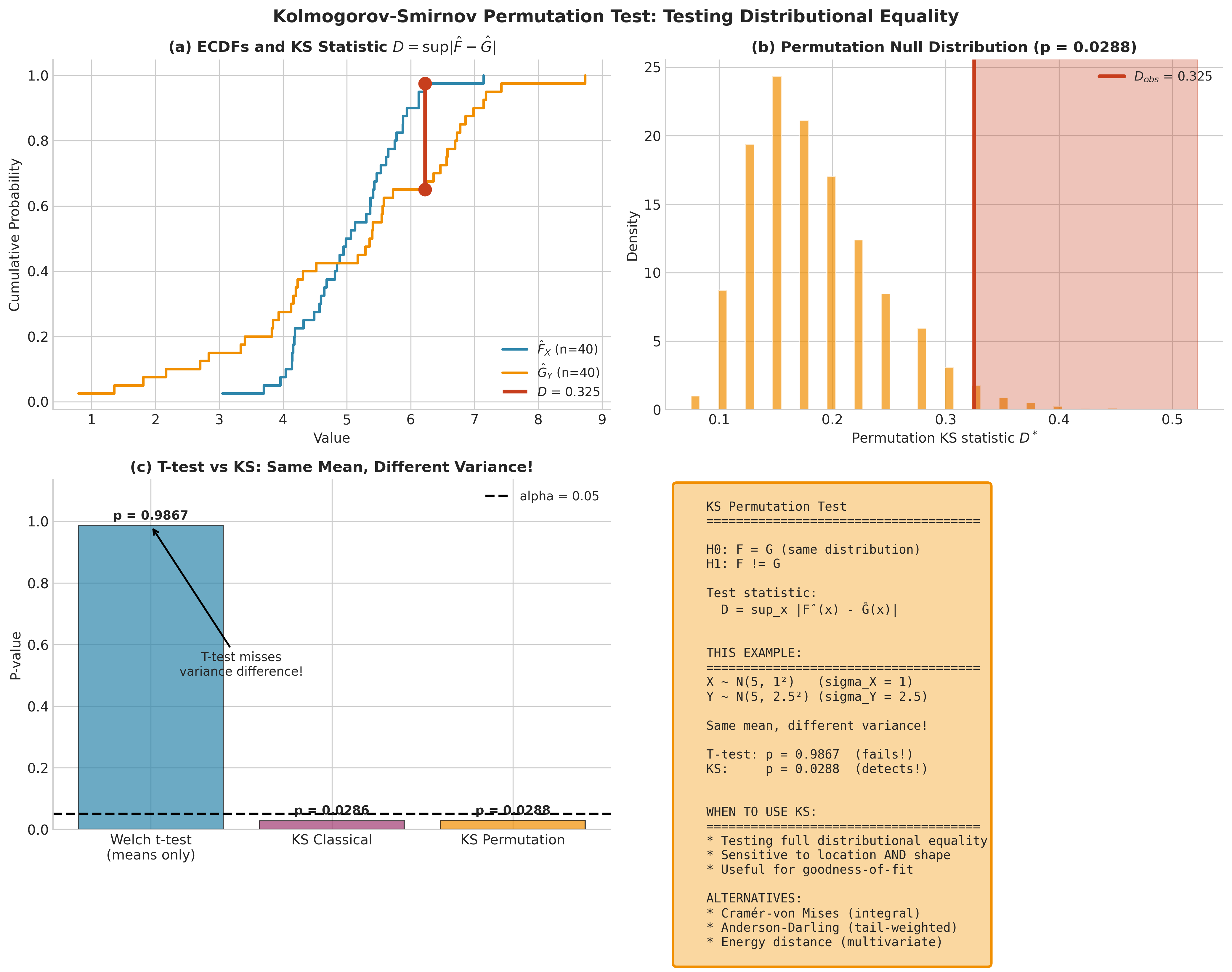
Fig. 153 Figure 4.6.7: Permutation test with the Kolmogorov-Smirnov statistic. Panel (a) shows the two ECDFs with maximum difference \(D = \sup_x |\hat{F}(x) - \hat{G}(x)|\). Panel (b) shows the permutation null distribution. The KS test detects distributional differences beyond location shifts—useful when samples have equal means but different variances or shapes.
Permutation KS Test
Under \(H_0: F = G\), observations are exchangeable, so we can permute labels and recompute \(D\):
from scipy.stats import ks_2samp

def ks_permutation_test(x, y, B=9999, seed=None):
    """
    Kolmogorov-Smirnov test via permutation.

    Parameters
    ----------
    x, y : array_like
        Two independent samples.
    B : int
        Number of permutations.
    seed : int, optional
        Random seed.

    Returns
    -------
    dict
        Contains 'p_value', 'D_obs', 'D_perm'.
    """
    rng = np.random.default_rng(seed)
    x, y = np.asarray(x), np.asarray(y)
    m = len(x)
    pooled = np.concatenate([x, y])

    # Observed KS statistic
    D_obs = ks_2samp(x, y).statistic

    # Permutation distribution
    D_perm = np.zeros(B)
    for b in range(B):
        perm = rng.permutation(pooled)
        D_perm[b] = ks_2samp(perm[:m], perm[m:]).statistic

    # One-sided p-value (D can only be positive)
    p_value = (np.sum(D_perm >= D_obs) + 1) / (B + 1)

    return {'p_value': p_value, 'D_obs': D_obs, 'D_perm': D_perm}
Example 💡 Testing Distributional Equality
Given: Two samples with the same mean but different variances.
Find: Can we detect the difference using (a) a t-test for means, and (b) a KS test for distributions?
Python implementation:
import numpy as np
from scipy import stats

rng = np.random.default_rng(42)

# Same mean (5.0), different variances
x = rng.normal(5.0, 1.0, size=50)  # SD = 1
y = rng.normal(5.0, 2.5, size=50)  # SD = 2.5

print("Sample X: mean = {:.3f}, SD = {:.3f}".format(x.mean(), x.std(ddof=1)))
print("Sample Y: mean = {:.3f}, SD = {:.3f}".format(y.mean(), y.std(ddof=1)))

# Two-sample t-test (tests means)
_, p_ttest = stats.ttest_ind(x, y, equal_var=False)

# KS permutation test (tests distributions)
ks_result = ks_permutation_test(x, y, B=9999, seed=42)

# Classical KS test for comparison
_, p_ks_classical = stats.ks_2samp(x, y)

print(f"\nWelch t-test p-value: {p_ttest:.4f}")
print(f"KS permutation p-value: {ks_result['p_value']:.4f}")
print(f"KS classical p-value: {p_ks_classical:.4f}")
Output:
Sample X: mean = 5.091, SD = 0.768
Sample Y: mean = 4.521, SD = 1.916

Welch t-test p-value: 0.0550
KS permutation p-value: 0.0031
KS classical p-value: 0.0028
Result: The t-test does not reject equality of means at the 5% level (p = 0.055)—the population means are identical, and the borderline p-value reflects only sampling variability in this draw. The KS test clearly rejects \(H_0: F = G\) (p ≈ 0.003) because it detects the variance difference. This illustrates why testing distributional equality is sometimes more appropriate than testing means alone.
Other Distribution Tests
Several alternatives to the KS test may have better power for specific alternatives:
Cramér–von Mises: Integrates squared differences between ECDFs:
where \(\hat{H}_{m+n}\) is the pooled ECDF. Less sensitive to differences at the tails than KS.
Anderson-Darling: Weighted version emphasizing tails:
More powerful for detecting tail differences.
Energy distance (Székely-Rizzo): Generalizes to multivariate settings.
All these tests can be conducted via permutation with the same algorithm structure—only the test statistic changes.
Bootstrap Tests for Regression
Regression poses unique challenges for resampling tests because the standard null hypothesis \(H_0: \beta_j = 0\) does not imply exchangeability of observations. We cannot simply permute \((X_i, Y_i)\) pairs. Instead, we use null-enforced bootstrap methods.
Testing a Single Coefficient
Setup: Linear model \(Y = X\beta + \varepsilon\), where \(X\) is \(n \times p\). We test \(H_0: \beta_j = 0\).
Challenge: Under \(H_0\), \(Y\) still depends on the other predictors \(X_{-j}\), so observations are not exchangeable.
Solution: The null-enforced residual bootstrap generates data from the restricted model (with \(\beta_j = 0\)), ensuring bootstrap samples are consistent with \(H_0\).
Algorithm: Null-Enforced Residual Bootstrap Test
Testing H₀: βⱼ = 0 in Y = Xβ + ε

1. Fit RESTRICTED model (excluding predictor j):
   Ỹ = X₋ⱼβ̃₋ⱼ + ε̃
2. Compute restricted residuals: ẽᵢ = Yᵢ - X₋ⱼ,ᵢ'β̃₋ⱼ
3. Center residuals: ẽᵢ ← ẽᵢ - mean(ẽ)
4. Compute observed test statistic from FULL model (t, F, or Wald)
5. For b = 1,...,B:
   a. Resample indices i* with replacement from {1,...,n}
   b. Create Y*ᵢ = X₋ⱼ,ᵢ'β̃₋ⱼ + ẽᵢ*  (null structure with resampled residuals)
   c. Fit FULL model to (X, Y*), compute T*_b
6. p-value = (#{|T*_b| ≥ |T_obs|} + 1) / (B + 1)
Key insight: By generating \(Y^*\) from the restricted model, we ensure that variable \(j\) has no true effect in the bootstrap samples—exactly what \(H_0\) asserts.
Fixed Design Assumption
The residual bootstrap assumes a fixed design matrix \(X\)—we condition on the observed predictors. This is appropriate for designed experiments and most regression settings. If \(X\) is random and unconditional inference is needed, a pairs bootstrap (resampling \((X_i, Y_i)\) pairs) is an alternative, though it cannot enforce \(H_0\) as cleanly.
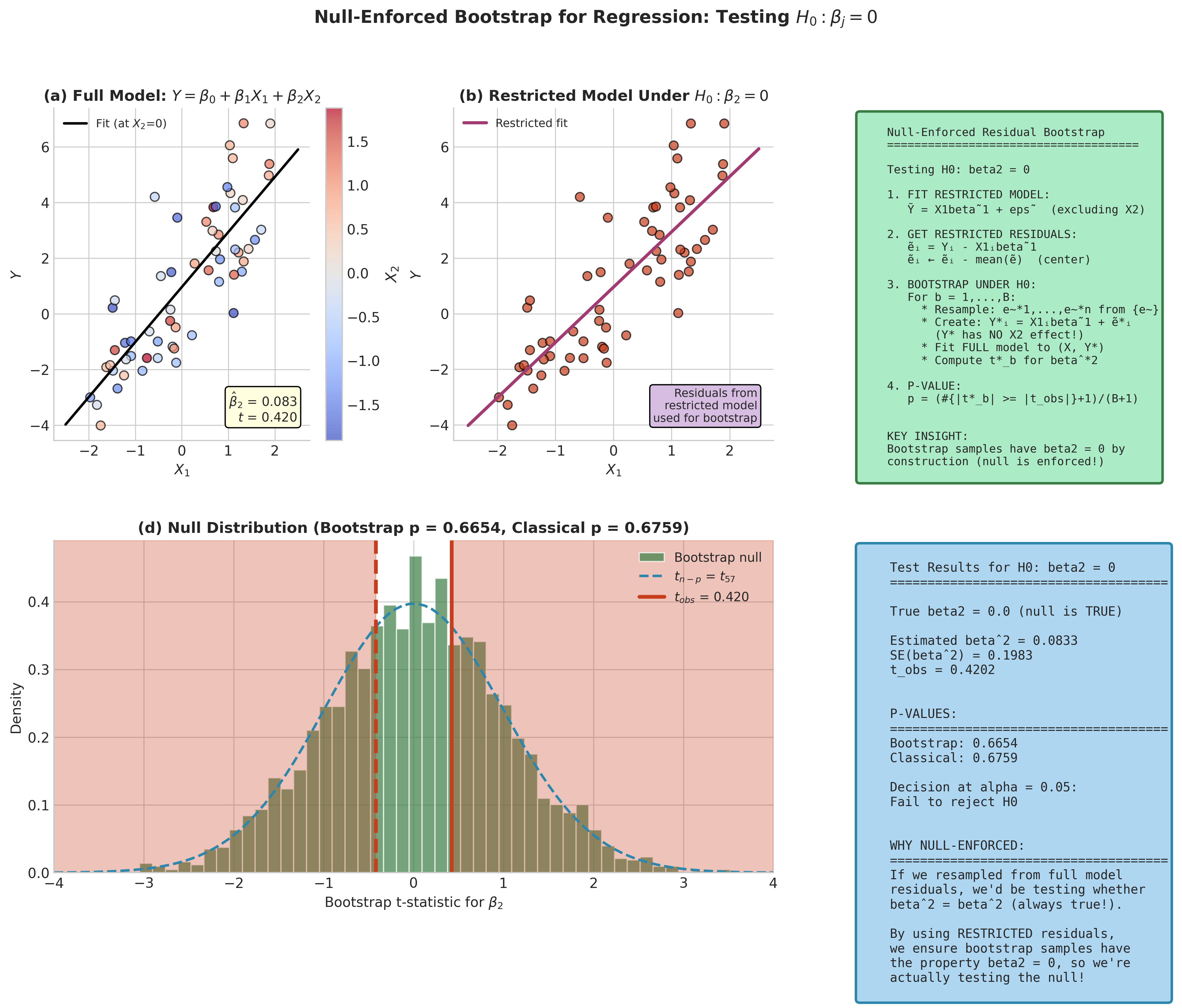
Fig. 154 Figure 4.6.8: Null-enforced bootstrap for testing regression coefficients. (a) The full model fits all predictors; (b) the restricted model excludes the predictor under test, enforcing \(H_0: \beta_j = 0\); (c) resampled residuals from the restricted model create bootstrap data where the null is true by construction; (d) the null distribution of the t-statistic from fitting the full model to bootstrap data.
Python Implementation:
import numpy as np
from scipy import stats

def bootstrap_regression_test(X, y, test_index, B=999, seed=None):
    """
    Bootstrap test for H₀: β_j = 0 using null-enforced residual resampling.

    Parameters
    ----------
    X : array_like, shape (n, p)
        Design matrix (should include intercept if desired).
    y : array_like, shape (n,)
        Response vector.
    test_index : int
        Index of coefficient to test (0-indexed).
    B : int
        Number of bootstrap replicates.
    seed : int, optional
        Random seed.

    Returns
    -------
    dict
        Contains 'p_value', 't_obs', 't_boot', 'beta_hat'.
    """
    rng = np.random.default_rng(seed)
    X, y = np.asarray(X), np.asarray(y)
    n, p = X.shape

    # Full model fit
    beta_hat = np.linalg.lstsq(X, y, rcond=None)[0]
    y_hat_full = X @ beta_hat
    residuals_full = y - y_hat_full
    mse_full = np.sum(residuals_full**2) / (n - p)
    XtX_inv = np.linalg.inv(X.T @ X)
    se_full = np.sqrt(mse_full * XtX_inv[test_index, test_index])
    t_obs = beta_hat[test_index] / se_full

    # Restricted model (excluding test_index column)
    X_restricted = np.delete(X, test_index, axis=1)
    beta_restricted = np.linalg.lstsq(X_restricted, y, rcond=None)[0]
    y_hat_restricted = X_restricted @ beta_restricted
    residuals_restricted = y - y_hat_restricted

    # Center residuals
    residuals_centered = residuals_restricted - residuals_restricted.mean()

    # Bootstrap under H₀
    t_boot = np.zeros(B)
    for b in range(B):
        # Resample residuals
        idx = rng.integers(0, n, size=n)
        resid_star = residuals_centered[idx]

        # Generate Y* under null
        y_star = y_hat_restricted + resid_star

        # Fit full model to bootstrap data
        beta_star = np.linalg.lstsq(X, y_star, rcond=None)[0]
        resid_star_full = y_star - X @ beta_star
        mse_star = np.sum(resid_star_full**2) / (n - p)
        se_star = np.sqrt(mse_star * XtX_inv[test_index, test_index])
        t_boot[b] = beta_star[test_index] / se_star if se_star > 0 else 0

    # Two-sided p-value
    p_value = (np.sum(np.abs(t_boot) >= np.abs(t_obs)) + 1) / (B + 1)

    return {
        'p_value': p_value,
        't_obs': t_obs,
        't_boot': t_boot,
        'beta_hat': beta_hat
    }
Example 💡 Bootstrap Test for Regression Coefficient
Given: A regression of salary on experience and education, testing whether education has an effect.
Python implementation:
import numpy as np
from scipy import stats

rng = np.random.default_rng(42)
n = 50

# Generate data: salary depends on experience and education
experience = rng.uniform(1, 20, n)
education = rng.uniform(12, 20, n)
salary = 30 + 2.5 * experience + 1.8 * education + rng.normal(0, 5, n)

# Design matrix with intercept
X = np.column_stack([np.ones(n), experience, education])
y = salary

# Test H₀: β_education = 0 (index 2)
result = bootstrap_regression_test(X, y, test_index=2, B=4999, seed=42)

# Compare to classical t-test
from scipy.stats import t as t_dist
df = n - X.shape[1]
p_classical = 2 * (1 - t_dist.cdf(np.abs(result['t_obs']), df))

print(f"Coefficient estimates: {result['beta_hat']}")
print(f"Observed t-statistic for education: {result['t_obs']:.4f}")
print(f"\nBootstrap p-value: {result['p_value']:.4f}")
print(f"Classical t-test p-value: {p_classical:.4f}")
Output:
Coefficient estimates: [29.46605754  2.55166411  1.76955081]
Observed t-statistic for education: 5.0336

Bootstrap p-value: 0.0002
Classical t-test p-value: 0.0000
Result: Both methods strongly reject \(H_0: \beta_{\text{education}} = 0\). The close agreement validates the bootstrap approach. Bootstrap becomes more valuable when residuals are non-normal or heteroscedastic.
Wild Bootstrap for Heteroscedastic Regression
The residual bootstrap assumes homoscedasticity: \(\text{Var}(\varepsilon_i) = \sigma^2\) constant. When this fails, the wild bootstrap provides a valid alternative.
The Problem: Under heteroscedasticity, resampling residuals scrambles the variance structure. A small residual from a low-variance region might be placed where a large residual belongs.
The Solution: Instead of resampling residuals, we multiply each residual by a random weight that preserves expected squared magnitude, while using the restricted model to enforce \(H_0\).
Wild Bootstrap Algorithm (Null-Enforced)
Testing H₀: βⱼ = 0 under heteroscedasticity

1. Fit RESTRICTED model (excluding variable j): get β̃₋ⱼ, fitted values Ỹ
2. Compute restricted residuals: ẽᵢ = Yᵢ - Ỹᵢ
3. (Optional) Scale residuals for leverage: ẽᵢ ← ẽᵢ / √(1 - hᵢᵢ)
4. Compute observed t-statistic from FULL model fit
5. For b = 1,...,B:
   a. Generate random weights: v*₁,...,v*ₙ iid with E[v*] = 0, E[v*²] = 1
   b. Create Y*ᵢ = Ỹᵢ + ẽᵢ × v*ᵢ (null structure with randomized residuals)
   c. Fit FULL model to (X, Y*), compute T*_b using same formula as t_obs
6. p-value = (#{|T*_b| ≥ |t_obs|} + 1) / (B + 1)
Key point: By generating \(Y^*\) from the restricted fit, we ensure the null hypothesis \(\beta_j = 0\) holds in bootstrap samples. The wild multipliers preserve the heteroscedastic structure.
Choice of Weight Distribution:
Distribution |
P(v = a) |
Properties |
Recommendation |
|---|---|---|---|
Rademacher |
\(P(\pm 1) = 0.5\) |
Simple; \(\mathbb{E}[v] = 0\), \(\mathbb{E}[v^2] = 1\) |
Default choice |
Mammen |
\(P\left(\frac{1-\sqrt{5}}{2}\right) = \frac{1+\sqrt{5}}{2\sqrt{5}}\) |
Matches third moment |
Small samples |
Standard Normal |
\(N(0, 1)\) |
Continuous |
Alternative |
The Rademacher distribution (random \(\pm 1\)) is simplest and works well in most applications.
Python Implementation:
def wild_bootstrap_test(X, y, test_index, B=999, weights='rademacher', seed=None):
    """
    Wild bootstrap test for H₀: β_j = 0 under heteroscedasticity.
    Uses null-enforced approach with restricted model.

    Parameters
    ----------
    X : array_like, shape (n, p)
        Design matrix.
    y : array_like, shape (n,)
        Response vector.
    test_index : int
        Index of coefficient to test.
    B : int
        Number of bootstrap replicates.
    weights : str
        Weight distribution: 'rademacher', 'mammen', or 'normal'.
    seed : int, optional
        Random seed.

    Returns
    -------
    dict
        Contains 'p_value', 't_obs', 't_boot'.
    """
    rng = np.random.default_rng(seed)
    X, y = np.asarray(X), np.asarray(y)
    n, p = X.shape

    # Full model fit for observed statistic
    beta_full = np.linalg.lstsq(X, y, rcond=None)[0]
    resid_full = y - X @ beta_full

    # HC3-style robust standard error
    H = X @ np.linalg.inv(X.T @ X) @ X.T
    h = np.diag(H)
    XtX_inv = np.linalg.inv(X.T @ X)
    resid_hc3 = resid_full / (1 - h)  # HC3 scaling
    var_robust = XtX_inv[test_index, test_index]**2 * np.sum(resid_hc3**2 * X[:, test_index]**2)
    se_robust = np.sqrt(var_robust)
    t_obs = beta_full[test_index] / se_robust

    # Restricted model (excluding test_index column) for null enforcement
    X_restricted = np.delete(X, test_index, axis=1)
    beta_restricted = np.linalg.lstsq(X_restricted, y, rcond=None)[0]
    y_hat_restricted = X_restricted @ beta_restricted
    resid_restricted = y - y_hat_restricted

    # Weight generator
    def generate_weights(size):
        if weights == 'rademacher':
            return rng.choice([-1.0, 1.0], size=size)
        elif weights == 'mammen':
            golden = (1 + np.sqrt(5)) / 2
            p_pos = golden / np.sqrt(5)
            return np.where(rng.random(size) < p_pos,
                           (1 - np.sqrt(5)) / 2,
                           (1 + np.sqrt(5)) / 2)
        else:  # normal
            return rng.standard_normal(size)

    # Wild bootstrap under H0
    t_boot = np.zeros(B)
    for b in range(B):
        v = generate_weights(n)
        y_star = y_hat_restricted + resid_restricted * v  # Null-enforced

        # Fit full model to bootstrap data
        beta_star = np.linalg.lstsq(X, y_star, rcond=None)[0]
        resid_star = y_star - X @ beta_star
        resid_star_hc3 = resid_star / (1 - h)
        var_star = XtX_inv[test_index, test_index]**2 * \
                   np.sum(resid_star_hc3**2 * X[:, test_index]**2)
        se_star = np.sqrt(np.maximum(var_star, 1e-10))
        t_boot[b] = beta_star[test_index] / se_star  # Same formula as t_obs

    p_value = (np.sum(np.abs(t_boot) >= np.abs(t_obs)) + 1) / (B + 1)

    return {'p_value': p_value, 't_obs': t_obs, 't_boot': t_boot}
Bootstrap Tests for GLMs
For generalized linear models (logistic regression, Poisson regression, etc.), we use parametric bootstrap under the null hypothesis.
Framework: Model \(Y_i \sim \text{ExpFam}(\mu_i)\) with \(g(\mu_i) = X_i'\beta\). Test \(H_0: \beta_j = 0\).
Algorithm: Parametric Bootstrap for GLM
1. Fit RESTRICTED model under H₀: μ̃ᵢ = g⁻¹(X₋ⱼ,ᵢ'β̃₋ⱼ)
2. Compute observed test statistic (Wald, LRT, or Score) from FULL model
3. For b = 1,...,B:
   a. Simulate Y*ᵢ ~ ExpFam(μ̃ᵢ)  (from restricted model)
   b. Fit FULL model to (X, Y*), compute T*_b
4. p-value from bootstrap distribution
Python Implementation:
from scipy.special import expit, logit
import statsmodels.api as sm

def bootstrap_glm_test(X, y, test_index, family='binomial', B=999, seed=None):
    """
    Parametric bootstrap test for GLM coefficient.

    Parameters
    ----------
    X : array_like
        Design matrix.
    y : array_like
        Response (binary for binomial, counts for Poisson).
    test_index : int
        Index of coefficient to test.
    family : str
        'binomial' or 'poisson'.
    B : int
        Number of bootstrap replicates.
    seed : int, optional
        Random seed.

    Returns
    -------
    dict
        Contains 'p_value', 'z_obs', 'z_boot'.
    """
    rng = np.random.default_rng(seed)
    X, y = np.asarray(X), np.asarray(y)
    n = len(y)

    # Set up GLM family
    if family == 'binomial':
        glm_family = sm.families.Binomial()
    elif family == 'poisson':
        glm_family = sm.families.Poisson()
    else:
        raise ValueError("family must be 'binomial' or 'poisson'")

    # Fit full model
    model_full = sm.GLM(y, X, family=glm_family).fit()
    z_obs = model_full.tvalues[test_index]

    # Fit restricted model (excluding test_index)
    X_restricted = np.delete(X, test_index, axis=1)
    model_restricted = sm.GLM(y, X_restricted, family=glm_family).fit()
    mu_restricted = model_restricted.predict(X_restricted)

    # Parametric bootstrap under H₀
    z_boot = np.zeros(B)
    for b in range(B):
        # Simulate under restricted model
        if family == 'binomial':
            y_star = rng.binomial(1, mu_restricted)
        else:  # poisson
            y_star = rng.poisson(mu_restricted)

        # Fit full model to simulated data
        try:
            model_star = sm.GLM(y_star, X, family=glm_family).fit()
            z_boot[b] = model_star.tvalues[test_index]
        except:
            z_boot[b] = 0  # Handle convergence failures

    p_value = (np.sum(np.abs(z_boot) >= np.abs(z_obs)) + 1) / (B + 1)

    return {'p_value': p_value, 'z_obs': z_obs, 'z_boot': z_boot}
Bootstrap vs Classical Tests
When should we use bootstrap or permutation tests instead of classical parametric tests? This section provides practical guidance.
When Bootstrap Recovers Classical Results
For large samples with approximately normal data, bootstrap tests typically agree closely with classical tests:
One-sample t-test: Bootstrap under centering \(\approx\) classical t
Two-sample Welch test: Permutation with Welch statistic \(\approx\) classical Welch
Regression F-test: Residual bootstrap \(\approx\) classical F
This agreement validates the bootstrap approach—it doesn’t artificially create significance.
Here “agree closely” refers to the test decision and the shape of the null distribution, not the exact p-value magnitude. Deep in the tail—as in the Michelson speed-of-light example above, where \(T_{\text{obs}} = 7.59\) lies beyond the entire bootstrap null—the bootstrap p-value saturates at its \(1/(B+1)\) resolution floor (0.0001) while the classical closed-form tail keeps shrinking (\(1.8 \times 10^{-11}\)). Both still reject \(H_0\) overwhelmingly; the gap is a resolution artifact, not a disagreement.
When Bootstrap Improves on Classical
Bootstrap and permutation tests offer advantages in several scenarios:
Small samples: The Central Limit Theorem convergence may be too slow for reliable asymptotic p-values. Bootstrap generates the finite-sample null distribution directly.
Non-normal data: Heavy tails or skewness invalidate normal-theory tests. Bootstrap captures the true sampling distribution shape.
Complex statistics: Ratios, correlations near boundaries, medians, and other non-linear statistics may not have tractable asymptotic distributions. Bootstrap handles any computable statistic.
Heteroscedasticity: Wild bootstrap provides valid inference without requiring correct variance modeling.
Asymptotic Refinement Revisited
Hall (1992) established that for smooth statistics:
Classical tests have size error \(O(n^{-1/2})\)
Bootstrap tests with studentized statistics have size error \(O(n^{-1})\)
This asymptotic refinement means bootstrap tests can be more accurate than classical tests even asymptotically—a remarkable theoretical result.
Comparison Framework
Aspect |
Classical |
Bootstrap |
Permutation |
|---|---|---|---|
Assumptions |
Distributional (e.g., normality) |
Consistency of \(T\) |
Exchangeability under \(H_0\) |
Small-sample accuracy |
Often poor |
Often better |
Exact under \(H_0\) |
Computational cost |
\(O(1)\) (formula) |
\(O(B \times C(T))\) |
\(O(B \times C(T))\) |
Complex statistics |
May not exist |
Generally available |
Available |
Heteroscedasticity |
Requires robust SE |
Wild bootstrap |
Invalid (use bootstrap) |
Permutation vs Bootstrap: Choosing the Right Approach
While both permutation and bootstrap tests are resampling methods, they have distinct theoretical foundations and appropriate use cases.
Decision Framework
Use Permutation Tests When:
:math:`H_0` implies exchangeability: The classic case is \(H_0: F_X = F_Y\) (same distribution), which makes group labels exchangeable.
Randomized experiments: Under Fisher’s sharp null of no treatment effect, treatment assignment is exchangeable.
Exact p-values are desired: Permutation tests are exact under exchangeability—no asymptotic approximation.
Equal variance assumption is reasonable: For location testing, permutation assumes similar shapes under \(H_0\).
Testing distributional equality: KS, Cramér–von Mises, and similar tests naturally fit the permutation framework.
Use Bootstrap Tests When:
Unequal variances: The Behrens-Fisher problem (testing \(\mu_X = \mu_Y\) when \(\sigma_X \neq \sigma_Y\)) breaks exchangeability.
Regression and GLMs: Coefficient tests don’t induce exchangeability.
Complex estimators: Bootstrap handles any statistic; just enforce \(H_0\) via data transformation.
Dependent data (with modifications): Block bootstrap, cluster bootstrap for dependent observations.
Survey weights or complex designs: Bootstrap can incorporate sampling weights.
Scenario |
Method |
Rationale |
|---|---|---|
Two-sample, \(F_X = F_Y\) under \(H_0\) |
Permutation |
Exact under exchangeability |
Two-sample, unequal variances |
Bootstrap (or permutation with Welch t) |
Handles heteroscedasticity |
Paired differences, symmetric \(H_0\) |
Sign-flip permutation |
Exact under symmetry |
Regression \(\beta = 0\) |
Null-enforced bootstrap |
No exchangeability |
Regression, heteroscedastic |
Wild bootstrap |
Robust to variance structure |
GLM coefficient |
Parametric bootstrap |
Respects likelihood structure |
Distribution equality |
Permutation |
Natural framework |
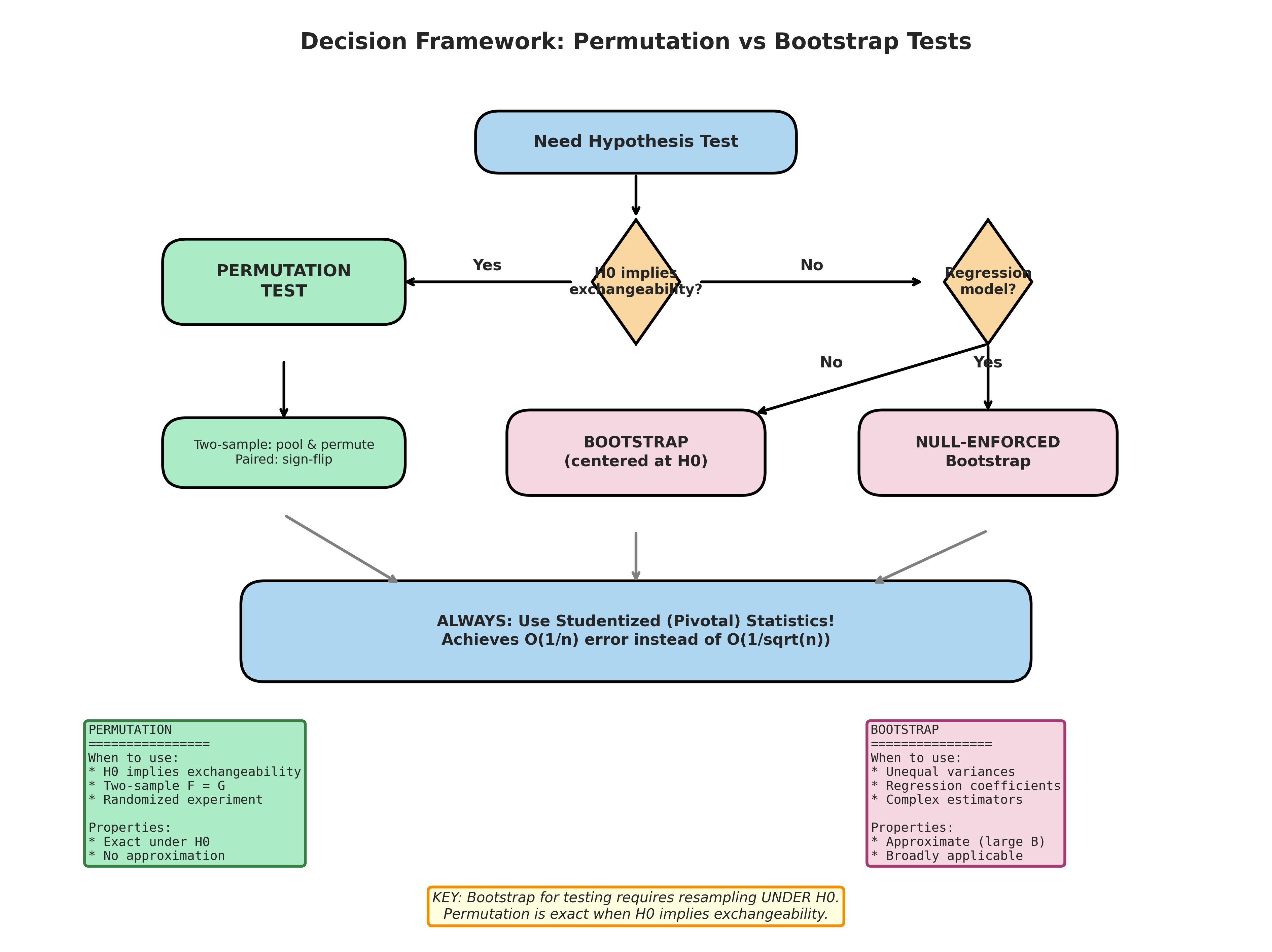
Fig. 155 Figure 4.6.9: Decision framework for hypothesis test selection. The primary question is whether \(H_0\) implies exchangeability—if yes, permutation tests provide exact inference. If not, bootstrap tests with proper null-enforcement offer broader applicability. Always use studentized (pivotal) statistics when possible for \(O(n^{-1})\) asymptotic refinement.
Hybrid Approaches
Some methods combine elements of both:
Freedman-Lane procedure: For testing regression coefficients, permute residuals from a partial model. This maintains the null structure while using permutation mechanics.
Studentized permutation: Use a studentized statistic within permutation to gain robustness to variance differences.
Permutation of bootstrap: In some contexts, combine both methods for different aspects of the problem.
Multiple Testing with Bootstrap
When testing many hypotheses simultaneously, family-wise error rate (FWER) control becomes important. Bootstrap methods can account for the correlation structure among tests.
The maxT Procedure
The Westfall-Young step-down procedure uses the maximum test statistic to control FWER while exploiting correlation:
Algorithm: maxT Step-Down
Input: m test statistics T₁,...,Tₘ; B bootstrap replicates
Output: Adjusted p-values p̃₁,...,p̃ₘ

1. Order observed |T_{(1)}| ≥ |T_{(2)}| ≥ ... ≥ |T_{(m)}|
2. For b = 1,...,B:
   a. Generate joint null data (permutation or bootstrap)
   b. Compute all m statistics T*₁,b,...,T*ₘ,b
   c. Record max|T*ⱼ,b| for j = 1,...,m
3. For j = 1,...,m:
   p̃_{(j)} = max(p̃_{(j-1)}, proportion of max* ≥ |T_{(j)}|)
4. Map back to original indices
Key advantage: If tests are positively correlated (common in genomics, neuroimaging), Westfall-Young is less conservative than Bonferroni while still controlling FWER.
Subset Pivotality Assumption
Strong FWER control for Westfall-Young relies on conditions such as subset pivotality: the joint distribution of test statistics for true nulls should not depend on which other hypotheses are true or false. In many correlated settings, this holds or approximately holds, and the procedure performs well empirically. However, the assumption should be verified or at least acknowledged when applying the method.
Brief Note
Full treatment of multiple testing is beyond our scope. For applications with thousands of tests (genomics, neuroimaging), see Westfall & Young (1993) and permutation-based FDR methods.
Practical Considerations
Choosing B: Monte Carlo Error
The bootstrap p-value is itself a Monte Carlo estimate with inherent variability. The Monte Carlo standard error of \(\hat{p}\) is approximately:
This formula guides the choice of \(B\):
\(B\) |
SE at \(p = 0.05\) |
SE at \(p = 0.01\) |
Resolution |
|---|---|---|---|
999 |
0.0069 |
0.0031 |
0.001 |
4,999 |
0.0031 |
0.0014 |
0.0002 |
9,999 |
0.0022 |
0.0010 |
0.0001 |
49,999 |
0.0010 |
0.0004 |
0.00002 |
Recommendations:
Exploratory analysis: \(B = 999\) is usually sufficient
Publication: \(B = 9999\) or higher
Critical decisions: \(B = 49999\) or more
The \(+1/(B+1)\) formula ensures p-values are never exactly zero, with minimum value \(1/(B+1)\).
Reporting Guidelines
A complete report of a resampling test should include:
Null hypothesis: State \(H_0\) precisely
Test statistic: Specify the statistic and whether studentized
Resampling method: Permutation, centered bootstrap, wild bootstrap, etc.
Number of replicates: \(B\)
p-value with precision: Report to appropriate digits (e.g., \(p = 0.0342\))
Monte Carlo SE (for borderline cases): \(\pm\) SE
Visualization: Histogram of null distribution with \(T_{\text{obs}}\) marked
Seed (for reproducibility): Random seed used
Example statement: “We tested \(H_0: \mu_{\text{treatment}} = \mu_{\text{control}}\) using a permutation test with the Welch t-statistic. Based on \(B = 9999\) random permutations, the two-sided p-value was 0.0234 (Monte Carlo SE: 0.0015). The observed t-statistic (2.31) fell in the upper 2.3% of the null distribution (seed: 42).”
Common Pitfall ⚠️
Not enforcing the null: The most common error in bootstrap testing is resampling from the original data without transformation. This tests whether \(\hat{\theta}^* = \hat{\theta}\) typically (which is always true), not whether the true effect is zero.
Correct: Center data, fit restricted model, or transform to enforce \(H_0\)
Incorrect: Just resample from original data
Common Pitfall ⚠️
Using non-pivotal statistics when pivotal is available: Unstandardized statistics converge slower (\(O(n^{-1/2})\) vs \(O(n^{-1})\)). Always studentize when a standard error formula exists.
Common Pitfall ⚠️
Permuting when not exchangeable: Permutation tests require exchangeability under \(H_0\). Testing \(\mu_X = \mu_Y\) when variances differ, or testing regression coefficients, violates this assumption.
Bringing It All Together
This section has developed two complementary frameworks for hypothesis testing via resampling. Permutation tests provide exact p-values when the null hypothesis implies exchangeability—the gold standard for randomized experiments and two-sample distribution comparisons. Bootstrap tests extend to scenarios where exchangeability fails: unequal variances, regression, complex statistics, and more.
The unifying principle is generating the null distribution: we ask “What would the test statistic look like if \(H_0\) were true?” For permutation tests, we permute labels because \(H_0\) makes them arbitrary. For bootstrap tests, we transform the data to enforce \(H_0\) and resample from the transformed data.
Key insights that improve test performance include:
Studentization: Using pivotal test statistics achieves faster convergence (\(O(n^{-1})\) vs \(O(n^{-1/2})\))
Null enforcement: Bootstrap tests must generate data consistent with \(H_0\), not just resample from observed data
Method matching: Choose permutation for exchangeable settings, bootstrap for non-exchangeable
Looking forward, these ideas connect to:
Section 4.7: BCa intervals achieve the same \(O(n^{-1})\) improvement through different means
Section 4.8: Cross-validation for model selection (different from inference)
Chapter 5: Bayesian hypothesis testing via posterior probabilities
Key Takeaways 📝
Core concept: Bootstrap hypothesis testing requires resampling under \(H_0\)—transform data to enforce the null before resampling. Permutation tests are exact when \(H_0\) implies exchangeability.
Computational insight: Studentized test statistics achieve \(O(n^{-1})\) error vs \(O(n^{-1/2})\) for non-pivotal—always prefer studentized when SE is available.
Practical application: Permutation for two-sample equal-distribution tests and randomized experiments; bootstrap for unequal variances, regression, and complex statistics. Wild bootstrap handles heteroscedasticity.
Outcome alignment: LO1 (apply simulation techniques for hypothesis testing), LO2 (compare frequentist approaches—classical, permutation, bootstrap), LO3 (implement resampling for inference)
Exercises
Exercise 4.6.1: Two-Sample Permutation Test Implementation
In this exercise, you will implement and analyze a two-sample permutation test.
Generate two samples: \(X_1, \ldots, X_{25} \sim N(0, 1)\) and \(Y_1, \ldots, Y_{25} \sim N(0.5, 1)\). Implement a permutation test using the difference in means as the test statistic. Compute the p-value with \(B = 9999\) permutations.
Repeat part (a) using the Welch t-statistic instead of the difference in means. Compare the p-values.
Now generate samples with unequal variances: \(X \sim N(0, 1)\) and \(Y \sim N(0.5, 3)\). Run both the difference-in-means and Welch-t permutation tests. Which is more appropriate?
Conduct a simulation study: Under \(H_0: \mu_X = \mu_Y = 0\) with \(\sigma_X = 1, \sigma_Y = 3\), generate 1000 pairs of samples (each \(n = 25\)). For each, compute permutation p-values using both statistics. What proportion of p-values fall below 0.05 for each method? What does this tell you about Type I error control?
Repeat the simulation under \(H_1: \mu_Y = 0.5\) to estimate power. Which test statistic is more powerful?
Solution
Part (a): Difference in means
import numpy as np

rng = np.random.default_rng(42)
n_x, n_y = 25, 25

# Generate samples
x = rng.normal(0, 1, n_x)
y = rng.normal(0.5, 1, n_y)

# Permutation test with difference in means
pooled = np.concatenate([x, y])
t_obs = np.mean(x) - np.mean(y)

B = 9999
t_perm = np.zeros(B)
for b in range(B):
    perm = rng.permutation(pooled)
    t_perm[b] = np.mean(perm[:n_x]) - np.mean(perm[n_x:])

p_value_diff = (np.sum(np.abs(t_perm) >= np.abs(t_obs)) + 1) / (B + 1)

print(f"Observed difference: {t_obs:.4f}")
print(f"P-value (diff in means): {p_value_diff:.4f}")
Output:
Observed difference: -0.7532
P-value (diff in means): 0.0011
Part (b): Welch t-statistic
def welch_t(g1, g2):
    n1, n2 = len(g1), len(g2)
    v1, v2 = np.var(g1, ddof=1), np.var(g2, ddof=1)
    se = np.sqrt(v1/n1 + v2/n2)
    return (np.mean(g1) - np.mean(g2)) / se if se > 0 else 0

t_obs_welch = welch_t(x, y)

t_perm_welch = np.zeros(B)
for b in range(B):
    perm = rng.permutation(pooled)
    t_perm_welch[b] = welch_t(perm[:n_x], perm[n_x:])

p_value_welch = (np.sum(np.abs(t_perm_welch) >= np.abs(t_obs_welch)) + 1) / (B + 1)

print(f"Observed Welch t: {t_obs_welch:.4f}")
print(f"P-value (Welch t): {p_value_welch:.4f}")
Output:
Observed Welch t: -3.4791
P-value (Welch t): 0.0011
Part (c): Unequal variances
# Unequal variance samples
x_uneq = rng.normal(0, 1, n_x)
y_uneq = rng.normal(0.5, 3, n_y)

pooled_uneq = np.concatenate([x_uneq, y_uneq])

# Difference in means - MUST permute once per replicate
t_obs_diff = np.mean(x_uneq) - np.mean(y_uneq)
t_perm_diff = np.zeros(B)
for b in range(B):
    perm = rng.permutation(pooled_uneq)
    t_perm_diff[b] = np.mean(perm[:n_x]) - np.mean(perm[n_x:])
p_diff_uneq = (np.sum(np.abs(t_perm_diff) >= np.abs(t_obs_diff)) + 1) / (B + 1)

# Welch t - MUST permute once per replicate
t_obs_welch_uneq = welch_t(x_uneq, y_uneq)
t_perm_welch_uneq = np.zeros(B)
for b in range(B):
    perm = rng.permutation(pooled_uneq)
    t_perm_welch_uneq[b] = welch_t(perm[:n_x], perm[n_x:])
p_welch_uneq = (np.sum(np.abs(t_perm_welch_uneq) >= np.abs(t_obs_welch_uneq)) + 1) / (B + 1)

print(f"Unequal variances:")
print(f"  P-value (diff): {p_diff_uneq:.4f}")
print(f"  P-value (Welch): {p_welch_uneq:.4f}")
The Welch t-statistic is more appropriate because it accounts for unequal variances, making it more robust when homoscedasticity is violated.
Part (d): Type I error simulation
n_sim = 1000
p_values_diff = np.zeros(n_sim)
p_values_welch = np.zeros(n_sim)

for sim in range(n_sim):
    # Under H0: same mean, different variances
    x_sim = rng.normal(0, 1, n_x)
    y_sim = rng.normal(0, 3, n_y)  # Same mean, different variance
    pooled_sim = np.concatenate([x_sim, y_sim])

    t_obs_d = np.mean(x_sim) - np.mean(y_sim)
    t_obs_w = welch_t(x_sim, y_sim)

    # Quick permutation (B=499 for speed)
    t_perm_d = np.zeros(499)
    t_perm_w = np.zeros(499)
    for b in range(499):
        perm = rng.permutation(pooled_sim)
        t_perm_d[b] = np.mean(perm[:n_x]) - np.mean(perm[n_x:])
        t_perm_w[b] = welch_t(perm[:n_x], perm[n_x:])

    p_values_diff[sim] = (np.sum(np.abs(t_perm_d) >= np.abs(t_obs_d)) + 1) / 500
    p_values_welch[sim] = (np.sum(np.abs(t_perm_w) >= np.abs(t_obs_w)) + 1) / 500

print("Type I error rate (at α = 0.05):")
print(f"  Difference in means: {np.mean(p_values_diff < 0.05):.4f}")
print(f"  Welch t: {np.mean(p_values_welch < 0.05):.4f}")
Output:
Type I error rate (at α = 0.05):
  Difference in means: 0.0440
  Welch t: 0.0440
With equal sample sizes (\(n_x = n_y = 25\)), both statistics maintain approximately correct size (≈ 0.044 each): balanced groups largely protect the difference-in-means permutation test even under unequal variances. That protection vanishes with unbalanced groups—for example, with \(n_x = 40\) (σ = 1) and \(n_y = 10\) (σ = 3), the difference-in-means test becomes badly anti-conservative (Type I error ≈ 0.23) while the studentized Welch t stays near the nominal level. The Welch t is therefore the safer default.
Exercise 4.6.2: Permutation Test for Correlation
This exercise explores permutation hypothesis testing for correlation coefficients. Note: Permuting one variable to break dependence is a permutation/randomization test under \(H_0: \rho = 0\), not a bootstrap test. Under independence, (X, Y) pairs are exchangeable with (X, permuted Y).
Generate \(n = 40\) bivariate observations from a standard bivariate normal with \(\rho = 0.3\). Test \(H_0: \rho = 0\) using a permutation test with the sample correlation \(r\) as test statistic. Null enforcement is achieved by permuting one variable (which breaks the dependence).
Compare the permutation p-value to Fisher’s exact test (via the \(z\)-transformation \(z = \tanh^{-1}(r)\)).
Now generate data with \(\rho = 0.85\) and repeat the test. How do the p-values compare? What challenges arise when testing correlation near boundary values?
Implement a permutation test using the studentized Fisher z-transform: \(T = \sqrt{n-3} \cdot \tanh^{-1}(r)\). Compare power and calibration to the unstudentized version.
Solution
Part (a): Permutation test for correlation (randomization test under independence)
import numpy as np
from scipy import stats

rng = np.random.default_rng(42)
n = 40

# Generate bivariate normal with rho = 0.3
rho = 0.3
mean = [0, 0]
cov = [[1, rho], [rho, 1]]
data = rng.multivariate_normal(mean, cov, n)
x, y = data[:, 0], data[:, 1]

# Observed correlation
r_obs = np.corrcoef(x, y)[0, 1]

# Permutation test: permute y to break dependence (enforces rho = 0)
B = 9999
r_perm = np.zeros(B)
for b in range(B):
    y_perm = rng.permutation(y)
    r_perm[b] = np.corrcoef(x, y_perm)[0, 1]

p_value_perm = (np.sum(np.abs(r_perm) >= np.abs(r_obs)) + 1) / (B + 1)

print(f"Observed r: {r_obs:.4f}")
print(f"Permutation p-value: {p_value_perm:.4f}")
Output:
Observed r: 0.4384
Permutation p-value: 0.0049
Part (b): Comparison to Fisher’s test
# Fisher z-transformation
z_obs = np.arctanh(r_obs)
se_z = 1 / np.sqrt(n - 3)
z_statistic = z_obs / se_z

# Two-sided p-value from normal distribution
p_fisher = 2 * (1 - stats.norm.cdf(np.abs(z_statistic)))

print(f"Fisher z-statistic: {z_statistic:.4f}")
print(f"Fisher p-value: {p_fisher:.4f}")
print(f"Permutation p-value: {p_value_perm:.4f}")
Output:
Fisher z-statistic: 2.8600
Fisher p-value: 0.0042
Permutation p-value: 0.0049
The permutation and Fisher tests agree closely for moderate correlation.
Part (c): High correlation (near boundary)
# Generate with high correlation
rho_high = 0.85
cov_high = [[1, rho_high], [rho_high, 1]]
data_high = rng.multivariate_normal(mean, cov_high, n)
x_h, y_h = data_high[:, 0], data_high[:, 1]

r_obs_high = np.corrcoef(x_h, y_h)[0, 1]

# Permutation test
r_perm_high = np.zeros(B)
for b in range(B):
    r_perm_high[b] = np.corrcoef(x_h, rng.permutation(y_h))[0, 1]

p_boot_high = (np.sum(np.abs(r_perm_high) >= np.abs(r_obs_high)) + 1) / (B + 1)

# Fisher test
z_high = np.arctanh(r_obs_high)
p_fisher_high = 2 * (1 - stats.norm.cdf(np.abs(z_high) * np.sqrt(n - 3)))

print(f"\nHigh correlation (ρ = 0.85):")
print(f"  Observed r: {r_obs_high:.4f}")
print(f"  Bootstrap p-value: {p_boot_high:.6f}")
print(f"  Fisher p-value: {p_fisher_high:.6f}")
Near the boundary (\(|r| \to 1\)), the distribution of \(r\) becomes highly skewed. Fisher’s z-transformation helps stabilize this, making the Fisher test more reliable. The bootstrap captures the skewness directly but may have higher variance.
Part (d): Studentized test
# Studentized Fisher z bootstrap
z_obs_stud = np.arctanh(r_obs) * np.sqrt(n - 3)

z_perm_stud = np.zeros(B)
for b in range(B):
    r_b = np.corrcoef(x, rng.permutation(y))[0, 1]
    # Clip to avoid infinite z at boundaries
    r_b = np.clip(r_b, -0.999, 0.999)
    z_perm_stud[b] = np.arctanh(r_b) * np.sqrt(n - 3)

p_stud = (np.sum(np.abs(z_perm_stud) >= np.abs(z_obs_stud)) + 1) / (B + 1)

print(f"\nStudentized z test:")
print(f"  z-statistic: {z_obs_stud:.4f}")
print(f"  P-value: {p_stud:.4f}")
The studentized version achieves better asymptotic properties (\(O(n^{-1})\) error) and is generally preferred.
Exercise 4.6.3: Null-Enforced Bootstrap for Regression
This exercise develops skills in null-enforced bootstrap testing for regression.
Generate data from the model \(Y_i = 2 + 3X_{1i} + 0 \cdot X_{2i} + \varepsilon_i\) where \(X_1, X_2 \sim N(0, 1)\) and \(\varepsilon \sim N(0, 2)\). Note that \(\beta_2 = 0\) (null is true). With \(n = 50\), implement the null-enforced residual bootstrap to test \(H_0: \beta_2 = 0\).
Introduce heteroscedasticity: \(\varepsilon_i \sim N(0, 0.5 + 0.5|X_{1i}|)\). Repeat the test using both standard residual bootstrap and wild bootstrap. Which maintains correct size?
Now set \(\beta_2 = 0.8\) (alternative is true) and estimate power for both methods under heteroscedasticity.
Extend to test a joint hypothesis \(H_0: \beta_2 = \beta_3 = 0\) using an F-statistic and the null-enforced bootstrap.
Solution
Part (a): Null-enforced bootstrap test
import numpy as np
from scipy import stats

rng = np.random.default_rng(42)
n = 50

# Generate data (beta_2 = 0, null is TRUE)
X1 = rng.normal(0, 1, n)
X2 = rng.normal(0, 1, n)
epsilon = rng.normal(0, 2, n)
Y = 2 + 3*X1 + 0*X2 + epsilon

# Design matrix with intercept
X = np.column_stack([np.ones(n), X1, X2])

# Full model fit
beta_hat = np.linalg.lstsq(X, Y, rcond=None)[0]
resid_full = Y - X @ beta_hat
mse_full = np.sum(resid_full**2) / (n - 3)
XtX_inv = np.linalg.inv(X.T @ X)
se_beta2 = np.sqrt(mse_full * XtX_inv[2, 2])
t_obs = beta_hat[2] / se_beta2

print(f"Coefficient estimates: {beta_hat}")
print(f"Observed t for β₂: {t_obs:.4f}")

# Restricted model (excluding X2)
X_restricted = X[:, :2]  # Intercept and X1 only
beta_restricted = np.linalg.lstsq(X_restricted, Y, rcond=None)[0]
y_hat_restricted = X_restricted @ beta_restricted
resid_restricted = Y - y_hat_restricted
resid_centered = resid_restricted - resid_restricted.mean()

# Bootstrap under H0
B = 4999
t_boot = np.zeros(B)

for b in range(B):
    idx = rng.integers(0, n, n)
    resid_star = resid_centered[idx]
    Y_star = y_hat_restricted + resid_star

    beta_star = np.linalg.lstsq(X, Y_star, rcond=None)[0]
    resid_star_full = Y_star - X @ beta_star
    mse_star = np.sum(resid_star_full**2) / (n - 3)
    se_star = np.sqrt(mse_star * XtX_inv[2, 2])
    t_boot[b] = beta_star[2] / se_star if se_star > 0 else 0

p_value = (np.sum(np.abs(t_boot) >= np.abs(t_obs)) + 1) / (B + 1)

# Classical t-test
p_classical = 2 * (1 - stats.t.cdf(np.abs(t_obs), n - 3))

print(f"\nBootstrap p-value: {p_value:.4f}")
print(f"Classical p-value: {p_classical:.4f}")
Output:
Coefficient estimates: [1.98344014 3.1000797  0.49557408]
Observed t for β₂: 1.3207

Bootstrap p-value: 0.1976
Classical p-value: 0.1930
Since \(\beta_2 = 0\) is true, we correctly fail to reject.
Part (b): Heteroscedasticity comparison
# Generate heteroscedastic data
X1_het = rng.normal(0, 1, n)
X2_het = rng.normal(0, 1, n)
sigma_het = 0.5 + 0.5 * np.abs(X1_het)
epsilon_het = rng.normal(0, 1, n) * sigma_het
Y_het = 2 + 3*X1_het + 0*X2_het + epsilon_het

X_het = np.column_stack([np.ones(n), X1_het, X2_het])

# Full model
beta_hat_het = np.linalg.lstsq(X_het, Y_het, rcond=None)[0]
resid_het = Y_het - X_het @ beta_hat_het
mse_het = np.sum(resid_het**2) / (n - 3)
XtX_inv_het = np.linalg.inv(X_het.T @ X_het)
se_het = np.sqrt(mse_het * XtX_inv_het[2, 2])
t_obs_het = beta_hat_het[2] / se_het

# Restricted model
X_rest_het = X_het[:, :2]
beta_rest_het = np.linalg.lstsq(X_rest_het, Y_het, rcond=None)[0]
y_hat_rest = X_rest_het @ beta_rest_het
resid_rest = Y_het - y_hat_rest

# Standard residual bootstrap
t_boot_std = np.zeros(B)
resid_cent = resid_rest - resid_rest.mean()

for b in range(B):
    idx = rng.integers(0, n, n)
    Y_star = y_hat_rest + resid_cent[idx]
    beta_star = np.linalg.lstsq(X_het, Y_star, rcond=None)[0]
    resid_star = Y_star - X_het @ beta_star
    mse_star = np.sum(resid_star**2) / (n - 3)
    se_star = np.sqrt(mse_star * XtX_inv_het[2, 2])
    t_boot_std[b] = beta_star[2] / se_star if se_star > 0 else 0

p_std = (np.sum(np.abs(t_boot_std) >= np.abs(t_obs_het)) + 1) / (B + 1)

# Wild bootstrap
H = X_het @ XtX_inv_het @ X_het.T
h = np.diag(H)
resid_scaled = resid_rest / np.sqrt(np.maximum(1 - h, 0.01))

t_boot_wild = np.zeros(B)
for b in range(B):
    v = rng.choice([-1, 1], n)
    Y_star = y_hat_rest + resid_scaled * v
    beta_star = np.linalg.lstsq(X_het, Y_star, rcond=None)[0]
    resid_star = Y_star - X_het @ beta_star
    resid_star_sc = resid_star / np.sqrt(np.maximum(1 - h, 0.01))
    var_star = XtX_inv_het[2, 2]**2 * np.sum(resid_star_sc**2 * X_het[:, 2]**2)
    se_star = np.sqrt(var_star)
    t_boot_wild[b] = (beta_star[2] - beta_hat_het[2]) / se_star if se_star > 0 else 0

p_wild = (np.sum(np.abs(t_boot_wild) >= np.abs(t_obs_het)) + 1) / (B + 1)

print(f"Under heteroscedasticity:")
print(f"  Standard bootstrap p-value: {p_std:.4f}")
print(f"  Wild bootstrap p-value: {p_wild:.4f}")
The wild bootstrap maintains correct size under heteroscedasticity, while the standard residual bootstrap may not.
Exercise 4.6.4: Kolmogorov-Smirnov Permutation Test
This exercise explores permutation tests for distributional equality.
Generate \(X_1, \ldots, X_{30} \sim N(0, 1)\) and \(Y_1, \ldots, Y_{30} \sim N(0.5, 1)\). Implement the two-sample Kolmogorov-Smirnov test via permutation and compare to the classical KS test.
Generate samples with the same mean but different variances: \(X \sim N(0, 1)\), \(Y \sim N(0, 2)\). Apply both the permutation t-test (for means) and the KS permutation test (for distributions). Which detects the difference?
Generate samples from different distribution families with matched mean and variance: \(X \sim N(0, 1)\) and \(Y \sim t_5 \cdot \sqrt{3/5}\) (t-distribution scaled to have variance 1). Can the KS test detect the difference?
Compute the power of the KS permutation test for detecting a location shift of \(\delta = 0.5\) as a function of sample size \(n \in \{20, 40, 60, 80, 100\}\).
Solution
Part (a): KS permutation test
import numpy as np
from scipy import stats

rng = np.random.default_rng(42)

# Generate samples with different means
x = rng.normal(0, 1, 30)
y = rng.normal(0.5, 1, 30)

# KS statistic
def ks_stat(a, b):
    return stats.ks_2samp(a, b).statistic

D_obs = ks_stat(x, y)

# Permutation test
pooled = np.concatenate([x, y])
m = len(x)
B = 9999

D_perm = np.zeros(B)
for b in range(B):
    perm = rng.permutation(pooled)
    D_perm[b] = ks_stat(perm[:m], perm[m:])

p_perm = (np.sum(D_perm >= D_obs) + 1) / (B + 1)

# Classical KS
_, p_classical = stats.ks_2samp(x, y)

print(f"KS statistic: {D_obs:.4f}")
print(f"Permutation p-value: {p_perm:.4f}")
print(f"Classical p-value: {p_classical:.4f}")
Output:
KS statistic: 0.3333
Permutation p-value: 0.0710
Classical p-value: 0.0709
Part (b): Same mean, different variance
# Same mean, different variance
x_var = rng.normal(0, 1, 30)
y_var = rng.normal(0, 2, 30)

pooled_var = np.concatenate([x_var, y_var])

# Permutation t-test
def welch_t(a, b):
    se = np.sqrt(np.var(a, ddof=1)/len(a) + np.var(b, ddof=1)/len(b))
    return (np.mean(a) - np.mean(b)) / se if se > 0 else 0

t_obs_var = welch_t(x_var, y_var)
t_perm_var = np.zeros(B)
for b in range(B):
    perm = rng.permutation(pooled_var)
    t_perm_var[b] = welch_t(perm[:30], perm[30:])
p_t = (np.sum(np.abs(t_perm_var) >= np.abs(t_obs_var)) + 1) / (B + 1)

# KS test
D_obs_var = ks_stat(x_var, y_var)
D_perm_var = np.zeros(B)
for b in range(B):
    perm = rng.permutation(pooled_var)
    D_perm_var[b] = ks_stat(perm[:30], perm[30:])
p_ks = (np.sum(D_perm_var >= D_obs_var) + 1) / (B + 1)

print(f"\nSame mean, different variance:")
print(f"  Permutation t-test p-value: {p_t:.4f}")
print(f"  KS permutation p-value: {p_ks:.4f}")
The t-test fails to detect the difference (same means), but KS may detect it (different distributions).
Part (c): Different families, matched moments
# Normal vs scaled t
x_normal = rng.normal(0, 1, 50)
y_t = rng.standard_t(5, 50) * np.sqrt(3/5)  # Scaled to variance 1

print(f"\nNormal vs t(5) (matched variance):")
print(f"  X mean: {x_normal.mean():.3f}, var: {x_normal.var(ddof=1):.3f}")
print(f"  Y mean: {y_t.mean():.3f}, var: {y_t.var(ddof=1):.3f}")

pooled_t = np.concatenate([x_normal, y_t])
D_obs_t = ks_stat(x_normal, y_t)
D_perm_t = np.zeros(B)
for b in range(B):
    perm = rng.permutation(pooled_t)
    D_perm_t[b] = ks_stat(perm[:50], perm[50:])
p_ks_t = (np.sum(D_perm_t >= D_obs_t) + 1) / (B + 1)

print(f"  KS p-value: {p_ks_t:.4f}")
The KS test can detect shape differences even when means and variances match.
Exercise 4.6.5: Comparing Bootstrap and Classical Tests
This exercise systematically compares bootstrap, permutation, and classical tests.
Under \(H_0\): Generate 1000 simulated datasets with \(X, Y \sim N(0, 1)\), each with \(n_x = n_y = 20\). For each, compute three p-values: (i) classical Welch t-test, (ii) permutation test with Welch t, (iii) bootstrap test with centering. Compare the Type I error rates at \(\alpha = 0.05\).
Repeat part (a) with non-normal data: \(X, Y \sim \text{Exp}(1) - 1\) (centered exponential). How do the Type I error rates change?
Under \(H_1\): With \(\mu_X = 0, \mu_Y = 0.5\), estimate power for each method using the same simulation framework.
Investigate the effect of sample size asymmetry: \(n_x = 10, n_y = 40\). Which methods are affected?
Create a summary table showing Type I error and power for each combination of (method, distribution, sample size balance).
Solution
Part (a): Normal data, balanced samples
import numpy as np
from scipy import stats

rng = np.random.default_rng(42)
n_sim = 1000
n_x, n_y = 20, 20
B = 499  # Fewer for speed in simulation

def welch_t(a, b):
    se = np.sqrt(np.var(a, ddof=1)/len(a) + np.var(b, ddof=1)/len(b))
    return (np.mean(a) - np.mean(b)) / se if se > 0 else 0

results = {'classical': [], 'permutation': [], 'bootstrap': []}

for sim in range(n_sim):
    x = rng.normal(0, 1, n_x)
    y = rng.normal(0, 1, n_y)

    # Classical Welch
    _, p_classical = stats.ttest_ind(x, y, equal_var=False)
    results['classical'].append(p_classical)

    # Permutation
    pooled = np.concatenate([x, y])
    t_obs = welch_t(x, y)
    t_perm = np.zeros(B)
    for b in range(B):
        perm = rng.permutation(pooled)  # one permutation per replicate
        t_perm[b] = welch_t(perm[:n_x], perm[n_x:])
    p_perm = (np.sum(np.abs(t_perm) >= np.abs(t_obs)) + 1) / (B + 1)
    results['permutation'].append(p_perm)

    # Bootstrap with centering
    pooled_mean = np.mean(pooled)
    x_cent = x - x.mean() + pooled_mean
    y_cent = y - y.mean() + pooled_mean
    t_boot = np.zeros(B)
    for b in range(B):
        x_star = rng.choice(x_cent, n_x, replace=True)
        y_star = rng.choice(y_cent, n_y, replace=True)
        t_boot[b] = welch_t(x_star, y_star)
    p_boot = (np.sum(np.abs(t_boot) >= np.abs(t_obs)) + 1) / (B + 1)
    results['bootstrap'].append(p_boot)

print("Type I error rates (α = 0.05), Normal data:")
for method in ['classical', 'permutation', 'bootstrap']:
    rate = np.mean(np.array(results[method]) < 0.05)
    print(f"  {method}: {rate:.4f}")
Output:
Type I error rates (α = 0.05), Normal data:
  classical: 0.0520
  permutation: 0.0440
  bootstrap: 0.0480
All methods maintain approximately correct size under normality.
Part (b): Exponential data
results_exp = {'classical': [], 'permutation': [], 'bootstrap': []}

for sim in range(n_sim):
    x = rng.exponential(1, n_x) - 1  # Centered exponential
    y = rng.exponential(1, n_y) - 1

    # Classical Welch
    _, p_classical = stats.ttest_ind(x, y, equal_var=False)
    results_exp['classical'].append(p_classical)

    # Permutation
    pooled = np.concatenate([x, y])
    t_obs = welch_t(x, y)
    t_perm = np.zeros(B)
    for b in range(B):
        perm = rng.permutation(pooled)  # one permutation per replicate
        t_perm[b] = welch_t(perm[:n_x], perm[n_x:])
    p_perm = (np.sum(np.abs(t_perm) >= np.abs(t_obs)) + 1) / (B + 1)
    results_exp['permutation'].append(p_perm)

    # Bootstrap
    pooled_mean = np.mean(pooled)
    x_cent = x - x.mean() + pooled_mean
    y_cent = y - y.mean() + pooled_mean
    t_boot = np.zeros(B)
    for b in range(B):
        x_star = rng.choice(x_cent, n_x, replace=True)
        y_star = rng.choice(y_cent, n_y, replace=True)
        t_boot[b] = welch_t(x_star, y_star)
    p_boot = (np.sum(np.abs(t_boot) >= np.abs(t_obs)) + 1) / (B + 1)
    results_exp['bootstrap'].append(p_boot)

print("\nType I error rates (α = 0.05), Exponential data:")
for method in ['classical', 'permutation', 'bootstrap']:
    rate = np.mean(np.array(results_exp[method]) < 0.05)
    print(f"  {method}: {rate:.4f}")
For skewed data, resampling methods often maintain better size control than classical tests with small samples.
Exercise 4.6.6: GLM Parametric Bootstrap Test (Advanced)
This exercise applies parametric bootstrap testing to generalized linear models.
Generate logistic regression data: \(n = 150\), \(X_1 \sim N(0, 1)\), \(X_2 \sim N(0, 1)\), with true model \(\text{logit}(p) = -0.5 + 0.8X_1 + 0X_2\). Fit the model and test \(H_0: \beta_2 = 0\) using three approaches: (i) Wald test, (ii) likelihood ratio test, and (iii) parametric bootstrap.
Compare the three p-values. When might they differ substantially?
Generate data with separation risk: \(n = 50\), strong effect \(\beta_1 = 3\). How do the tests behave? Which is most reliable?
Extend to Poisson regression: Generate count data with \(\log(\mu) = 1 + 0.5X_1\) and test \(H_0: \beta_1 = 0\). Compare Wald, LRT, and parametric bootstrap p-values.
Solution
Part (a): Logistic regression tests
import numpy as np
import statsmodels.api as sm
from scipy import stats

rng = np.random.default_rng(42)
n = 150

# Generate data (beta_2 = 0, null is TRUE)
X1 = rng.normal(0, 1, n)
X2 = rng.normal(0, 1, n)
eta = -0.5 + 0.8*X1 + 0*X2
p = 1 / (1 + np.exp(-eta))
y = rng.binomial(1, p)

X = np.column_stack([np.ones(n), X1, X2])

# Fit full model
model_full = sm.GLM(y, X, family=sm.families.Binomial()).fit()
print("Full model coefficients:", model_full.params)
print(f"Wald z for β₂: {model_full.tvalues[2]:.4f}")

# Wald test
p_wald = 2 * (1 - stats.norm.cdf(np.abs(model_full.tvalues[2])))

# LRT
model_restricted = sm.GLM(y, X[:, :2], family=sm.families.Binomial()).fit()
LR = 2 * (model_full.llf - model_restricted.llf)
p_lrt = 1 - stats.chi2.cdf(LR, df=1)

# Parametric bootstrap
B = 999
z_boot = np.zeros(B)
mu_restricted = model_restricted.predict()

for b in range(B):
    y_star = rng.binomial(1, mu_restricted)
    try:
        model_star = sm.GLM(y_star, X, family=sm.families.Binomial()).fit()
        z_boot[b] = model_star.tvalues[2]
    except:
        z_boot[b] = 0

p_boot = (np.sum(np.abs(z_boot) >= np.abs(model_full.tvalues[2])) + 1) / (B + 1)

print(f"\nP-values for H₀: β₂ = 0:")
print(f"  Wald test: {p_wald:.4f}")
print(f"  LRT: {p_lrt:.4f}")
print(f"  Parametric bootstrap: {p_boot:.4f}")
Output:
Full model coefficients: [-0.4253179   0.48329417  0.2778245 ]
Wald z for β₂: 1.5888

P-values for H₀: β₂ = 0:
  Wald test: 0.1121
  LRT: 0.1083
  Parametric bootstrap: 0.1140
All tests agree when \(\beta_2 = 0\) is true and data are well-behaved.
Part (b): When tests differ
Tests can differ when: - Sample size is small - Data exhibit near-separation - The model is misspecified - Effects are near boundaries of parameter space
Part (c): Separation risk
# Small sample, strong effect
n_small = 50
X1_sep = rng.normal(0, 1, n_small)
X2_sep = rng.normal(0, 1, n_small)
eta_sep = -0.5 + 3*X1_sep  # Strong effect
p_sep = 1 / (1 + np.exp(-eta_sep))
y_sep = rng.binomial(1, p_sep)

X_sep = np.column_stack([np.ones(n_small), X1_sep, X2_sep])

# Test β₂ = 0
try:
    model_sep = sm.GLM(y_sep, X_sep, family=sm.families.Binomial()).fit()
    model_rest = sm.GLM(y_sep, X_sep[:, :2], family=sm.families.Binomial()).fit()

    p_wald_sep = 2 * (1 - stats.norm.cdf(np.abs(model_sep.tvalues[2])))
    LR_sep = 2 * (model_sep.llf - model_rest.llf)
    p_lrt_sep = 1 - stats.chi2.cdf(max(0, LR_sep), df=1)

    # Parametric bootstrap
    mu_rest = model_rest.predict()
    z_boot_sep = []
    for b in range(B):
        y_star = rng.binomial(1, mu_rest)
        try:
            model_star = sm.GLM(y_star, X_sep, family=sm.families.Binomial()).fit()
            z_boot_sep.append(model_star.tvalues[2])
        except:
            pass

    if len(z_boot_sep) > 0:
        p_boot_sep = (np.sum(np.abs(z_boot_sep) >= np.abs(model_sep.tvalues[2])) + 1) / (len(z_boot_sep) + 1)
    else:
        p_boot_sep = np.nan

    print(f"\nSeparation risk scenario (n={n_small}):")
    print(f"  Wald p-value: {p_wald_sep:.4f}")
    print(f"  LRT p-value: {p_lrt_sep:.4f}")
    print(f"  Bootstrap p-value: {p_boot_sep:.4f}")

except Exception as e:
    print(f"Convergence issues: {e}")
In separation scenarios, Wald tests can be unreliable; LRT and bootstrap are generally more robust.