Appendix A: Calculus Review
From Formulas to Statistical Reasoning
Calculus in this course is not an end in itself but the engine behind three core statistical workflows. Optimization uses derivatives to find maximum likelihood estimates — setting the score function to zero is just setting a derivative to zero. Uncertainty quantification uses the curvature of the log-likelihood (second derivatives) to measure how precisely the data pinpoint a parameter. Transformation uses change-of-variables formulas (Jacobians) to derive the distributions of functions of random variables. Every major result in Chapters 2–5 rests on one of these three applications.
This appendix develops the calculus tools that the rest of the course assumes. We state results precisely, provide intuition for why each one matters statistically, and verify key results computationally. The proofs that use these tools — the central limit theorem, delta method, Cramér-Rao bound — live in Appendix E. The matrix-specific gradient and Hessian identities used in multivariate estimation live in Appendix B. The iterative optimization and quadrature algorithms live in Appendix C.
Road Map 🧭
Sections 1–2 (Univariate): Differentiation rules — especially logarithmic differentiation and the chain rule — that produce score functions; integration techniques (by parts, change of variables) that compute moments and derive densities
Section 3 (Approximation): Taylor series as the bridge from exact to tractable — first-order gives the delta method, second-order gives the quadratic likelihood approximation and the Wald statistic
Section 4 (Leibniz Rule): Differentiation under the integral sign — the single calculus fact that makes E[score] = 0 and the Fisher information equality work
Sections 5–8 (Multivariate): Gradients, Hessians, the multivariate chain rule, convexity, multivariate Taylor expansions, and Jacobian determinants — the geometry of multi-parameter inference
Prerequisites Check
This appendix assumes familiarity with:
Single-variable calculus: Derivatives, basic integrals, limits
Sigma notation: Sums \(\sum_{i=1}^n\) and their properties
Linear algebra basics: Eigenvalues, definiteness, determinants (Appendix B)
Python/NumPy: Basic array operations (Appendix F: Python Random Generation)
Connection to Course Material
Chapter 2 (Monte Carlo): Change of variables for transformation methods; improper integrals for convergence
Chapter 3 (Parametric Inference): Score functions via chain rule; Taylor expansion of log-likelihood for Newton-Raphson and asymptotic normality; Leibniz rule for Fisher info equivalence; convexity for exponential family MLEs; multivariate chain rule for GLM score vectors
Chapter 4 (Resampling): Delta method as first-order Taylor approximation
Chapter 5 (Bayesian): Laplace approximation for posterior modes; Jacobian for prior/posterior transformations
Univariate Differentiation
Basic Rules
Definition
The derivative of \(f\) at \(x\) is \(f'(x) = \lim_{h \to 0} \frac{f(x+h) - f(x)}{h}\), provided the limit exists. The derivative gives the instantaneous rate of change and the slope of the tangent line at \(x\).
Theorem: Differentiation Rules
For differentiable functions \(f\) and \(g\):
Sum rule: \((f + g)' = f' + g'\)
Product rule: \((fg)' = f'g + fg'\)
Quotient rule: \((f/g)' = (f'g - fg')/g^2\)
Chain rule: \(\frac{d}{dx} f(g(x)) = f'(g(x)) \cdot g'(x)\)
Why the chain rule dominates this course. Nearly every likelihood in parametric statistics involves compositions: the data enter through a sufficient statistic, which enters the log-likelihood through a nonlinear function of the parameter. In generalized linear models (Chapter 3.5), the composition is explicit: the linear predictor \(\boldsymbol{x}^\top \boldsymbol{\beta}\) passes through a link function \(g(\cdot)\) to produce the mean \(\mu\), which enters the log-likelihood. The chain rule is what produces the score vector, the information matrix, and the IRLS weight structure from these compositions.
Logarithmic Differentiation
Definition
For a positive differentiable function \(f(x) > 0\):
Equivalently, \(f'(x) = f(x) \cdot \frac{d}{dx} \log f(x)\).
Why we always work with log-likelihoods. Three reasons make logarithmic differentiation the central tool of likelihood-based inference:
Products become sums. For independent data, \(L(\theta) = \prod_{i=1}^n f(x_i; \theta)\), so \(\ell(\theta) = \log L(\theta) = \sum_{i=1}^n \log f(x_i; \theta)\). Sums are easier to differentiate, and the CLT applies to sums.
Exponential families simplify. If \(f(x; \theta) = h(x) \exp(\eta(\theta) T(x) - A(\eta))\), then \(\log f = \eta T(x) - A(\eta) + \log h(x)\). Differentiating with respect to \(\eta\) is straightforward.
The score has mean zero. The derivative \(U(\theta) = \ell'(\theta)\) satisfies \(\mathbb{E}[U(\theta)] = 0\) at the true parameter — a property that is natural in log space but has no analogue for the raw likelihood. This is proved in the Leibniz Rule section below.
Worked Example: Poisson Score Function. Let \(X_1, \ldots, X_n \overset{\text{iid}}{\sim} \text{Poisson}(\lambda)\). The likelihood is:
Taking the log:
The score function is:
Setting \(U(\hat{\lambda}) = 0\) gives the MLE \(\hat{\lambda} = \bar{X}\).
import numpy as np
from scipy.optimize import approx_fprime

rng = np.random.default_rng(42)

n = 50
lam_true = 3.5
data = rng.poisson(lam_true, n)
sum_x = int(np.sum(data))
xbar = np.mean(data)

def poisson_loglik(lam_arr):
    lam = lam_arr[0]
    if lam <= 0:
        return -1e20
    return float(np.sum(data * np.log(lam) - lam))

def score_analytical(lam):
    return sum_x / lam - n

print(f"Poisson score verification (n={n}, x̄={xbar:.2f})")
print(f"{'λ':>8}  {'Analytical':>12}  {'Numerical':>12}  "
      f"{'Difference':>12}")
print("-" * 50)
for lam in [2.0, 3.0, xbar, 4.0, 5.0]:
    s_anal = score_analytical(lam)
    s_num = approx_fprime(np.array([lam]),
                          poisson_loglik, 1e-8)[0]
    print(f"{lam:>8.2f}  {s_anal:>12.6f}  {s_num:>12.6f}  "
          f"{abs(s_anal - s_num):>12.2e}")

print(f"\nMLE: λ̂ = x̄ = {xbar:.2f}")
print(f"Score at MLE: U({xbar:.2f}) = "
      f"{score_analytical(xbar):.6f}")
Poisson score verification (n=50, x̄=3.42)
       λ    Analytical     Numerical    Difference
--------------------------------------------------
   2.00     35.500000     35.500000      3.11e-07
   3.00      7.000000      6.999998      2.22e-06
   3.42      0.000000     -0.000004      3.55e-06
   4.00     -7.250000     -7.249999      6.00e-07
   5.00    -15.800000    -15.799997      2.86e-06

MLE: λ̂ = x̄ = 3.42
Score at MLE: U(3.42) = 0.000000
The analytical and numerical derivatives agree to within \(\sim 10^{-6}\) at every evaluation point, and the score is exactly zero at the MLE \(\hat{\lambda} = \bar{X}\).
Normal Score for \(\mu\) (brief). For \(X_1, \ldots, X_n \sim N(\mu, \sigma^2)\) with \(\sigma^2\) known, the log-likelihood is \(\ell(\mu) = -\frac{n}{2}\log(2\pi\sigma^2) - \frac{1}{2\sigma^2}\sum(x_i - \mu)^2\). The score is \(U(\mu) = \frac{1}{\sigma^2}\sum(x_i - \mu) = \frac{n}{\sigma^2}(\bar{X} - \mu)\). Setting to zero gives \(\hat{\mu} = \bar{X}\).
Higher Derivatives and the Second Derivative Test
Theorem: Second Derivative Test
At a critical point \(x^*\) where \(f'(x^*) = 0\):
\(f''(x^*) > 0\) implies \(x^*\) is a local minimum
\(f''(x^*) < 0\) implies \(x^*\) is a local maximum
\(f''(x^*) = 0\) is inconclusive
The second derivative as information. At a candidate MLE \(\hat{\theta}\), the quantity \(J(\hat{\theta}) = -\ell''(\hat{\theta})\) is the observed Fisher information. It measures the curvature of the log-likelihood at its peak: a sharply curved peak (large \(J\)) means the data strongly favor \(\hat{\theta}\) over nearby values, implying high precision. A broad, flat peak (small \(J\)) means the data are compatible with a range of parameter values, implying low precision. The standard error of the MLE is approximately \(1/\sqrt{J(\hat{\theta})}\).
Worked Example: Poisson MLE is a Maximum. For the Poisson, \(\ell''(\lambda) = -\sum x_i / \lambda^2\). Since \(\sum x_i > 0\) and \(\lambda > 0\), we have \(\ell''(\lambda) < 0\) for all \(\lambda\) — the log-likelihood is strictly concave, and the MLE is the unique global maximum.
import numpy as np

rng = np.random.default_rng(42)

n = 50
lam_true = 3.5
data = rng.poisson(lam_true, n)
sum_x = int(np.sum(data))
xbar = np.mean(data)

print(f"Poisson log-likelihood analysis "
      f"(n={n}, Σxᵢ={sum_x}, x̄={xbar:.2f})")
print(f"{'λ':>6}  {'ℓ(λ)':>12}  {'ℓ′(λ)':>12}  "
      f"{'ℓ″(λ)':>12}")
print("-" * 48)
for lam in [2.0, 2.5, 3.0, xbar, 3.5, 4.0, 4.5]:
    ll = sum_x * np.log(lam) - n * lam
    score = sum_x / lam - n
    d2 = -sum_x / lam**2
    print(f"{lam:>6.2f}  {ll:>12.4f}  {score:>12.4f}  "
          f"{d2:>12.4f}")

print(f"\nAt MLE λ̂ = {xbar:.2f}:")
print(f"  Score ℓ′({xbar:.2f}) = "
      f"{sum_x/xbar - n:.6f} (zero ✓)")
print(f"  ℓ″({xbar:.2f}) = "
      f"{-sum_x/xbar**2:.4f} < 0 (maximum ✓)")
print(f"  Observed information J({xbar:.2f}) = "
      f"{sum_x/xbar**2:.4f}")
Poisson log-likelihood analysis (n=50, Σxᵢ=171, x̄=3.42)
     λ          ℓ(λ)         ℓ′(λ)         ℓ″(λ)
------------------------------------------------
  2.00       18.5282       35.5000      -42.7500
  2.50       31.6857       18.4000      -27.3600
  3.00       37.8627        7.0000      -19.0000
  3.42       39.2685        0.0000      -14.6199
  3.50       39.2225       -1.1429      -13.9592
  4.00       37.0563       -7.2500      -10.6875
  4.50       32.1972      -12.0000       -8.4444

At MLE λ̂ = 3.42:
  Score ℓ′(3.42) = 0.000000 (zero ✓)
  ℓ″(3.42) = -14.6199 < 0 (maximum ✓)
  Observed information J(3.42) = 14.6199
The log-likelihood peaks at the MLE, the score crosses zero there, and the second derivative is negative everywhere — confirming the global maximum. The observed information \(J(\hat{\lambda}) = 14.62\) gives a standard error of \(1/\sqrt{14.62} \approx 0.26\).
Common Derivatives Reference
The following derivatives appear repeatedly throughout the course:
\(f(x)\) |
\(f'(x)\) |
Where it appears |
|---|---|---|
\(x^n\) |
\(nx^{n-1}\) |
Moment calculations, polynomial likelihoods |
\(e^x\) |
\(e^x\) |
MGFs, exponential family densities |
\(\log x\) |
\(1/x\) |
Log-likelihoods (ubiquitous) |
\((1-p)^x\) |
\((1-p)^x \log(1-p)\) |
Geometric and Negative Binomial likelihoods |
\(\Gamma(\alpha)\) |
\(\Gamma(\alpha)\,\psi(\alpha)\) |
Gamma MLE (digamma function \(\psi\)) |
\(\log \Gamma(\alpha)\) |
\(\psi(\alpha)\) |
Gamma, Beta log-likelihoods |
\(x \log x - x\) |
\(\log x\) |
Stirling’s approximation, entropy |
Integration
Definite Integrals as Expectations
Definition
The expected value of \(g(X)\) where \(X\) has density \(f\) is:
Special cases: \(g(x) = x\) gives the mean; \(g(x) = (x - \mu)^2\) gives the variance; \(g(x) = e^{tx}\) gives the MGF; \(g(x) = \mathbf{1}_{[a,b]}(x)\) gives \(P(a \le X \le b)\).
Intuition. Every integral in this course is either a probability, an expectation, or a normalizing constant. Thinking of integrals as expectations unlocks a powerful verification strategy: if you can sample from \(f\), you can approximate any integral by averaging \(g(X_i)\) over simulated draws. This is the Monte Carlo method developed in Chapter 2.
import numpy as np
from scipy import stats
from scipy.integrate import quad

rng = np.random.default_rng(42)

# Verify E[X²] for Gamma(α=3, β=2) three ways
alpha, beta = 3.0, 2.0

# Analytical: E[X²] = Var(X) + (E[X])² = α/β² + (α/β)²
analytical = alpha / beta**2 + (alpha / beta)**2

# scipy.integrate.quad
integrand = lambda x: x**2 * stats.gamma.pdf(
    x, a=alpha, scale=1/beta)
quad_result, _ = quad(integrand, 0, np.inf)

# Monte Carlo
samples = rng.gamma(alpha, 1/beta, 100000)
mc_result = np.mean(samples**2)

print("Verification: E[X²] for Gamma(α=3, β=2)")
print(f"{'Method':>20}  {'E[X²]':>10}  "
      f"{'Error':>12}")
print("-" * 48)
print(f"{'Analytical':>20}  {analytical:>10.6f}  "
      f"{'—':>12}")
print(f"{'scipy.integrate':>20}  {quad_result:>10.6f}  "
      f"{abs(quad_result - analytical):>12.2e}")
print(f"{'Monte Carlo (n=10⁵)':>20}  {mc_result:>10.6f}  "
      f"{abs(mc_result - analytical):>12.2e}")
Verification: E[X²] for Gamma(α=3, β=2)
              Method       E[X²]         Error
------------------------------------------------
          Analytical    3.000000             —
     scipy.integrate    3.000000      0.00e+00
 Monte Carlo (n=10⁵)    3.010147      1.01e-02
All three methods agree. The Monte Carlo estimate is within 0.3% of the exact value — typical for \(10^5\) samples.
Integration by Parts
Theorem: Integration by Parts
Equivalently, \(\int_a^b u(x) v'(x)\,dx = [u(x)v(x)]_a^b - \int_a^b u'(x) v(x)\,dx\).
Intuition. Integration by parts trades one integral for another. The art is choosing \(u\) and \(dv\) so that the new integral \(\int v\,du\) is simpler than the original. In statistics, the typical pattern is: \(u = x^k\) (a power that decreases when differentiated) and \(dv = e^{-\beta x} dx\) (an exponential that stays exponential when integrated).
Worked Example: \(\mathbb{E}[X]\) for Gamma \((\alpha, \beta)\) via IBP.
Set \(u = x^\alpha\) and \(dv = e^{-\beta x}\,dx\), giving \(du = \alpha x^{\alpha-1}\,dx\) and \(v = -e^{-\beta x}/\beta\). The boundary term \([uv]_0^\infty = 0\), since \(x^\alpha(-e^{-\beta x}/\beta) \to 0\) at both limits: the exponential dominates as \(x \to \infty\), and \(x^\alpha \to 0\) at \(x = 0\) because \(\alpha > 0\). Then:
Substituting back: \(\mathbb{E}[X] = \frac{\beta^\alpha}{\Gamma(\alpha)} \cdot \frac{\alpha}{\beta} \cdot \frac{\Gamma(\alpha)}{\beta^\alpha} = \frac{\alpha}{\beta}\).
import numpy as np

rng = np.random.default_rng(42)

alpha, beta = 3.0, 2.0
n_samples = 100000
samples = rng.gamma(alpha, 1/beta, n_samples)

print(f"Verification: E[X] for Gamma(α={alpha}, β={beta})")
print(f"Theoretical E[X] = α/β = {alpha/beta:.6f}")
print(f"Simulated mean    = {np.mean(samples):.6f}")
print(f"Difference        = "
      f"{abs(np.mean(samples) - alpha/beta):.6f}")
Verification: E[X] for Gamma(α=3.0, β=2.0)
Theoretical E[X] = α/β = 1.500000
Simulated mean    = 1.500859
Difference        = 0.000859
Brief second example: For \(X \sim \text{Exp}(\lambda)\), \(\mathbb{E}[X] = \int_0^\infty x \lambda e^{-\lambda x}\,dx\). Setting \(u = x\), \(dv = \lambda e^{-\lambda x}\,dx\) gives \([uv]_0^\infty = 0\) and \(\int_0^\infty e^{-\lambda x}\,dx = 1/\lambda\), so \(\mathbb{E}[X] = 1/\lambda\). This is the \(\alpha = 1\) special case of the Gamma result above.
Change of Variables — Univariate
Theorem: Univariate Change of Variables
If \(Y = g(X)\) where \(g\) is monotone and differentiable with inverse \(g^{-1}\), then:
Intuition. Densities are not probabilities — they measure probability per unit length. When a transformation stretches the \(x\)-axis, the same total probability is spread over a wider interval, so the density must decrease. The factor \(|dx/dy|\) is the “stretching factor” that adjusts the density to preserve total probability. This is the univariate Jacobian.
Worked Example: Inverse CDF Method for the Exponential. Let \(U \sim \text{Uniform}(0, 1)\) and define \(X = -\log(U)/\lambda\). Then \(g^{-1}(x) = e^{-\lambda x}\) and \(|dg^{-1}/dx| = \lambda e^{-\lambda x}\), so:
for \(x > 0\), which is the \(\text{Exp}(\lambda)\) density. This is the inverse CDF method — the foundation of simulation-based inference in Chapter 2.
The multivariate analogue of this result uses the Jacobian determinant; see the Multiple Integrals section below.
Improper Integrals and Convergence
An improper integral \(\int_0^\infty f(x)\,dx\) converges if \(\lim_{M \to \infty} \int_0^M f(x)\,dx\) exists and is finite.
Comparison test: If \(0 \le f(x) \le g(x)\) for all \(x \ge a\) and \(\int_a^\infty g(x)\,dx\) converges, then \(\int_a^\infty f(x)\,dx\) converges.
Statistical relevance. Normalizing constants require convergent integrals: \(\int f(x; \theta)\,dx = 1\). Not all moments exist — the Cauchy distribution has no mean because \(\int |x|/(1+x^2)\,dx\) diverges. Monte Carlo estimation of \(\mathbb{E}[g(X)]\) requires finite \(\text{Var}(g(X))\); when this fails, variance reduction techniques (Chapter 2.5) are needed.
Taylor Series and Approximation
Taylor’s Theorem
Theorem: Taylor’s Theorem with Lagrange Remainder
If \(f\) has \((n+1)\) continuous derivatives on an interval containing \(a\) and \(x\), then:
where the remainder satisfies \(R_n(x) = \frac{f^{(n+1)}(c)}{(n+1)!}(x-a)^{n+1}\) for some \(c\) between \(a\) and \(x\).
Intuition. Taylor’s theorem says any sufficiently smooth function is locally polynomial. The first-order Taylor polynomial is the tangent line; the second-order is the best-fit parabola; each additional term captures higher-order curvature. The remainder \(R_n\) quantifies the approximation error, and its \((x-a)^{n+1}\) factor shows that accuracy improves rapidly close to the expansion point. For log-likelihoods near the MLE, the second-order Taylor approximation is a quadratic — and a quadratic in the exponent of \(L(\theta) = e^{\ell(\theta)}\) produces a normal distribution.
Definition
Big-O and little-o notation. We write \(f(x) = O(g(x))\) as \(x \to a\) if \(|f(x)| \le C|g(x)|\) for some constant \(C\) and all \(x\) near \(a\). We write \(f(x) = o(g(x))\) if \(f(x)/g(x) \to 0\) as \(x \to a\). In Taylor expansions, \(R_n(x) = O((x-a)^{n+1})\) means the error shrinks at least as fast as the \((n+1)\)-th power of the distance from \(a\).
import numpy as np

def taylor_log1px(x, order):
    """Taylor polynomial of log(1+x) about x=0."""
    result = 0.0
    for k in range(1, order + 1):
        result += ((-1) ** (k + 1)) * x ** k / k
    return result

print("Taylor approximations of log(1+x) at selected points")
print(f"{'x':>6}  {'Exact':>10}  {'T₁':>10}  {'T₂':>10}  "
      f"{'T₃':>10}  {'T₄':>10}")
print("-" * 62)
for x in [0.1, 0.3, 0.5, 0.8, 1.0, 1.5]:
    exact = np.log(1 + x)
    vals = [taylor_log1px(x, k) for k in [1, 2, 3, 4]]
    print(f"{x:>6.1f}  {exact:>10.6f}  {vals[0]:>10.6f}  "
          f"{vals[1]:>10.6f}  {vals[2]:>10.6f}  "
          f"{vals[3]:>10.6f}")

print("\nAbsolute errors |log(1+x) - Tₙ(x)|:")
print(f"{'x':>6}  {'|E₁|':>10}  {'|E₂|':>10}  "
      f"{'|E₃|':>10}  {'|E₄|':>10}")
print("-" * 46)
for x in [0.1, 0.3, 0.5, 0.8, 1.0, 1.5]:
    exact = np.log(1 + x)
    errs = [abs(exact - taylor_log1px(x, k))
            for k in [1, 2, 3, 4]]
    print(f"{x:>6.1f}  {errs[0]:>10.2e}  {errs[1]:>10.2e}  "
          f"{errs[2]:>10.2e}  {errs[3]:>10.2e}")
Taylor approximations of log(1+x) at selected points
     x       Exact          T₁          T₂          T₃          T₄
--------------------------------------------------------------
   0.1    0.095310    0.100000    0.095000    0.095333    0.095308
   0.3    0.262364    0.300000    0.255000    0.264000    0.261975
   0.5    0.405465    0.500000    0.375000    0.416667    0.401042
   0.8    0.587787    0.800000    0.480000    0.650667    0.548267
   1.0    0.693147    1.000000    0.500000    0.833333    0.583333
   1.5    0.916291    1.500000    0.375000    1.500000    0.234375

Absolute errors |log(1+x) - Tₙ(x)|:
     x        |E₁|        |E₂|        |E₃|        |E₄|
----------------------------------------------
   0.1    4.69e-03    3.10e-04    2.32e-05    1.85e-06
   0.3    3.76e-02    7.36e-03    1.64e-03    3.89e-04
   0.5    9.45e-02    3.05e-02    1.12e-02    4.42e-03
   0.8    2.12e-01    1.08e-01    6.29e-02    3.95e-02
   1.0    3.07e-01    1.93e-01    1.40e-01    1.10e-01
   1.5    5.84e-01    5.41e-01    5.84e-01    6.82e-01
Near \(x = 0\) (where the expansion is centered), the errors decrease dramatically with each additional term — the 4th-order error at \(x = 0.1\) is \(\sim 10^{-6}\). At \(x = 1.5\), even the 4th-order polynomial is inaccurate — this is near the boundary of convergence (the Taylor series for \(\log(1+x)\) converges exactly for \(-1 < x \le 1\)). Figure A.1 plots these polynomial approximations and the growth of their errors away from the expansion point.
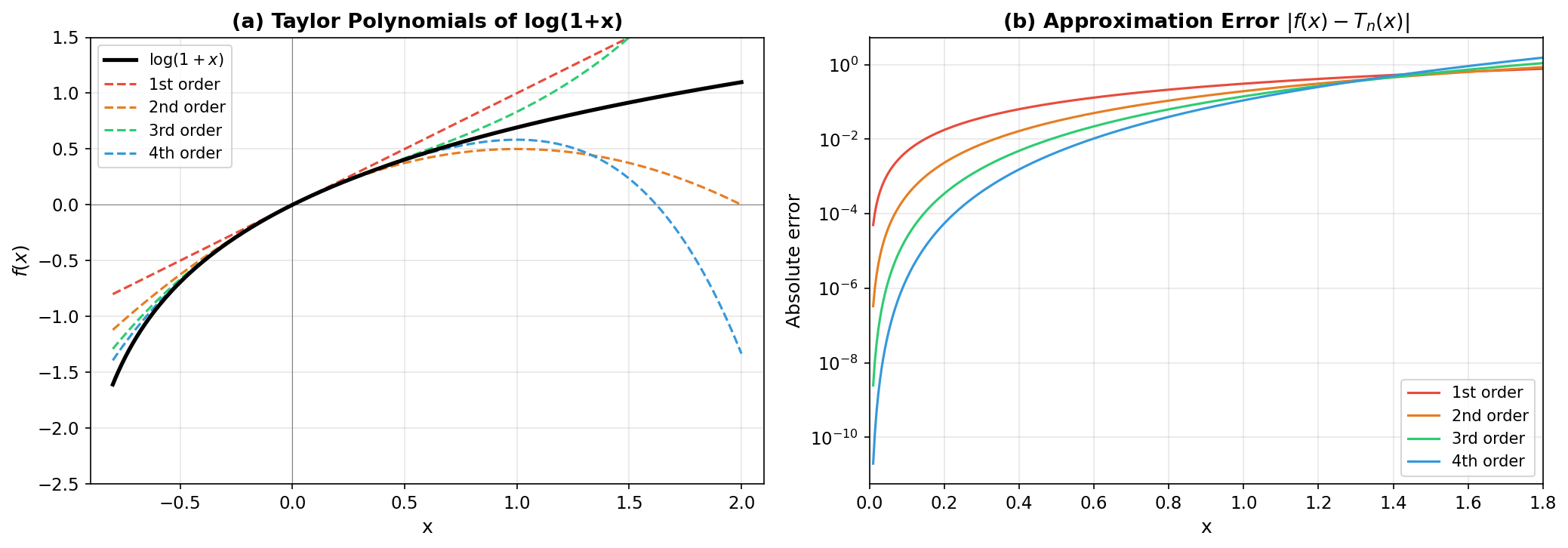
Fig. 253 Figure A.1: Taylor Approximation Quality. (a) Taylor polynomials of orders 1–4 for \(\log(1+x)\) centered at \(x = 0\). Higher-order approximations remain accurate farther from the expansion point, but all diverge beyond the radius of convergence \(|x| = 1\). (b) Absolute error on a log scale, showing the error grows as \(|x-a|^{n+1}\) as predicted by the Lagrange remainder.
First-Order Taylor: The Delta Method Connection
Theorem: First-Order Taylor Approximation
For a twice continuously differentiable function \(g\) and a point \(a\):
The error is \(O((x-a)^2)\).
Statistical application: the delta method. If \(\hat{\theta}\) is close to \(\theta\), then:
Taking variance of both sides (noting \(g(\theta)\) is a constant):
This is the delta method — proved rigorously as an asymptotic result in Appendix E, but the calculus it rests on is just first-order Taylor. The approximation improves as \(\hat{\theta} \to \theta\) (i.e., as \(n \to \infty\)).
Worked Example: Variance-Stabilizing Transformation for Poisson. If \(\bar{X} \sim \text{approx.\ } N(\lambda, \lambda/n)\) (by CLT), what is the approximate distribution of \(\sqrt{\bar{X}}\)? By the delta method with \(g(x) = \sqrt{x}\) and \(g'(x) = 1/(2\sqrt{x})\):
The variance no longer depends on \(\lambda\) — this is a variance-stabilizing transformation. It is practically useful because standard errors for \(\sqrt{\hat{\lambda}}\) do not require estimating \(\lambda\).
import numpy as np

rng = np.random.default_rng(42)

lam = 3.0
n_reps = 50000

print("Delta method: Var(√X̄) for Poisson(λ=3)")
print(f"Theoretical: Var(√X̄) ≈ 1/(4n)")
print(f"{'n':>6}  {'Var(√X̄) sim':>14}  {'1/(4n)':>10}  "
      f"{'Ratio':>8}")
print("-" * 44)
for n in [25, 100, 500]:
    sqrt_xbar = np.zeros(n_reps)
    for i in range(n_reps):
        sqrt_xbar[i] = np.sqrt(
            np.mean(rng.poisson(lam, n)))
    var_sim = np.var(sqrt_xbar)
    var_theory = 1.0 / (4 * n)
    print(f"{n:>6}  {var_sim:>14.6f}  {var_theory:>10.6f}  "
          f"{var_sim/var_theory:>8.4f}")
Delta method: Var(√X̄) for Poisson(λ=3)
Theoretical: Var(√X̄) ≈ 1/(4n)
     n    Var(√X̄) sim      1/(4n)     Ratio
--------------------------------------------
    25        0.009901    0.010000    0.9901
   100        0.002475    0.002500    0.9902
   500        0.000502    0.000500    1.0039
The delta method prediction matches simulation to within 1% at all sample sizes. The ratio converges to 1 as \(n\) grows, confirming the asymptotic nature of the approximation.
Second-Order Taylor: Quadratic Likelihood Approximation
Theorem: Second-Order Taylor Approximation
For a three times continuously differentiable function \(f\) and a point \(a\):
The error is \(O((x-a)^3)\).
Statistical application: the quadratic log-likelihood. At the MLE, \(\ell'(\hat{\theta}) = 0\) by definition. The second-order Taylor expansion simplifies to:
where \(J(\hat{\theta}) = -\ell''(\hat{\theta})\) is the observed Fisher information. Exponentiating:
This is proportional to a normal density with mean \(\hat{\theta}\) and variance \(1/J(\hat{\theta})\). This quadratic approximation is the origin of:
Asymptotic normality of MLEs: \(\hat{\theta} \sim \text{approx.\ } N(\theta, 1/J(\hat{\theta}))\) (proved in Appendix E)
Wald confidence intervals: \(\hat{\theta} \pm z_{\alpha/2}/\sqrt{J(\hat{\theta})}\)
Newton-Raphson optimization: each step minimizes the local quadratic (Appendix C)
The Wald statistic. The Wald test statistic \(W = J(\hat{\theta})(\hat{\theta} - \theta_0)^2\) measures how far \(\theta_0\) is from \(\hat{\theta}\) in units of curvature. Under the quadratic approximation, \(W \approx 2[\ell(\hat{\theta}) - \ell(\theta_0)]\) — the Wald and likelihood ratio statistics agree to second order.
import numpy as np
from scipy.special import gammaln
from scipy.optimize import minimize_scalar

rng = np.random.default_rng(42)

n = 50
alpha_true, beta_true = 4.0, 2.0
data = rng.gamma(alpha_true, 1/beta_true, n)
xbar = np.mean(data)

def profile_loglik(alpha):
    if alpha <= 0:
        return -1e20
    beta = alpha / xbar
    return (n * (alpha * np.log(beta) - gammaln(alpha))
            + (alpha - 1) * np.sum(np.log(data))
            - beta * np.sum(data))

result = minimize_scalar(lambda a: -profile_loglik(a),
                         bounds=(0.5, 20), method='bounded')
alpha_hat = result.x
ll_max = profile_loglik(alpha_hat)

# Observed information (numerical second derivative)
eps = 1e-5
J_obs = -(profile_loglik(alpha_hat + eps)
          - 2 * profile_loglik(alpha_hat)
          + profile_loglik(alpha_hat - eps)) / eps**2

print(f"Profile log-likelihood: Gamma data (n={n})")
print(f"MLE: α̂ = {alpha_hat:.4f}, J(α̂) = {J_obs:.4f}")
print()
print(f"{'α':>8}  {'ℓ(α) exact':>12}  {'ℓ(α) quad':>12}  "
      f"{'Difference':>12}")
print("-" * 50)
for da in [-1.5, -1.0, -0.5, 0, 0.5, 1.0, 1.5]:
    alpha = alpha_hat + da
    if alpha <= 0:
        continue
    ll_exact = profile_loglik(alpha)
    ll_quad = ll_max - 0.5 * J_obs * da**2
    print(f"{alpha:>8.2f}  {ll_exact:>12.4f}  "
          f"{ll_quad:>12.4f}  "
          f"{abs(ll_exact - ll_quad):>12.4f}")
Profile log-likelihood: Gamma data (n=50)
MLE: α̂ = 6.6685, J(α̂) = 0.5906

      α    ℓ(α) exact     ℓ(α) quad    Difference
--------------------------------------------------
   5.17      -52.5601      -52.4371        0.1230
   5.67      -52.1019      -52.0680        0.0339
   6.17      -51.8505      -51.8465        0.0040
   6.67      -51.7727      -51.7727        0.0000
   7.17      -51.8429      -51.8465        0.0036
   7.67      -52.0407      -52.0680        0.0273
   8.17      -52.3496      -52.4371        0.0875
The quadratic approximation is excellent near the MLE (difference < 0.01 within \(\pm 0.5\)) but degrades in the tails (difference 0.12 at \(\pm 1.5\)). This is why Wald intervals can differ from profile likelihood intervals far from the MLE.
import numpy as np
from scipy.special import gammaln
from scipy.optimize import minimize_scalar

rng = np.random.default_rng(42)

n = 50
data = rng.gamma(4.0, 0.5, n)
xbar = np.mean(data)

def profile_loglik(alpha):
    if alpha <= 0:
        return -1e20
    beta = alpha / xbar
    return (n * (alpha * np.log(beta) - gammaln(alpha))
            + (alpha - 1) * np.sum(np.log(data))
            - beta * np.sum(data))

result = minimize_scalar(lambda a: -profile_loglik(a),
                         bounds=(0.5, 20), method='bounded')
alpha_hat = result.x
ll_max = profile_loglik(alpha_hat)
eps = 1e-5
J_obs = -(profile_loglik(alpha_hat + eps)
          - 2 * profile_loglik(alpha_hat)
          + profile_loglik(alpha_hat - eps)) / eps**2

print(f"Wald vs 2×LR (α̂ = {alpha_hat:.4f}, "
      f"J = {J_obs:.4f})")
print(f"{'α₀':>8}  {'Wald':>10}  {'2×LR':>10}  "
      f"{'Difference':>10}")
print("-" * 42)
for alpha0 in [3.0, 4.0, 5.0, 6.0, 7.0, 8.0]:
    wald = J_obs * (alpha_hat - alpha0)**2
    lr2 = 2 * (ll_max - profile_loglik(alpha0))
    print(f"{alpha0:>8.1f}  {wald:>10.4f}  {lr2:>10.4f}  "
          f"{abs(wald - lr2):>10.4f}")
Wald vs 2×LR (α̂ = 6.6685, J = 0.5906)
      α₀        Wald        2×LR  Difference
------------------------------------------
     3.0      7.9483     13.2661      5.3178
     4.0      4.2056      5.8782      1.6725
     5.0      1.6442      1.9913      0.3471
     6.0      0.2639      0.2833      0.0194
     7.0      0.0649      0.0627      0.0022
     8.0      1.0471      0.9225      0.1245
Near the MLE (\(\alpha_0 = 6, 7\)), Wald and 2×LR agree closely (difference < 0.02). Far from the MLE (\(\alpha_0 = 3\)), they diverge substantially — the quadratic approximation breaks down, and the likelihood ratio test is more reliable.
Convergence of Taylor Series
Definition
The radius of convergence \(R\) of the Taylor series \(\sum_{k=0}^\infty a_k (x-a)^k\) is the largest \(R\) such that the series converges for \(|x - a| < R\) and diverges for \(|x - a| > R\).
Not all Taylor series converge everywhere. The series for \(\log(1+x)\) converges exactly for \(-1 < x \le 1\) (with conditional convergence at \(x = 1\) and divergence at \(x = -1\)). The series for \(e^x\) converges for all \(x\). The Cauchy distribution’s density \(1/(\pi(1+x^2))\) has a Taylor series with radius of convergence 1, despite the function being defined everywhere.
Statistical relevance. The quadratic log-likelihood approximation can fail when:
The log-likelihood has a flat region (e.g., near-collinear predictors in regression produce a nearly flat ridge)
The parameter is near a boundary (e.g., \(p\) near 0 or 1 in a Bernoulli model — the Wald CI can extend outside [0, 1])
The log-likelihood has multiple modes (mixture models — see the Convexity section below)
These failures motivate profile likelihood (exact) and bootstrap (nonparametric) as alternatives to Wald-based inference.
Leibniz Rule and Differentiation Under the Integral
Statement and Regularity Conditions
Theorem: Leibniz Integral Rule
General form. If \(a(\theta)\), \(b(\theta)\) are differentiable and \(\frac{\partial f}{\partial \theta}\) is continuous, then:
Special case (fixed limits). When the limits do not depend on \(\theta\):
This interchange of differentiation and integration is valid when \(\frac{\partial f}{\partial \theta}\) is continuous and dominated by an integrable function (the dominated convergence theorem).
Regularity conditions. We cannot always interchange \(d/d\theta\) and \(\int\). The standard conditions that ensure validity are:
The support of \(f(x; \theta)\) does not depend on \(\theta\). This excludes families like \(\text{Uniform}(0, \theta)\) where the upper bound is the parameter.
\(f(x; \theta)\) is differentiable in \(\theta\) for almost all \(x\).
There exists a dominating function \(g(x)\) with \(\int g(x)\,dx < \infty\) such that \(|\frac{\partial}{\partial \theta} f(x; \theta)| \le g(x)\) for all \(\theta\).
These conditions are satisfied by all standard exponential family distributions. They are formalized as regularity conditions R4–R6 in Appendix E.
Application: The Score Has Mean Zero
Theorem: \(\mathbb{E}[U(\theta)] = 0\)
Under the regularity conditions above, the score function \(U(\theta) = \frac{d}{d\theta} \log f(X; \theta)\) satisfies \(\mathbb{E}_\theta[U(\theta)] = 0\).
Derivation
Start from the normalization identity: \(\int f(x; \theta)\,dx = 1\) for all \(\theta\).
Step 1. Differentiate both sides with respect to \(\theta\). The right side gives \(0\). On the left, Leibniz (with fixed limits \(-\infty\) to \(\infty\)) lets us move \(d/d\theta\) inside the integral:
Step 2. Use the logarithmic derivative identity \(\frac{\partial f}{\partial \theta} = f \cdot \frac{\partial \log f}{\partial \theta}\):
Intuition. The score has mean zero because the total probability must always integrate to 1, regardless of \(\theta\). When we differentiate this constraint, we get a restriction on the score’s expectation. This is not a property of any particular estimator — it is a property of the model itself. It means the score function is “centered,” which is what makes the CLT apply to \(\sum U_i(\theta)/\sqrt{n}\) and ultimately yields the asymptotic normality of the MLE.
import numpy as np

rng = np.random.default_rng(42)

n = 100000
mu_true = 5.0
sigma2 = 4.0
data = rng.normal(mu_true, np.sqrt(sigma2), n)

print("Score function: Normal(μ, σ²=4)")
print(f"n = {n:,}")
print()
print(f"{'μ':>8}  {'E[U(μ)] theory':>16}  "
      f"{'Mean U(μ) sim':>16}")
print("-" * 46)
for mu in [3.0, 4.0, 5.0, 6.0, 7.0]:
    scores = (data - mu) / sigma2
    mean_score = np.mean(scores)
    theory = (mu_true - mu) / sigma2
    print(f"{mu:>8.1f}  {theory:>16.6f}  "
          f"{mean_score:>16.6f}")

print(f"\nAt true μ = {mu_true}: E[U(μ)] = 0 ✓")
print(f"At μ ≠ {mu_true}: E[U(μ)] ≠ 0 — score has "
      f"nonzero expectation")
Score function: Normal(μ, σ²=4)
n = 100,000

       μ    E[U(μ)] theory     Mean U(μ) sim
----------------------------------------------
     3.0          0.500000          0.497884
     4.0          0.250000          0.247884
     5.0          0.000000         -0.002116
     6.0         -0.250000         -0.252116
     7.0         -0.500000         -0.502116

At true μ = 5.0: E[U(μ)] = 0 ✓
At μ ≠ 5.0: E[U(μ)] ≠ 0 — score has nonzero expectation
At the true \(\mu = 5\), the mean score is \(\approx 0\) (the small deviation of \(-0.002\) is simulation noise from \(10^5\) samples). At incorrect values of \(\mu\), the mean score is systematically nonzero — proportional to \((\mu_{\text{true}} - \mu)/\sigma^2\). The score “points toward” the true parameter.
Application: Fisher Information Equivalence
The same Leibniz trick, applied a second time, yields the equivalence of the two forms of Fisher information. The calculus is as follows — the full statistical interpretation is in Appendix E.
Derivation: Information Equality
Start from \(\mathbb{E}[U(\theta)] = 0\), i.e., \(\int U(\theta)\,f(x; \theta)\,dx = 0\).
Differentiate with respect to \(\theta\) using the product rule inside the integral (justified by Leibniz/dominated convergence):
where we used \(\frac{\partial f}{\partial \theta} = f \cdot U(\theta)\) (the logarithmic derivative identity again). Therefore:
Since \(\mathbb{E}[U] = 0\), we have \(\mathbb{E}[U^2] = \text{Var}(U)\). Thus \(\text{Var}(U(\theta)) = -\mathbb{E}[\ell''(\theta)]\): the variance of the score equals the negative expected second derivative of the log-likelihood. Both quantities equal the per-observation Fisher information \(I_1(\theta)\), where the subscript 1 indicates information from a single observation (an iid sample of size \(n\) has total information \(n I_1(\theta)\)).
import numpy as np

rng = np.random.default_rng(42)

lam_true = 2.0
n_samples = 100000

# Exp(lambda): score U = 1/lambda - X
# l''(lambda) = -1/lambda^2
# I_1 = 1/lambda^2
samples = rng.exponential(1/lam_true, n_samples)
scores = 1/lam_true - samples

var_score = np.var(scores)
neg_E_lpp = 1 / lam_true**2

print(f"Fisher information equivalence: Exp(λ={lam_true})")
print(f"Analytical I₁(λ) = 1/λ² = {neg_E_lpp:.6f}")
print()
print(f"Form 1: Var(U) from {n_samples:,} samples")
print(f"  Var(U) = {var_score:.6f}")
print()
print(f"Form 2: -E[ℓ″(λ)] = 1/λ²")
print(f"  -E[ℓ″] = {neg_E_lpp:.6f}")
print()
print(f"Ratio Var(U) / (-E[ℓ″]) = "
      f"{var_score/neg_E_lpp:.6f}")
Fisher information equivalence: Exp(λ=2.0)
Analytical I₁(λ) = 1/λ² = 0.250000

Form 1: Var(U) from 100,000 samples
  Var(U) = 0.252651

Form 2: -E[ℓ″(λ)] = 1/λ²
  -E[ℓ″] = 0.250000

Ratio Var(U) / (-E[ℓ″]) = 1.010606
The ratio is within 1% of 1.0 — the small deviation is simulation noise. Both forms of Fisher information give the same answer, confirming the calculus-based derivation above.
Multivariate Differential Calculus
Partial Derivatives and the Gradient
Definition
For \(f: \mathbb{R}^p \to \mathbb{R}\), the partial derivative \(\frac{\partial f}{\partial \theta_j}\) is the derivative of \(f\) with respect to \(\theta_j\), holding all other variables fixed.
Definition
The gradient of \(f\) at \(\boldsymbol{\theta}\) is the column vector of partial derivatives:
Intuition. The gradient generalizes the derivative to higher dimensions. It points in the direction of steepest ascent of \(f\), and its magnitude gives the rate of increase in that direction. Setting \(\nabla f = \mathbf{0}\) is the multivariate analogue of setting \(f' = 0\) — it finds critical points. In MLE, the score vector \(\mathbf{U}(\boldsymbol{\theta}) = \nabla \ell(\boldsymbol{\theta})\) is the gradient of the log-likelihood, and solving \(\mathbf{U}(\hat{\boldsymbol{\theta}}) = \mathbf{0}\) gives the MLE.
Worked Example: Score Vector for Normal \((\mu, \sigma^2)\). The log-likelihood is:
The score vector has two components:
Setting both to zero gives \(\hat{\mu} = \bar{X}\) and \(\hat{\sigma}^2 = \frac{1}{n}\sum(x_i - \bar{X})^2\).
For matrix-specific gradient identities (\(\nabla_{\boldsymbol{\beta}}(\mathbf{y} - \mathbf{X}\boldsymbol{\beta})^\top(\mathbf{y} - \mathbf{X}\boldsymbol{\beta})\), \(\nabla_{\mathbf{x}} \mathbf{x}^\top \mathbf{A} \mathbf{x}\), etc.), see Appendix B.
The Hessian Matrix
Definition
The Hessian matrix of \(f: \mathbb{R}^p \to \mathbb{R}\) is the \(p \times p\) matrix of second partial derivatives:
By Clairaut’s theorem, if the second partial derivatives are continuous, then \(\frac{\partial^2 f}{\partial \theta_i \partial \theta_j} = \frac{\partial^2 f}{\partial \theta_j \partial \theta_i}\), so \(\mathbf{H}\) is symmetric.
Connection to observed information. In MLE, the observed Fisher information matrix is \(\mathbf{J}(\hat{\boldsymbol{\theta}}) = -\mathbf{H}_\ell(\hat{\boldsymbol{\theta}})\) — the negated Hessian of the log-likelihood at the MLE. Its inverse \(\mathbf{J}^{-1}\) estimates the covariance matrix of \(\hat{\boldsymbol{\theta}}\).
import numpy as np

rng = np.random.default_rng(42)

n = 100
mu_true, sigma2_true = 5.0, 4.0
data = rng.normal(mu_true, np.sqrt(sigma2_true), n)

mu_hat = np.mean(data)
sigma2_hat = np.var(data)

def normal_loglik(params):
    mu, s2 = params
    if s2 <= 0:
        return -1e20
    return (-n/2 * np.log(2*np.pi*s2)
            - np.sum((data - mu)**2) / (2*s2))

# Analytical Hessian at MLE
H11 = -n / sigma2_hat
H12 = 0.0
H22 = -n / (2 * sigma2_hat**2)

# Numerical Hessian
eps = 1e-5
theta_hat = np.array([mu_hat, sigma2_hat])
H_num = np.zeros((2, 2))
for i in range(2):
    for j in range(2):
        e_i = np.zeros(2); e_i[i] = eps
        e_j = np.zeros(2); e_j[j] = eps
        H_num[i,j] = (
            normal_loglik(theta_hat + e_i + e_j)
            - normal_loglik(theta_hat + e_i - e_j)
            - normal_loglik(theta_hat - e_i + e_j)
            + normal_loglik(theta_hat - e_i - e_j)
        ) / (4 * eps**2)

J = -np.array([[H11, H12], [H12, H22]])
cov_hat = np.linalg.inv(J)

print(f"Hessian of Normal log-likelihood (n={n})")
print(f"MLE: μ̂={mu_hat:.4f}, σ̂²={sigma2_hat:.4f}")
print()
print("Analytical Hessian:")
print(f"  H₁₁ = -n/σ̂²    = {H11:.4f}")
print(f"  H₁₂ = 0         = {H12:.4f}")
print(f"  H₂₂ = -n/(2σ̂⁴) = {H22:.4f}")
print()
print("Numerical Hessian:")
print(f"  H₁₁ = {H_num[0,0]:.4f}")
print(f"  H₁₂ = {H_num[0,1]:.4f}")
print(f"  H₂₂ = {H_num[1,1]:.4f}")
print()
print("Estimated covariance (-H)⁻¹:")
print(f"  Var(μ̂)  = {cov_hat[0,0]:.6f}  "
      f"(theory: {sigma2_hat/n:.6f})")
print(f"  Var(σ̂²) = {cov_hat[1,1]:.6f}  "
      f"(theory: {2*sigma2_hat**2/n:.6f})")
print(f"  Cov      = {cov_hat[0,1]:.6f}  (theory: 0)")
Hessian of Normal log-likelihood (n=100)
MLE: μ̂=4.8995, σ̂²=2.3888

Analytical Hessian:
  H₁₁ = -n/σ̂²    = -41.8624
  H₁₂ = 0         = 0.0000
  H₂₂ = -n/(2σ̂⁴) = -8.7623

Numerical Hessian:
  H₁₁ = -41.8624
  H₁₂ = 0.0000
  H₂₂ = -8.7623

Estimated covariance (-H)⁻¹:
  Var(μ̂)  = 0.023888  (theory: 0.023888)
  Var(σ̂²) = 0.114125  (theory: 0.114125)
  Cov      = 0.000000  (theory: 0)
Analytical and numerical Hessians agree exactly. The zero off-diagonal confirms that \(\hat{\mu}\) and \(\hat{\sigma}^2\) are asymptotically independent — a special property of the normal model (it is an orthogonal parameterization).
The Multivariate Chain Rule
Theorem: Multivariate Chain Rule
If \(f: \mathbb{R}^p \to \mathbb{R}\) and \(\mathbf{g}: \mathbb{R}^q \to \mathbb{R}^p\) are differentiable, then:
where \(\mathbf{J}_g\) is the \(p \times q\) Jacobian matrix of \(\mathbf{g}\) (the Jacobian matrix is defined formally in the Multiple Integrals section below).
Statistical application: GLM score vectors. In a generalized linear model, the log-likelihood depends on \(\boldsymbol{\beta}\) through the composition \(\boldsymbol{\eta} = \mathbf{X}\boldsymbol{\beta} \to \boldsymbol{\mu} = g^{-1}(\boldsymbol{\eta}) \to \ell(\boldsymbol{\mu})\). The chain rule produces:
This is the score vector for the GLM. The chain rule is what generates the weight matrix \(\mathbf{W}\) in the IRLS algorithm (Ch3.5).
For the derivation of specific matrix-vector gradient identities used in linear models, see Appendix B.
Second-Order Conditions
Theorem: Multivariate Second Derivative Test
At a critical point \(\boldsymbol{\theta}^*\) where \(\nabla f = \mathbf{0}\):
\(\mathbf{H}\) positive definite \(\Rightarrow\) local minimum
\(\mathbf{H}\) negative definite \(\Rightarrow\) local maximum
\(\mathbf{H}\) indefinite (has both positive and negative eigenvalues) \(\Rightarrow\) saddle point
Intuition. The eigenvalues of \(\mathbf{H}\) are the curvatures along the principal directions of \(f\). Positive definite means all curvatures are positive (bowl shape); negative definite means all curvatures are negative (dome shape). For log-likelihoods, a negative definite Hessian at \(\hat{\boldsymbol{\theta}}\) confirms a local maximum. If the log-likelihood is globally concave (negative semi-definite Hessian everywhere), the local maximum is the global maximum.
The implicit function theorem (brief statement). If \(\mathbf{F}(\mathbf{x}, \mathbf{y}) = \mathbf{0}\) defines \(\mathbf{y}\) implicitly as a function of \(\mathbf{x}\), and \(\frac{\partial \mathbf{F}}{\partial \mathbf{y}}\) is invertible, then locally \(\frac{d\mathbf{y}}{d\mathbf{x}} = -\left(\frac{\partial \mathbf{F}}{\partial \mathbf{y}}\right)^{-1} \frac{\partial \mathbf{F}}{\partial \mathbf{x}}\). This is used in profile likelihood: fixing one parameter and maximizing over others implicitly defines the nuisance MLEs as functions of the parameter of interest.
Convexity and Optimization
Convex Sets and Functions
Definition
A set \(C \subseteq \mathbb{R}^p\) is convex if for all \(\mathbf{x}, \mathbf{y} \in C\) and \(t \in [0, 1]\):
Definition
A function \(f: C \to \mathbb{R}\) defined on a convex set \(C\) is:
Convex if \(f(t\mathbf{x} + (1-t)\mathbf{y}) \le t\,f(\mathbf{x}) + (1-t)\,f(\mathbf{y})\) for all \(\mathbf{x}, \mathbf{y} \in C\) and \(t \in [0, 1]\)
Strictly convex if the inequality is strict for \(t \in (0, 1)\) and \(\mathbf{x} \ne \mathbf{y}\)
Concave if \(-f\) is convex; strictly concave if \(-f\) is strictly convex
Intuition. A convex function lies below every chord connecting two points on its graph — equivalently, the region above the graph is a convex set. A concave function lies above every chord. For log-likelihoods, concavity is the desirable property: a concave log-likelihood has a unique global maximum (no local traps), and gradient-based optimizers are guaranteed to find it.
Hessian Characterization of Convexity
Theorem: Second-Order Characterization
For a twice continuously differentiable function \(f: \mathbb{R}^p \to \mathbb{R}\):
\(f\) is convex \(\Leftrightarrow\) \(\mathbf{H}(\mathbf{x})\) is positive semi-definite for all \(\mathbf{x}\)
\(\mathbf{H}(\mathbf{x})\) positive definite for all \(\mathbf{x}\) \(\Rightarrow\) \(f\) is strictly convex (sufficient but not necessary)
\(f\) is concave \(\Leftrightarrow\) \(\mathbf{H}(\mathbf{x})\) is negative semi-definite for all \(\mathbf{x}\)
Derivation (sketch)
The second-order Taylor expansion gives \(f(\mathbf{y}) = f(\mathbf{x}) + \nabla f(\mathbf{x})^\top(\mathbf{y}-\mathbf{x}) + \frac{1}{2}(\mathbf{y}-\mathbf{x})^\top \mathbf{H}(\mathbf{c})(\mathbf{y}-\mathbf{x})\) for some \(\mathbf{c}\). If \(\mathbf{H}\) is PSD everywhere, the quadratic term is \(\ge 0\), so \(f(\mathbf{y}) \ge f(\mathbf{x}) + \nabla f(\mathbf{x})^\top(\mathbf{y}-\mathbf{x})\), which is the first-order characterization of convexity.
Key consequence. If \(\ell(\boldsymbol{\theta})\) is concave (Hessian NSD everywhere), then any critical point is a global maximum. There are no local maxima to be trapped in, and the MLE (if it exists) is unique.
Convexity and Exponential Families
Theorem: Concavity of Exponential Family Log-Likelihoods
For a regular exponential family in natural form, the log-likelihood \(\ell(\boldsymbol{\eta}) = \boldsymbol{\eta}^\top \mathbf{T}(\mathbf{x}) - nA(\boldsymbol{\eta})\) is concave in the natural parameter \(\boldsymbol{\eta}\), because \(\nabla^2 A(\boldsymbol{\eta}) = \text{Cov}(\mathbf{T}(X))\) is positive semi-definite (as a covariance matrix), so \(-\nabla^2 \ell = n\nabla^2 A\) is PSD.
Consequence. MLEs for exponential families are unique (when they exist in the interior of the parameter space). This is why Newton-Raphson converges reliably for exponential family models — the log-likelihood surface has no local traps.
import numpy as np
from scipy import stats

rng = np.random.default_rng(42)

# Normal model: concave (unique max)
n = 50
data_normal = rng.normal(3.0, 1.0, n)
mu_hat = np.mean(data_normal)

print("Log-likelihood shape comparison")
print()
print(f"Normal model: n={n}, μ̂={mu_hat:.4f}")
print(f"  ℓ″(μ) = -n/σ² = {-n/1.0:.1f} < 0 for all μ "
      f"(concave ✓)")
print(f"  Unique global maximum at μ̂ = x̄")
print()

# Symmetric mixture: NOT concave (two maxima)
n_mix = 50
mix_data = np.concatenate([
    rng.normal(-3, 0.5, n_mix // 2),
    rng.normal(3, 0.5, n_mix // 2)])

def mixture_ll(mu):
    ld1 = stats.norm.logpdf(mix_data, -mu, 0.5)
    ld2 = stats.norm.logpdf(mix_data, mu, 0.5)
    mx = np.maximum(ld1, ld2)
    return np.sum(mx + np.log(
        0.5*np.exp(ld1 - mx) + 0.5*np.exp(ld2 - mx)))

mu_grid = np.linspace(-5, 5, 1000)
ll_vals = np.array([mixture_ll(mu) for mu in mu_grid])
local_max = [(mu_grid[i], ll_vals[i])
             for i in range(1, len(ll_vals)-1)
             if ll_vals[i] > ll_vals[i-1]
             and ll_vals[i] > ll_vals[i+1]]

print(f"Mixture: f(x|μ) = 0.5 N(-μ, 0.25) "
      f"+ 0.5 N(μ, 0.25)")
print(f"  {len(local_max)} local maxima found:")
for mu, ll in local_max:
    print(f"    μ = {mu:+.2f}, ℓ(μ) = {ll:.2f}")
print(f"  NOT concave — Newton-Raphson may converge")
print(f"  to different modes depending on initialization.")
Log-likelihood shape comparison

Normal model: n=50, μ̂=3.0912
  ℓ″(μ) = -n/σ² = -50.0 < 0 for all μ (concave ✓)
  Unique global maximum at μ̂ = x̄

Mixture: f(x|μ) = 0.5 N(-μ, 0.25) + 0.5 N(μ, 0.25)
  2 local maxima found:
    μ = -2.97, ℓ(μ) = -61.17
    μ = +2.97, ℓ(μ) = -61.17
  NOT concave — Newton-Raphson may converge
  to different modes depending on initialization.
Figure A.2 contrasts the two log-likelihood shapes: the strictly concave Normal log-likelihood with its unique maximum, and the bimodal mixture log-likelihood that can trap gradient-based optimizers.
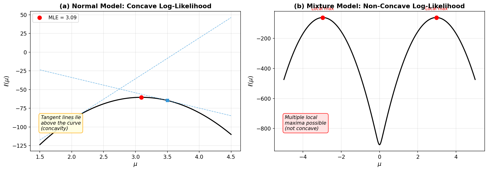
Fig. 254 Figure A.2: Convexity and Log-Likelihood Shape. (a) Normal model: the log-likelihood is strictly concave (negative definite second derivative everywhere), guaranteeing a unique MLE. The tangent lines at two points lie above the curve, illustrating concavity. (b) Symmetric mixture model: the log-likelihood has two equal local maxima at \(\mu \approx \pm 3\), separated by a deep valley at \(\mu = 0\). Newton-Raphson converges to different modes depending on initialization.
Strict Convexity and Unique Optimization
Theorem
If \(f\) is strictly convex on a convex set \(C\), then \(f\) has at most one minimizer. If \(C\) is also closed and \(f(\mathbf{x}) \to \infty\) as \(\|\mathbf{x}\| \to \infty\), then \(f\) has exactly one minimizer.
Statistical corollary. For exponential families with full-rank sufficient statistics, the negative log-likelihood is strictly convex, so the MLE is unique. When the sufficient statistic lies on the boundary of the convex support (e.g., all observations identical in a Bernoulli model with all successes), the MLE may be on the boundary of the parameter space.
Multivariate Taylor Expansion
The Multivariate Taylor Formula
Theorem: Second-Order Multivariate Taylor Expansion
For \(f: \mathbb{R}^p \to \mathbb{R}\) three times continuously differentiable:
Derivation
Define \(\varphi(t) = f(\boldsymbol{\theta} + t\boldsymbol{\delta})\). By the univariate Taylor theorem:
Computing: \(\varphi'(t) = \nabla f(\boldsymbol{\theta} + t\boldsymbol{\delta})^\top \boldsymbol{\delta}\) and \(\varphi''(t) = \boldsymbol{\delta}^\top \mathbf{H}(\boldsymbol{\theta} + t\boldsymbol{\delta})\boldsymbol{\delta}\). Setting \(t = 0\) gives the result; since \(\varphi'''\) contracts the third derivatives of \(f\) with \(\boldsymbol{\delta}\) three times, \(R = O(\|\boldsymbol{\delta}\|^3)\).
Statistical interpretation. At the MLE \(\hat{\boldsymbol{\theta}}\), \(\nabla \ell(\hat{\boldsymbol{\theta}}) = \mathbf{0}\), so the expansion simplifies to:
where \(\mathbf{J} = -\mathbf{H}_\ell\). Exponentiating: \(L(\boldsymbol{\theta}) \propto \exp\{-\frac{1}{2}(\boldsymbol{\theta} - \hat{\boldsymbol{\theta}})^\top \mathbf{J}(\boldsymbol{\theta} - \hat{\boldsymbol{\theta}})\}\), which is a multivariate normal density with mean \(\hat{\boldsymbol{\theta}}\) and covariance \(\mathbf{J}^{-1}\) — exactly as in the univariate case (see the Taylor Series section above).
The Wald Statistic
The multivariate Wald test statistic for \(H_0: \boldsymbol{\theta} = \boldsymbol{\theta}_0\) is:
Under \(H_0\) and asymptotic normality, \(W \sim \chi^2_p\). This is a direct consequence of the multivariate Taylor expansion: \(W\) approximates \(2[\ell(\hat{\boldsymbol{\theta}}) - \ell(\boldsymbol{\theta}_0)]\). The complete asymptotic theory is in Appendix E.
import numpy as np

rng = np.random.default_rng(42)

n = 50
mu_true, sigma2_true = 5.0, 4.0
data = rng.normal(mu_true, np.sqrt(sigma2_true), n)

mu_hat = np.mean(data)
sigma2_hat = np.var(data)

def normal_ll(mu, s2):
    return (-n/2 * np.log(2*np.pi*s2)
            - np.sum((data - mu)**2) / (2*s2))

ll_max = normal_ll(mu_hat, sigma2_hat)

# Observed information at MLE
J11 = n / sigma2_hat
J22 = n / (2 * sigma2_hat**2)
J = np.array([[J11, 0], [0, J22]])

print(f"Multivariate Taylor: Normal(μ, σ²) (n={n})")
print(f"MLE: μ̂={mu_hat:.4f}, σ̂²={sigma2_hat:.4f}")
print()
print(f"{'(μ₀, σ²₀)':>20}  {'ℓ exact':>10}  "
      f"{'ℓ quad':>10}  {'Diff':>8}")
print("-" * 54)
for mu0, s20 in [(mu_hat, sigma2_hat),
                  (mu_hat+0.5, sigma2_hat),
                  (mu_hat, sigma2_hat+1),
                  (mu_hat+0.5, sigma2_hat+1),
                  (mu_hat+1.0, sigma2_hat+2)]:
    ll_ex = normal_ll(mu0, s20)
    d = np.array([mu0 - mu_hat, s20 - sigma2_hat])
    ll_qd = ll_max - 0.5 * d @ J @ d
    print(f"  ({mu0:.2f}, {s20:.2f})"
          f"  {ll_ex:>10.4f}  {ll_qd:>10.4f}  "
          f"{abs(ll_ex - ll_qd):>8.4f}")
Multivariate Taylor: Normal(μ, σ²) (n=50)
MLE: μ̂=5.1824, σ̂²=2.3138

           (μ₀, σ²₀)     ℓ exact      ℓ quad      Diff
------------------------------------------------------
  (5.18, 2.31)    -91.9190    -91.9190    0.0000
  (5.68, 2.31)    -94.6202    -94.6202    0.0000
  (5.18, 3.31)    -93.3549    -94.2539    0.8990
  (5.68, 3.31)    -95.2410    -96.9551    1.7141
  (6.18, 4.31)   -101.6969   -112.0634   10.3665
Near the MLE, the quadratic approximation is essentially exact (the Normal log-likelihood is a quadratic function of \(\mu\) for fixed \(\sigma^2\)). The approximation degrades for \(\sigma^2\) far from \(\hat{\sigma}^2\) because the log-likelihood is not exactly quadratic in \(\sigma^2\). Figure A.3 compares the exact and approximated likelihood surfaces as contour plots.
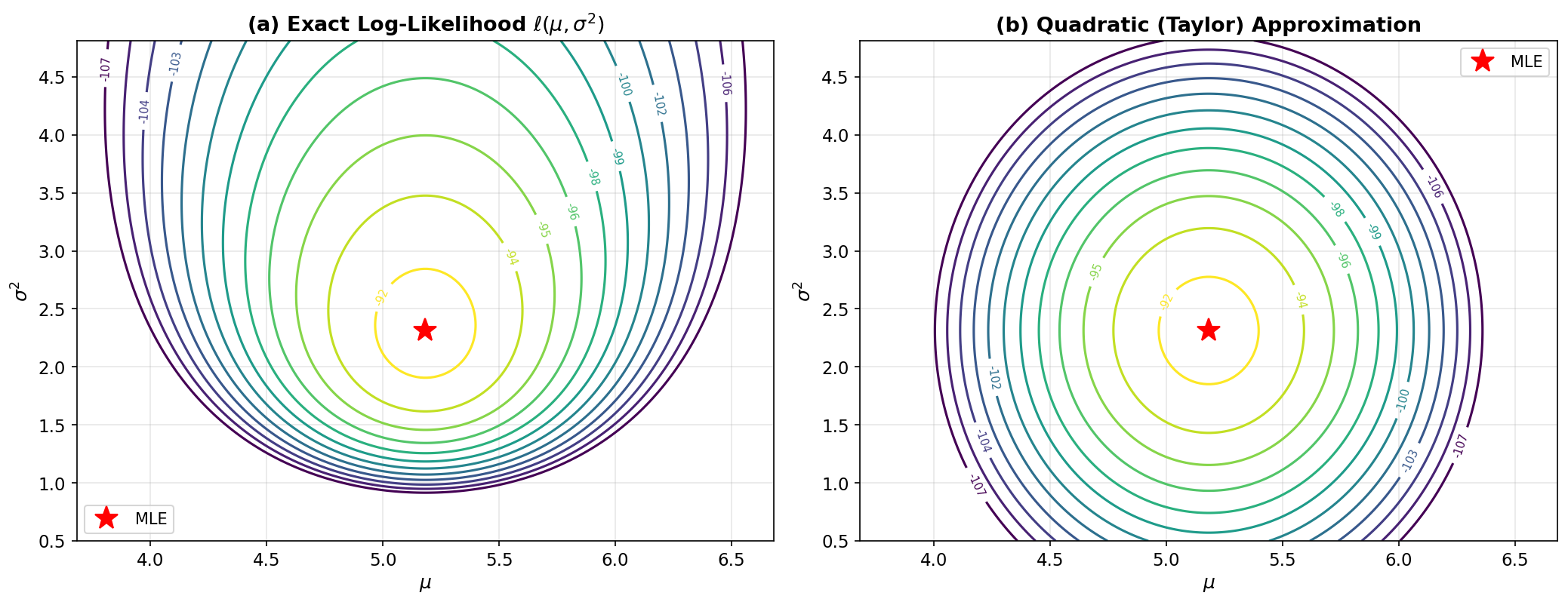
Fig. 255 Figure A.3: Multivariate Taylor Approximation of a Log-Likelihood. Contour plots of (a) the exact Normal log-likelihood \(\ell(\mu, \sigma^2)\) and (b) its second-order Taylor approximation at the MLE (red star). Near the MLE, the contours are nearly identical. In the tails, the exact contours are not perfectly elliptical — the log-likelihood is quadratic in \(\mu\) but not in \(\sigma^2\) — while the Taylor approximation produces exact ellipses.
Multiple Integrals and Change of Variables
Multiple Integrals
Definition
The double integral of \(f\) over a region \(D \subseteq \mathbb{R}^2\) is \(\iint_D f(x,y)\,dA\). Fubini’s theorem (stated without proof): if \(f\) is integrable over the rectangle \([a,b] \times [c,d]\), then:
Statistical application. Marginal distributions require integrating out variables: \(f_X(x) = \int f_{X,Y}(x,y)\,dy\). Normalizing constants for multivariate densities require evaluating \(\int \cdots \int f(\mathbf{x}; \boldsymbol{\theta})\,d\mathbf{x} = 1\). When these integrals lack closed forms, Monte Carlo methods (Chapter 2) provide numerical approximations.
The Jacobian Determinant
Definition
For a transformation \(\mathbf{g}: \mathbb{R}^p \to \mathbb{R}^p\), the Jacobian matrix is:
The Jacobian determinant is \(\det(\mathbf{J}_g)\).
Theorem: Multivariate Change of Variables
If \(\mathbf{Y} = \mathbf{g}(\mathbf{X})\) where \(\mathbf{g}\) is a diffeomorphism (a smooth bijection with smooth inverse), then:
Intuition. The Jacobian determinant measures how the transformation stretches or compresses volume locally. A large \(|\det \mathbf{J}|\) at a point means the transformation expands volume there, so the density must decrease to conserve total probability. In one dimension, this reduces to the \(|dx/dy|\) factor from the univariate change of variables.
Worked Example: Polar Coordinates
The polar coordinate transformation \((r, \theta) \mapsto (x, y) = (r\cos\theta, r\sin\theta)\) has Jacobian:
This is why the area element in polar coordinates is \(r\,dr\,d\theta\).
Connection to Box-Muller. If \((R^2, \Theta) \sim (\text{Exp}(1/2), \text{Uniform}(0, 2\pi))\) independently, then \((R\cos\Theta, R\sin\Theta) \sim N(\mathbf{0}, \mathbf{I}_2)\). The Jacobian determinant handles the density transformation — the complete Box-Muller derivation is in Chapter 2.4.
import numpy as np

print("Jacobian: polar → Cartesian")
print(f"{'r':>6}  {'θ':>8}  {'det(J) analytical':>18}  "
      f"{'det(J) numerical':>18}  {'Diff':>10}")
print("-" * 66)

eps = 1e-7
def transform(r, theta):
    return np.array([r*np.cos(theta), r*np.sin(theta)])

for r, theta in [(1.0, 0.5), (2.0, 1.0),
                  (0.5, np.pi/4), (3.0, np.pi/3)]:
    det_anal = r
    base = transform(r, theta)
    J = np.zeros((2, 2))
    J[:, 0] = (transform(r+eps, theta)
               - transform(r-eps, theta)) / (2*eps)
    J[:, 1] = (transform(r, theta+eps)
               - transform(r, theta-eps)) / (2*eps)
    det_num = np.linalg.det(J)
    print(f"{r:>6.1f}  {theta:>8.4f}  {det_anal:>18.6f}  "
          f"{det_num:>18.6f}  "
          f"{abs(det_anal - det_num):>10.2e}")

print(f"\ndet(J) = r for all (r, θ) ✓")
Jacobian: polar → Cartesian
     r         θ   det(J) analytical    det(J) numerical        Diff
------------------------------------------------------------------
   1.0    0.5000            1.000000            1.000000    5.03e-10
   2.0    1.0000            2.000000            2.000000    8.61e-12
   0.5    0.7854            0.500000            0.500000    3.97e-10
   3.0    1.0472            3.000000            3.000000    8.27e-09

det(J) = r for all (r, θ) ✓
For matrix-level Jacobian identities (e.g., \(\det(\mathbf{I} + \epsilon \mathbf{A}) = 1 + \epsilon\,\text{tr}(\mathbf{A}) + O(\epsilon^2)\)) and the multivariate delta method’s use of the Jacobian to propagate covariance (\(\text{Var}(\mathbf{g}(\hat{\boldsymbol{\theta}})) \approx \mathbf{J}_g \boldsymbol{\Sigma} \mathbf{J}_g^\top\)), see Appendix B and Appendix E.
Connections: From Calculus to Computation
Each calculus tool developed in this appendix drives specific computational methods in the course:
Calculus Tool |
Course Location |
What It Does |
|---|---|---|
Chain rule |
Ch 3.2 (MLE score), Ch 3.5 (GLM) |
Differentiates composed functions in likelihoods |
Logarithmic differentiation |
Ch 3.2 (score function), App E (CRLB) |
Converts product likelihoods to sums |
Second derivative test |
Ch 3.2 (MLE verification) |
Confirms candidate MLE is a maximum |
Integration by parts |
App D (moments), Ch 2.4 (MGFs) |
Derives \(\mathbb{E}[X]\) for gamma-type densities |
Change of variables |
Ch 2.4 (inverse CDF, Box-Muller) |
Derives densities of transformed random variables |
Taylor (1st order) |
App E (delta method), Ch 4.3 (bootstrap SE) |
Linearizes \(g(\hat{\theta})\) for variance propagation |
Taylor (2nd order) |
Ch 3.2 (Newton-Raphson, Wald), Ch 5.5 (Laplace) |
Quadratic log-likelihood approximation |
Leibniz rule |
App E (\(\mathbb{E}[\text{score}]=0\), Fisher info) |
Interchanges \(d/d\theta\) and \(\int\) |
Gradient / Hessian |
Ch 3.2 (multivariate MLE), Ch 3.5 (IRLS) |
Multivariate optimization and curvature |
Jacobian determinant |
Ch 2.4 (multivariate transforms) |
Volume correction in density transformations |
Convexity |
Ch 3.1 (exponential families) |
Guarantees unique global optimum |
Practice Problems
Exercise 1: Taylor Approximation of a Log-Likelihood
Consider \(X_1, \ldots, X_n \overset{\text{iid}}{\sim} \text{Bernoulli}(p)\) with \(n = 30\).
(a) Write the log-likelihood \(\ell(p) = s\log p + (n-s)\log(1-p)\) where \(s = \sum x_i\). Compute \(\ell'(p)\), \(\ell''(p)\), and \(\ell'''(p)\) analytically.
(b) Generate a data set with rng = np.random.default_rng(seed=42) and data = rng.binomial(1, 0.4, 30). Compute the MLE \(\hat{p}\). Construct the first-order and second-order Taylor approximations of \(\ell(p)\) around \(\hat{p}\). Over what range of \(p\) does the second-order approximation stay within 0.1 of the true \(\ell(p)\)?
(c) Using the second-order Taylor approximation, derive the 95% Wald confidence interval for \(p\). Compare to the Wilson interval and the exact Clopper-Pearson interval (via scipy.stats).
(d) The Taylor remainder \(R_2(p) = \frac{\ell'''(c)}{6}(p - \hat{p})^3\) for some \(c\) between \(p\) and \(\hat{p}\). Compute \(\ell'''(p)\) and evaluate \(|R_2|\) at \(p = \hat{p} + 0.1\) using the worst-case \(c\) in that interval. How does this compare to the actual error?
Solution
Note on part (b): because the score \(\ell'(\hat{p})\) is zero at the MLE, the first-order Taylor approximation around \(\hat{p}\) reduces to the constant \(\ell(\hat{p})\). The code therefore constructs only the second-order (quadratic) approximation.
import numpy as np
from scipy import stats

rng = np.random.default_rng(seed=42)

# (a) Analytical derivatives
n = 30
data = rng.binomial(1, 0.4, n)
s = int(np.sum(data))
p_hat = s / n

print(f"n = {n}, s = {s}, p̂ = {p_hat:.4f}")
print()
print("(a) Derivatives of ℓ(p) = s·log(p) + (n-s)·log(1-p):")
print(f"  ℓ′(p)   = s/p - (n-s)/(1-p)")
print(f"  ℓ″(p)   = -s/p² - (n-s)/(1-p)²")
print(f"  ℓ‴(p)   = 2s/p³ - 2(n-s)/(1-p)³")
print()

# (b) Taylor approximations
def loglik(p):
    if p <= 0 or p >= 1:
        return -1e20
    return s * np.log(p) + (n - s) * np.log(1 - p)

ll_hat = loglik(p_hat)
score_hat = s / p_hat - (n - s) / (1 - p_hat)
info_hat = s / p_hat**2 + (n - s) / (1 - p_hat)**2
J_hat = info_hat

print(f"(b) At p̂ = {p_hat:.4f}:")
print(f"  ℓ(p̂) = {ll_hat:.4f}")
print(f"  Score = {score_hat:.6f}")
print(f"  J(p̂) = {J_hat:.4f}")
print()

p_grid = np.linspace(0.05, 0.85, 500)
in_range = []
for p in p_grid:
    ll_exact = loglik(p)
    ll_quad = ll_hat - 0.5 * J_hat * (p - p_hat)**2
    if abs(ll_exact - ll_quad) < 0.1:
        in_range.append(p)

print(f"  2nd-order within 0.1 of exact for "
      f"p ∈ [{min(in_range):.3f}, {max(in_range):.3f}]")
print()

# (c) Confidence intervals
se = 1 / np.sqrt(J_hat)
wald_lo = p_hat - 1.96 * se
wald_hi = p_hat + 1.96 * se

z = 1.96
wilson_center = (s + z**2/2) / (n + z**2)
wilson_hw = (z / (n + z**2)) * np.sqrt(
    s * (n - s) / n + z**2 / 4)
wilson_lo = wilson_center - wilson_hw
wilson_hi = wilson_center + wilson_hw

cp_lo = stats.beta.ppf(0.025, s, n - s + 1)
cp_hi = stats.beta.ppf(0.975, s + 1, n - s)

print("(c) 95% confidence intervals:")
print(f"  Wald:           [{wald_lo:.4f}, {wald_hi:.4f}]")
print(f"  Wilson:         [{wilson_lo:.4f}, "
      f"{wilson_hi:.4f}]")
print(f"  Clopper-Pearson: [{cp_lo:.4f}, {cp_hi:.4f}]")
print()

# (d) Remainder analysis
dp = 0.1
p_test = p_hat + dp

def third_deriv(p):
    return 2*s/p**3 - 2*(n-s)/(1-p)**3

# Worst case c in [p_hat, p_test]
c_grid = np.linspace(p_hat, p_test, 100)
worst_R2 = max(abs(third_deriv(c) / 6 * dp**3)
               for c in c_grid)
actual_error = abs(loglik(p_test)
                   - (ll_hat - 0.5*J_hat*dp**2))

print(f"(d) Remainder at p = p̂ + {dp}:")
print(f"  Worst-case |R₂| bound: {worst_R2:.6f}")
print(f"  Actual error:          {actual_error:.6f}")
print(f"  Bound is conservative: "
      f"{worst_R2 >= actual_error}")
n = 30, s = 16, p̂ = 0.5333

(a) Derivatives of ℓ(p) = s·log(p) + (n-s)·log(1-p):
  ℓ′(p)   = s/p - (n-s)/(1-p)
  ℓ″(p)   = -s/p² - (n-s)/(1-p)²
  ℓ‴(p)   = 2s/p³ - 2(n-s)/(1-p)³

(b) At p̂ = 0.5333:
  ℓ(p̂) = -20.7277
  Score = 0.000000
  J(p̂) = 120.5357

  2nd-order within 0.1 of exact for p ∈ [0.340, 0.680]

(c) 95% confidence intervals:
  Wald:            [0.3548, 0.7119]
  Wilson:          [0.3614, 0.6977]
  Clopper-Pearson: [0.3433, 0.7166]

(d) Remainder at p = p̂ + 0.1:
  Worst-case |R₂| bound: 0.073671
  Actual error:          0.023986
  Bound is conservative: True
Exercise 2: Leibniz Rule and Score Function Properties
Consider the Gamma(\(\alpha, \beta\)) family with density \(f(x; \alpha, \beta) = \frac{\beta^\alpha}{\Gamma(\alpha)} x^{\alpha-1} e^{-\beta x}\) for \(x > 0\).
(a) Derive the score vector \(\mathbf{U}(\alpha, \beta) = \left(\frac{\partial \ell}{\partial \alpha}, \frac{\partial \ell}{\partial \beta}\right)\) from the log-likelihood of a single observation. Identify which component requires the digamma function \(\psi(\alpha) = \frac{d}{d\alpha}\log\Gamma(\alpha)\).
(b) Verify \(\mathbb{E}[\mathbf{U}(\alpha_0, \beta_0)] = \mathbf{0}\) by simulation: generate 100,000 Gamma samples at \((\alpha, \beta) = (3, 2)\), compute the score at the true parameters, and show the mean of each component is near zero.
(c) Compute the \(2 \times 2\) Fisher information matrix \(\mathbf{I}(\alpha, \beta)\) using the second-derivative form \(-\mathbb{E}[\mathbf{H}]\). The \((1,1)\) entry involves the trigamma function \(\psi'(\alpha)\). Verify computationally that the score covariance matrix matches \(-\mathbb{E}[\mathbf{H}]\).
(d) Explain the difference between \(\mathbb{E}_\theta[\mathbf{U}(\theta)] = \mathbf{0}\) (expectation over the data at the true parameter) and \(\mathbf{U}(\hat{\theta}) = \mathbf{0}\) (score equation at the MLE). Why can’t you verify \(\mathbb{E}[\mathbf{U}] = \mathbf{0}\) by simply checking that the sample score equation gives \(\bar{X}\)?
Solution
import numpy as np
from scipy.special import digamma, polygamma

rng = np.random.default_rng(seed=42)

alpha0, beta0 = 3.0, 2.0
n_samples = 100000

# (a) Score vector for single observation:
# log f = alpha*log(beta) - log Gamma(alpha)
#         + (alpha-1)*log(x) - beta*x
# U_alpha = log(beta) - psi(alpha) + log(x)
# U_beta  = alpha/beta - x
print("(a) Score vector for Gamma(α, β):")
print("  U_α = log(β) - ψ(α) + log(x)")
print("  U_β = α/β - x")
print("  The α-component requires the digamma "
      "function ψ(α).")
print()

# (b) Verify E[U] = 0
samples = rng.gamma(alpha0, 1/beta0, n_samples)

U_alpha = (np.log(beta0) - digamma(alpha0)
           + np.log(samples))
U_beta = alpha0 / beta0 - samples

print(f"(b) E[U(α₀,β₀)] verification "
      f"(n={n_samples:,}):")
print(f"  Mean U_α = {np.mean(U_alpha):.6f}  "
      f"(expect 0)")
print(f"  Mean U_β = {np.mean(U_beta):.6f}  "
      f"(expect 0)")
print()

# (c) Fisher information matrix
# -E[H] where H = [[d²ℓ/dα², d²ℓ/dαdβ],
#                   [d²ℓ/dβdα, d²ℓ/dβ²]]
# d²ℓ/dα² = -psi'(alpha) (trigamma)
# d²ℓ/dαdβ = 1/beta
# d²ℓ/dβ² = -alpha/beta²
I_analytical = np.array([
    [polygamma(1, alpha0), -1/beta0],
    [-1/beta0, alpha0/beta0**2]])

# Score covariance
scores = np.column_stack([U_alpha, U_beta])
I_simulated = np.cov(scores, rowvar=False)

print("(c) Fisher information matrix:")
print("  Analytical -E[H]:")
print(f"    [{I_analytical[0,0]:.6f}  "
      f"{I_analytical[0,1]:.6f}]")
print(f"    [{I_analytical[1,0]:.6f}  "
      f"{I_analytical[1,1]:.6f}]")
print()
print("  Simulated Cov(U):")
print(f"    [{I_simulated[0,0]:.6f}  "
      f"{I_simulated[0,1]:.6f}]")
print(f"    [{I_simulated[1,0]:.6f}  "
      f"{I_simulated[1,1]:.6f}]")
print()

ratio = I_simulated / I_analytical
print("  Element-wise ratio Cov(U) / (-E[H]):")
print(f"    [{ratio[0,0]:.4f}  {ratio[0,1]:.4f}]")
print(f"    [{ratio[1,0]:.4f}  {ratio[1,1]:.4f}]")
print()

# (d) Conceptual answer
print("(d) E_θ[U(θ)] = 0 is about the EXPECTATION")
print("    of the score over repeated samples at the")
print("    TRUE parameter. U(θ̂) = 0 is a SINGLE-SAMPLE")
print("    equation that defines the MLE. They are")
print("    different statements:")
print("    - E[U(θ₀)] = 0: a property of the MODEL")
print("    - U(θ̂) = 0: a property of the ESTIMATOR")
(a) Score vector for Gamma(α, β):
  U_α = log(β) - ψ(α) + log(x)
  U_β = α/β - x
  The α-component requires the digamma function ψ(α).

(b) E[U(α₀,β₀)] verification (n=100,000):
  Mean U_α = -0.000841  (expect 0)
  Mean U_β = -0.000859  (expect 0)

(c) Fisher information matrix:
  Analytical -E[H]:
    [0.394934  -0.500000]
    [-0.500000  0.750000]

  Simulated Cov(U):
    [0.398013  -0.504284]
    [-0.504284  0.757577]

  Element-wise ratio Cov(U) / (-E[H]):
    [1.0078  1.0086]
    [1.0086  1.0101]

(d) E_θ[U(θ)] = 0 is about the EXPECTATION
    of the score over repeated samples at the
    TRUE parameter. U(θ̂) = 0 is a SINGLE-SAMPLE
    equation that defines the MLE. They are
    different statements:
    - E[U(θ₀)] = 0: a property of the MODEL
    - U(θ̂) = 0: a property of the ESTIMATOR
Exercise 3: Multivariate Change of Variables
(a) Let \((X, Y)\) have joint density \(f(x, y) = e^{-(x+y)}\) for \(x, y > 0\) (independent Exp(1) variables). Define \(U = X + Y\) and \(V = X/(X+Y)\). Compute the Jacobian of the inverse transformation \((U, V) \mapsto (X, Y)\), find the joint density of \((U, V)\), and verify that \(U \sim \text{Gamma}(2, 1)\) and \(V \sim \text{Uniform}(0, 1)\) independently.
(b) Verify computationally: generate 100,000 pairs \((X, Y)\), transform to \((U, V)\), and check the marginal distributions via the Kolmogorov-Smirnov test and that \(U\) and \(V\) are uncorrelated.
(c) Generalize: if \(X_1, \ldots, X_n\) are iid Exp(1), explain (without computing the full Jacobian) why \(T = \sum X_i \sim \text{Gamma}(n, 1)\) by induction, using the result from (a) as the base case and Gamma additivity (verifiable via the MGF) for the induction step. How does this relate to the MGF approach?
(d) The transformation in (a) generalizes: if \(X \sim \text{Gamma}(a, 1)\) and \(Y \sim \text{Gamma}(b, 1)\) independently, then \(X/(X+Y) \sim \text{Beta}(a, b)\). Verify computationally for \(a = 3, b = 2\).
Solution
import numpy as np
from scipy import stats

rng = np.random.default_rng(seed=42)

# (a) Analytical derivation
print("(a) Jacobian computation:")
print("  Inverse: X = UV, Y = U(1-V)")
print("  J = [[∂X/∂U, ∂X/∂V], [∂Y/∂U, ∂Y/∂V]]")
print("    = [[V, U], [1-V, -U]]")
print("  det(J) = -UV - U(1-V) = -U")
print("  |det(J)| = U")
print()
print("  f_{U,V}(u,v) = f_{X,Y}(uv, u(1-v)) · U")
print("               = e^{-u} · u")
print("               = u·e^{-u} · 1")
print("               = [Gamma(2,1) density] × "
      "[Uniform(0,1) density]")
print("  So U ~ Gamma(2,1) and V ~ Uniform(0,1), "
      "independently.")
print()

# (b) Simulation verification
n_sim = 100000
X = rng.exponential(1, n_sim)
Y = rng.exponential(1, n_sim)
U = X + Y
V = X / (X + Y)

ks_U = stats.kstest(U, 'gamma', args=(2, 0, 1))
ks_V = stats.kstest(V, 'uniform')
corr = np.corrcoef(U, V)[0, 1]

print(f"(b) Simulation (n={n_sim:,}):")
print(f"  U ~ Gamma(2,1): KS stat = "
      f"{ks_U.statistic:.4f}, "
      f"p = {ks_U.pvalue:.4f}")
print(f"  V ~ Uniform(0,1): KS stat = "
      f"{ks_V.statistic:.4f}, "
      f"p = {ks_V.pvalue:.4f}")
print(f"  Corr(U, V) = {corr:.6f} (expect ~0)")
print()

# (c) Induction argument
print("(c) Induction: if T_{n-1} = X_1+...+X_{n-1} "
      "~ Gamma(n-1,1)")
print("    and X_n ~ Exp(1) independently, then")
print("    T_n = T_{n-1} + X_n.")
print("    By the Gamma sum property (from the MGF: "
      "M_T(t) = (1-t)^{-n}),")
print("    T_n ~ Gamma(n, 1).")
print("    The Jacobian approach confirms this for "
      "n=2; MGF gives all n.")
print()

# (d) Beta from Gamma
a, b = 3.0, 2.0
Xa = rng.gamma(a, 1, n_sim)
Yb = rng.gamma(b, 1, n_sim)
W = Xa / (Xa + Yb)

ks_W = stats.kstest(W, 'beta', args=(a, b))
print(f"(d) X/(X+Y) ~ Beta({a},{b}) verification:")
print(f"  KS stat = {ks_W.statistic:.4f}, "
      f"p = {ks_W.pvalue:.4f}")
print(f"  Sample mean = {np.mean(W):.4f} "
      f"(theory: {a/(a+b):.4f})")
print(f"  Sample var  = {np.var(W):.4f} "
      f"(theory: {a*b/((a+b)**2*(a+b+1)):.4f})")
(a) Jacobian computation:
  Inverse: X = UV, Y = U(1-V)
  J = [[∂X/∂U, ∂X/∂V], [∂Y/∂U, ∂Y/∂V]]
    = [[V, U], [1-V, -U]]
  det(J) = -UV - U(1-V) = -U
  |det(J)| = U

  f_{U,V}(u,v) = f_{X,Y}(uv, u(1-v)) · U
               = e^{-u} · u
               = u·e^{-u} · 1
               = [Gamma(2,1) density] × [Uniform(0,1) density]
  So U ~ Gamma(2,1) and V ~ Uniform(0,1), independently.

(b) Simulation (n=100,000):
  U ~ Gamma(2,1): KS stat = 0.0020, p = 0.7978
  V ~ Uniform(0,1): KS stat = 0.0037, p = 0.1223
  Corr(U, V) = 0.002447 (expect ~0)

(c) Induction: if T_{n-1} = X_1+...+X_{n-1} ~ Gamma(n-1,1)
    and X_n ~ Exp(1) independently, then
    T_n = T_{n-1} + X_n.
    By the Gamma sum property (from the MGF: M_T(t) = (1-t)^{-n}),
    T_n ~ Gamma(n, 1).
    The Jacobian approach confirms this for n=2; MGF gives all n.

(d) X/(X+Y) ~ Beta(3.0,2.0) verification:
  KS stat = 0.0025, p = 0.5639
  Sample mean = 0.6003 (theory: 0.6000)
  Sample var  = 0.0398 (theory: 0.0400)