Section 6.1 LLM Foundations: Architecture, Training, and Deployment

In June 2017, a team at Google published a paper with a title that would prove prophetic: “Attention Is All You Need.” The paper introduced the transformer—a neural network architecture that replaced the complex recurrent and convolutional mechanisms of earlier models with a single, elegant idea: attention. Within five years, transformers would power the most capable language models ever built, transform how we interact with computers, and ignite a global conversation about the future of artificial intelligence.

For data scientists, the rise of large language models (LLMs) presents both an opportunity and a challenge. These models can process, generate, and reason about text in ways that were science fiction a decade ago. They can extract structured information from unstructured data, annotate datasets at scale, generate embeddings that capture semantic meaning, and assist with analysis tasks ranging from code generation to literature review. But they can also hallucinate, amplify biases, and produce confidently wrong answers—behaviors that demand the same statistical skepticism we have cultivated throughout this course.

This section provides the conceptual foundations you need to work effectively with LLMs. We will not derive backpropagation or implement attention from scratch—that is the province of deep learning courses. Instead, we develop an understanding of what these models do, how they were trained, and why they exhibit the capabilities (and limitations) they do. This understanding is essential for making informed decisions about when and how to use LLMs in data science workflows.

Road Map 🧭

Trace the evolution from statistical language models through neural approaches to the transformer architecture
Understand the attention mechanism as a weighted voting system that enables context-dependent processing
Distinguish between pre-training, fine-tuning, and in-context learning—three fundamentally different ways models acquire capabilities
Compare model families (GPT, Claude, Llama, Mistral, Gemma) and evaluate their trade-offs
Evaluate deployment options—commercial APIs, open-weight models, and Purdue’s GenAI Studio—and choose appropriately for different scenarios
Write your first code using the genai_studio SDK to interact with LLMs programmatically

From Statistical Models to Neural Language Models

The history of language modeling is a story of progressively richer representations of how words relate to one another. Understanding this progression reveals why transformers succeeded where earlier approaches struggled—and helps calibrate our expectations about what current models can and cannot do.

N-gram Models and Their Limitations

The earliest computational language models were n-gram models, which estimate the probability of a word based on the preceding $n-1$ words. A bigram model ($n=2$) estimates:

\[P(w_t \mid w_{t-1}) = \frac{\text{Count}(w_{t-1}, w_t)}{\text{Count}(w_{t-1})}\]

A trigram model ($n=3$) conditions on two preceding words, and so on. These models are simple and interpretable: they reduce language modeling to counting word sequences in a large corpus.

But n-gram models face a fundamental problem: the curse of dimensionality in language. English has roughly 170,000 words in current use. A trigram model must estimate probabilities for $170{,}000^3 \approx 5 \times 10^{15}$ possible trigrams—far more than any corpus could contain. Most trigrams never appear in training data, so the model assigns them zero probability, even when they are perfectly reasonable sentences.

Definition: The Sparsity Problem

The sparsity problem in n-gram models refers to the fact that most possible word sequences never appear in training data. As $n$ increases, the fraction of observed n-grams decreases exponentially, making it impossible to estimate probabilities reliably for long-range dependencies. Smoothing techniques (add-one, Kneser-Ney) alleviate but cannot solve this problem.

N-gram models also fail to capture semantic similarity. The model treats “the cat sat on the mat” and “the dog sat on the rug” as completely unrelated sequences—it has no mechanism for knowing that “cat” and “dog” are both animals, or that “mat” and “rug” are similar objects. Each word is an isolated symbol.

Neural Language Models

The breakthrough came from treating words not as symbols but as vectors. In 2003, Yoshua Bengio and colleagues proposed a neural network language model that represented each word as a dense vector of real numbers—an embedding—and used a neural network to predict the next word from these embeddings.

This approach solved the sparsity problem in a remarkable way. Because similar words have similar embeddings, the model can generalize from observed sequences to unseen ones: having learned that “the cat sat on the mat” is a valid sentence, the model automatically assigns reasonable probability to “the dog sat on the rug,” because the embeddings for “cat/dog” and “mat/rug” are close in vector space.

In 2013, Tomas Mikolov at Google introduced Word2Vec, a dramatically simpler method for learning word embeddings. Word2Vec showed that meaningful semantic relationships are encoded as geometric relationships in embedding space. The famous example: the vector from “king” to “queen” is approximately the same as the vector from “man” to “woman.” This is not a coincidence—it reflects the fact that the model has learned the abstract concept of gender as a direction in embedding space. (This linear “word algebra” is famous but more fragile than it appears, and it does not carry over cleanly to the contextual embeddings we use in practice; see Section 6.2.)

Key Insight: From Symbols to Geometry

The shift from n-gram models to neural language models is fundamentally about representation. N-gram models treat language as a sequence of discrete symbols. Neural models treat language as a trajectory through a continuous geometric space. This shift enables generalization: similar inputs produce similar outputs, even when the specific input was never seen during training. This same principle underlies the embeddings we will generate and use in Section 6.2.

However, the neural language models of 2003–2016 had a limitation that mirrored n-grams in a different way. Most used recurrent neural networks (RNNs), which process text one word at a time, maintaining a hidden state that summarizes everything seen so far. In theory, this hidden state can capture arbitrarily long dependencies. In practice, information about early words degrades as the sequence grows—the model “forgets” the beginning of a paragraph by the time it reaches the end. Long Short-Term Memory (LSTM) networks improved this, but the fundamental bottleneck of sequential processing remained: long-range dependencies were hard to learn, and the sequential nature of RNNs made them slow to train on modern parallel hardware.

The Transformer Architecture

The transformer architecture, introduced by Vaswani et al. in 2017, solved both problems—long-range dependencies and parallelization—with a single mechanism: attention.

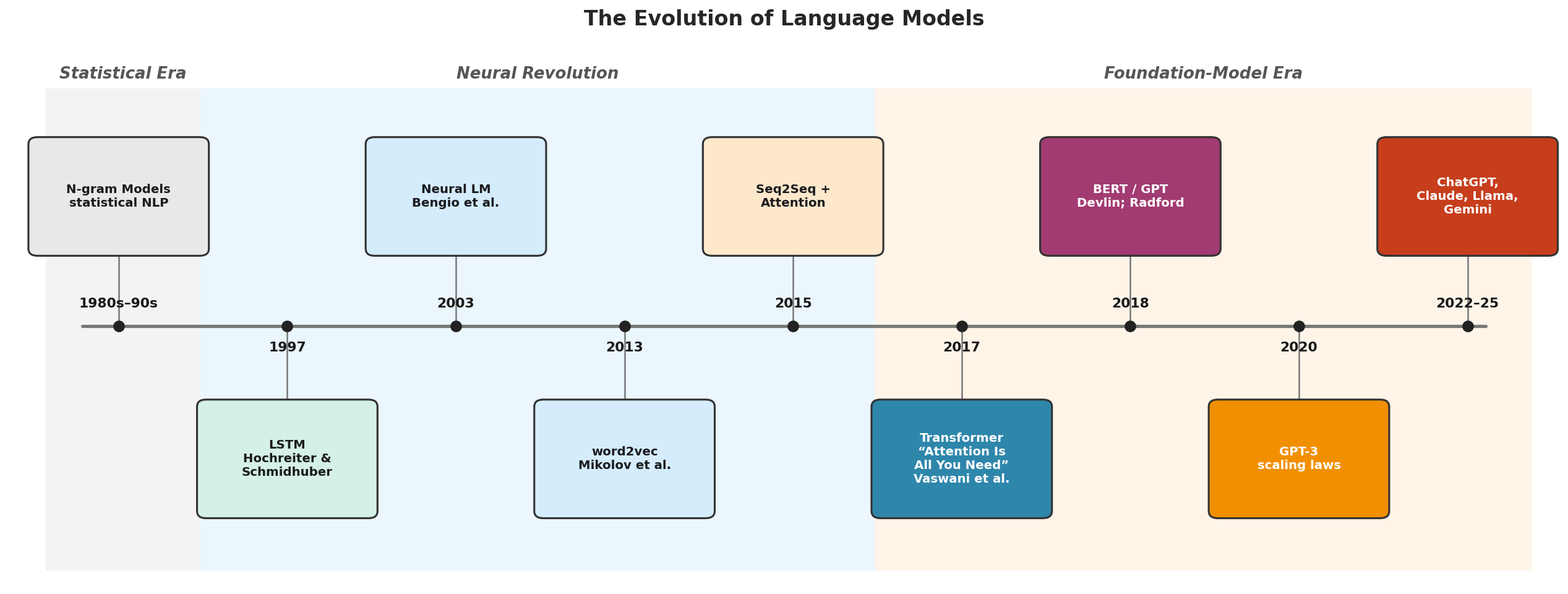
Timeline showing evolution of language models from n-gram models in the 1990s through Word2Vec, Transformers, BERT/GPT, and modern frontier models — Fig. 209 **Figure 6.1.1:** The evolution of language models. From statistical n-gram models in the 1990s through neural embeddings (Word2Vec, 2013), the transformer architecture (2017), and the foundation model era of GPT, Claude, Llama, and Gemini. Each transition brought qualitatively new capabilities.

Attention as Weighted Voting

The core idea of attention is intuitive: when processing a word in a sentence, the model should be able to “look at” all other words and decide which ones are relevant.

Consider the sentence: “The cat sat on the mat because it was tired.” To understand what “it” refers to, a model needs to connect “it” back to “cat”—which is six words earlier. An n-gram model with $n < 7$ cannot make this connection. An RNN might struggle because the information about “cat” has been compressed and potentially degraded as the hidden state passed through “sat,” “on,” “the,” and “mat.”

Attention solves this directly. When processing “it,” the model computes a relevance score between “it” and every other word in the sentence. These scores are normalized to form a probability distribution—the attention weights—and the output is a weighted combination of all words’ representations, with weights proportional to relevance.

Analogy: Attention as a Committee Vote

Attention also settles ambiguity. Take “I sat by the river bank.” Think of producing the representation for “bank” as a committee meeting in which every word votes on how relevant it is to “bank.” The word “river” votes strongly: “I’m highly relevant—I tell you which kind of bank this is!” Function words like “by” and “the” vote weakly, and “bank” keeps some of its own vote too.

The final representation of “bank” is a weighted combination of all words’ representations, with weights set by these votes—exactly the bar chart in the figure below. Because “river” wins the vote, “bank” ends up with the river/nature sense rather than the financial one. This is the essence of the self-attention mechanism.

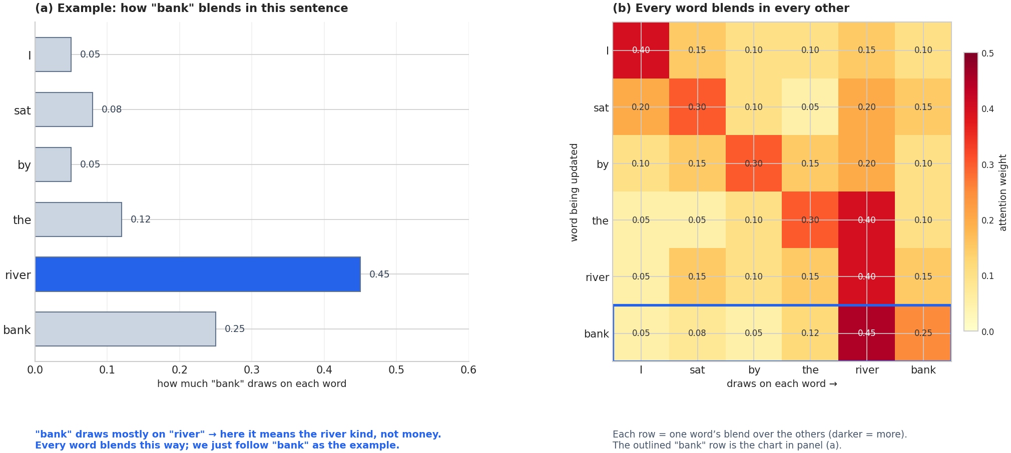
Two-panel attention figure — a bar chart of how much the word bank draws on each word in I sat by the river bank, and the full attention-weight heatmap for the sentence — Fig. 210 **Figure 6.1.2:** Attention as a weighted blend. (a) Following the word “bank” in *“I sat by the river bank,”* the model spreads its attention across the sentence and draws most heavily on “river”—so “bank” takes on the river/nature sense rather than the financial one. (b) The full attention-weight matrix for the sentence: each row shows how one word blends in all the others (darker = more attention; a probability distribution over the sentence), and the outlined “bank” row is the chart in panel (a).

Self-Attention, Multi-Head Attention, and Positional Encoding

The attention mechanism described above is called self-attention because a sequence attends to itself—each word looks at all other words in the same sequence. Formally, for each word, the model computes three vectors: a query (what am I looking for?), a key (what do I contain?), and a value (what information should I contribute?). The attention weight between two words is determined by the similarity between the query of one and the key of the other.

We present this conceptually rather than mathematically. What matters for data science practitioners is the consequence: attention allows the model to build context-dependent representations. The word “bank” gets a different representation in “river bank” versus “bank account” because it attends to different context words in each case.

Multi-head attention extends this by running multiple attention mechanisms in parallel, each with different learned parameters. Think of each “head” as looking for a different type of relationship: one head might focus on syntactic dependencies (subject-verb agreement), another on semantic relationships (synonym/antonym patterns), another on positional proximity. The outputs of all heads are concatenated and combined.

Positional encoding addresses a subtle problem: because attention operates on all words simultaneously (unlike RNNs, which process sequentially), the model has no inherent notion of word order. The sentence “dog bites man” and “man bites dog” would produce identical attention patterns without positional information. Positional encodings add information about each word’s position in the sequence, allowing the model to distinguish word order.

The Full Transformer Block

A single transformer block combines these components into a processing pipeline:

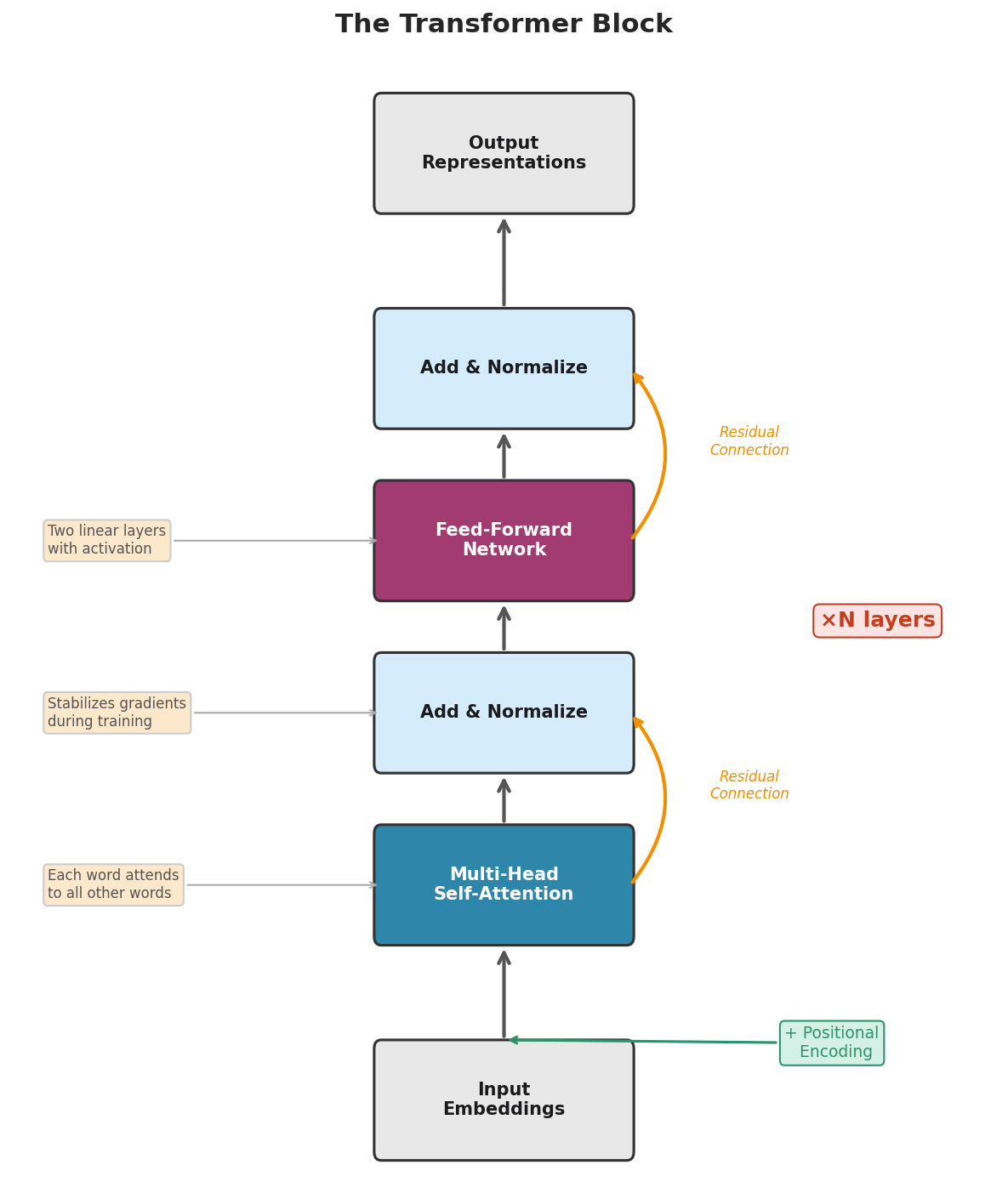
Annotated diagram of a transformer block showing multi-head attention, add and normalize, feed-forward network, and residual connections — Fig. 211 **Figure 6.1.3:** The transformer block. Input embeddings (with positional encoding) pass through multi-head self-attention, then through a feed-forward network. Each sub-layer has a residual connection (skip connection) and layer normalization. Real models stack N such blocks (N = 32 for a 7B model, N = 80+ for the largest models).

The key components are:

Multi-head self-attention: Each word attends to all others, producing context-aware representations.
Add & Normalize: The original input is added back (residual connection) and the result is normalized. Residual connections allow gradients to flow during training and help the model preserve information from earlier layers.
Feed-forward network: Two linear transformations with an activation function in between. This processes each position independently, adding nonlinear computational capacity.
Another Add & Normalize: Same residual + normalization pattern.

A complete transformer model stacks many such blocks. GPT-2 (2019) used 48 blocks. Llama 3.1 70B uses 80 blocks. Each block progressively refines the representations, building from surface-level patterns (spelling, syntax) in early layers to abstract concepts (sentiment, reasoning) in later layers.

Why This Matters for Data Scientists

You do not need to implement transformers. But understanding the architecture helps you:

Choose models wisely: Larger models (more layers, more parameters) capture more nuanced patterns but cost more to run.
Understand context windows: Attention computes pairwise interactions between all tokens, so computational cost grows quadratically with sequence length. This is why models have context window limits.
Interpret embeddings: The representations you extract in Section 6.2 come from specific layers of this architecture. Later layers capture more abstract features.
Debug failures: When a model fails to connect two pieces of information in a long document, the cause is often that they are too far apart for the attention mechanism to handle effectively.

Pre-Training, Fine-Tuning, and In-Context Learning

The capabilities of modern LLMs arise from three distinct phases, each contributing different kinds of knowledge and behavior.

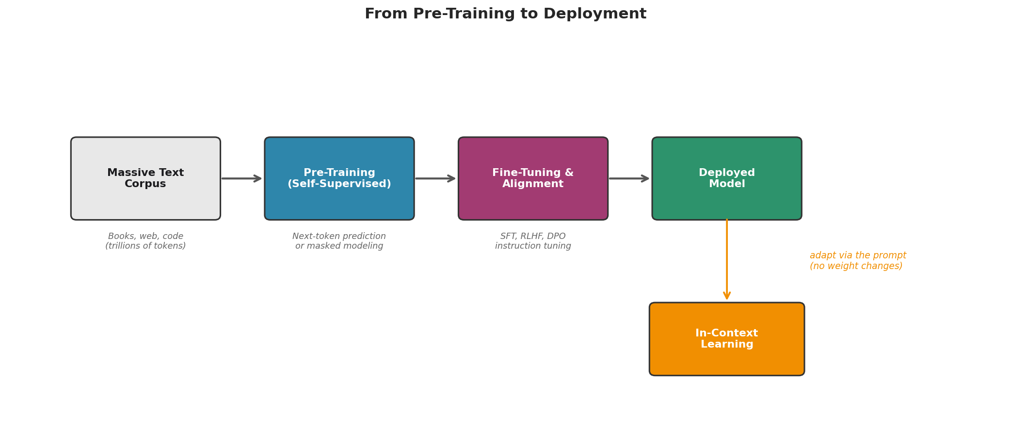
Pipeline diagram showing pre-training on massive corpus, fine-tuning with alignment, and deployment with in-context learning — Fig. 212 **Figure 6.1.4:** From pre-training to deployment. A massive text corpus is used for self-supervised pre-training (next-token prediction). The resulting base model is then fine-tuned with human feedback (RLHF) or preference optimization (DPO) to produce an aligned model ready for deployment. In-context learning allows further task-specific adaptation through the prompt alone, with no weight changes.

Pre-Training: Next Token Prediction and Masked Language Modeling

Pre-training is the phase that gives LLMs their broad knowledge and language capabilities. The idea is elegantly simple: train the model to predict what comes next.

Next-token prediction (used by GPT-family, Claude, Llama, Mistral): Given a sequence of words, predict the next word. The model sees “The capital of France is” and learns to predict “Paris.” Crucially, this single objective—applied to trillions of tokens from books, websites, code, scientific papers, and conversations—forces the model to learn an enormous amount about language, facts, reasoning, and even common sense.

Definition: Self-Supervised Learning

Self-supervised learning creates training labels from the data itself, without human annotation. In next-token prediction, each text naturally provides its own labels: every word is a “correct answer” for the preceding context. This eliminates the need for expensive human-labeled datasets and enables training on internet-scale corpora.

Masked language modeling (used by BERT-family models): Instead of predicting the next word, randomly mask 15% of words in a sentence and train the model to predict the masked words from context. Given “The [MASK] of France is Paris,” the model learns to predict “capital.” This produces models that are excellent at understanding text (classification, entity recognition) but not at generating text.

The distinction matters for data science applications:

Decoder-only models (GPT, Claude, Llama)—trained with next-token prediction—are strong at generation: writing text, completing prompts, following instructions.
Encoder-only models (BERT, RoBERTa)—trained with masked language modeling—are strong at understanding: classification, similarity, information extraction.
Encoder-decoder models (T5, BART)—trained with both—are strong at transformation: summarization, translation, reformulation.

For most data science tasks in this chapter, we use decoder-only models because they support the broadest range of capabilities through prompting.

Fine-Tuning and Alignment (RLHF, DPO)

A pre-trained model is a powerful but unrefined tool. It can complete any text plausibly, but it does not know to be helpful, to follow instructions, or to refuse harmful requests. It is equally happy completing a medical textbook or generating misinformation—it simply predicts the most likely next token given its training data.

Fine-tuning adapts a pre-trained model for specific behaviors. The most important form is instruction tuning, where the model is trained on examples of (instruction, desired response) pairs. After instruction tuning, the model understands that when a user asks a question, it should provide a helpful answer rather than simply continuing the text.

Reinforcement Learning from Human Feedback (RLHF) goes further. Human raters compare pairs of model responses and indicate which is better. These preferences are used to train a reward model, which then guides further training of the LLM. RLHF is what makes models like ChatGPT and Claude helpful, harmless, and honest—or at least, that is its aim.

Direct Preference Optimization (DPO) is a more recent alternative that achieves similar results without training a separate reward model. The model is trained directly on preference pairs, simplifying the pipeline while maintaining quality.

Key Insight: The Alignment Tax

Fine-tuning and alignment improve model behavior but can reduce raw capability. A base model might be better at completing obscure code patterns; an aligned model is better at following instructions safely. This trade-off—the “alignment tax”—is why some researchers work with base models for specific technical tasks. For data science workflows, aligned models are almost always preferable because they follow instructions reliably.

In-Context Learning: A Surprising Capability

Perhaps the most remarkable property of large language models is in-context learning: the ability to learn new tasks from examples provided in the prompt, without any change to the model’s parameters.

Consider this prompt:

Classify the sentiment of each review as positive or negative.

Review: “The food was excellent and the service was fast.” Sentiment: positive

Review: “Terrible experience. The room was dirty.” Sentiment: negative

Review: “Great location but the staff was rude.” Sentiment:

The model, having never been specifically trained on this particular sentiment classification task, can reliably complete this with “negative”—it has picked up both the label format and the judgment that rude staff outweighs a good location purely from the pattern of the examples. This is in-context learning—the model adapts its behavior based on the prompt context alone.

In-context learning is the foundation of prompt engineering (covered in depth in Section 6.6). It means we can customize model behavior for specific data science tasks without the cost and complexity of fine-tuning. We simply write better prompts.

Model Families and the Landscape

The LLM landscape as of 2026 is rich and evolving rapidly. Understanding the major model families helps you choose the right tool for each task.

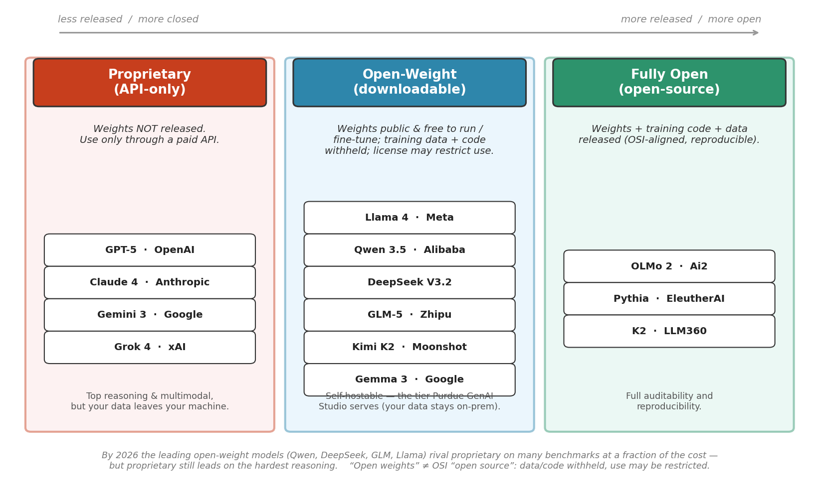
Scatter plot showing LLM families positioned by openness (open-weight vs proprietary) and relative capability — Fig. 213 **Figure 6.1.5:** The model landscape (2026), grouped by what the developer releases. *Proprietary / API-only* (GPT-5, Claude, Gemini, Grok): weights are never released. *Open-weight* (Llama 4, Qwen 3.5, DeepSeek, GLM-5, Kimi, Gemma): weights are downloadable and self-hostable, but the training data and code are withheld and the license may restrict use. *Fully open / OSI* (OLMo 2, Pythia, K2): weights, code, and data are released. By 2026 the leading open-weight models rival proprietary on many benchmarks at a fraction of the cost, though proprietary still leads on the hardest reasoning.

Proprietary Models: GPT, Claude, Gemini, Grok

GPT (OpenAI): The GPT family pioneered the large-scale decoder-only transformer. Its current flagship (the GPT-5 generation) is among the most capable general-purpose models, excelling at reasoning, code generation, and instruction following, while smaller mini variants provide a cost-effective option for simpler tasks.

Claude (Anthropic): The Claude family emphasizes safety and helpfulness through Constitutional AI—a training approach where the model critiques and revises its own outputs according to a set of principles. Claude models are known for careful, nuanced responses and strong performance on analytical tasks.

Gemini (Google DeepMind) and Grok (xAI): Multimodal proprietary families capable of processing text, images, audio, and video. Gemini is tightly integrated with Google’s ecosystem.

All of these models are available only through APIs: you send text to the provider’s servers and receive a response, which means your data leaves your premises—with implications for privacy and data governance that we take up in Section 6.9.

Open-Weight Models: Llama, Mistral, Gemma, DeepSeek

Llama (Meta): Meta’s open-weight family, now in its fourth generation with Llama 4, spans models from 1B to over 400B parameters. Llama 3.2 at 3B parameters runs on consumer hardware, the largest releases rival proprietary models, and the Llama 3.x generation remains widely deployed—including on GenAI Studio. The “open-weight” designation means the trained model weights are freely downloadable, but the training data and code may not be fully disclosed.

Mistral (Mistral AI): A French AI company producing efficient models. Mistral 7B punches above its weight class, performing comparably to much larger models on many benchmarks. The Mixtral series uses a Mixture-of-Experts architecture for efficiency.

Gemma (Google): Lightweight open-weight models derived from Gemini’s research. Gemma 3 at 12B parameters offers a good balance of capability and efficiency.

DeepSeek (DeepSeek AI): Chinese AI lab producing competitive open-weight models. DeepSeek-R1 is a large reasoning model trained to produce explicit chains of thought; its distilled variants bring that reasoning style to small models—the 1.5B–32B versions available on GenAI Studio.

Phi (Microsoft): Research-oriented small models designed to explore how much capability can be packed into a compact architecture. Phi-4 at 14B parameters is competitive with larger models on reasoning tasks.

Definition: Parameters and Model Size

A model’s parameter count (measured in billions, B) indicates the number of learnable weights in its neural network. Llama 3.2 at 3B has 3 billion parameters; GPT-4 is estimated at over 1 trillion. More parameters generally mean more capability but also more computational cost. A rough rule of thumb: a model requires approximately 2× its parameter count in bytes of memory in half-precision (FP16). So a 7B model needs ~14 GB of RAM/VRAM.

Scaling Laws and Emergent Abilities

Research by Kaplan et al. (2020) and Hoffmann et al. (2022, “Chinchilla”) revealed scaling laws: model performance improves predictably with increases in model size, training data, and compute. Specifically, loss decreases as a power law with each of these factors.

More intriguingly, some capabilities appear to emerge only above certain scale thresholds. Small models show little capacity for chain-of-thought reasoning or in-context learning; these abilities appear relatively suddenly as models grow past certain sizes—though distillation from a large reasoning model, as with DeepSeek-R1’s small variants, can transfer some of them back down. This phenomenon—called emergent abilities—remains actively debated: some researchers argue it reflects genuine phase transitions, while others attribute it to the choice of evaluation metrics.

For practitioners, the practical implication is: larger models can do qualitatively different things, not just quantitatively better things. A 3B model may classify sentiment competently but struggle with multi-step reasoning. A 70B model may handle both. Choosing the right model size for your task is a key practical decision.

A Moving Landscape: Where Frontier and Open-Weight Models Diverge

Figure 6.1.5 is a snapshot, and snapshots of this field age quickly. The specific names will change—some of the families in the figure will be superseded before this book is next revised—but the dynamics that generate the picture are far more stable, and they are what a data scientist should actually learn.

The most reliable dynamic of recent years is the catch-up cycle. A frontier lab demonstrates a new capability behind an API; within a year or two, open-weight releases reproduce most of it at a fraction of the size and cost. Distillation—training a smaller model to imitate the outputs of a stronger one—accelerates the cycle, and open releases by well-resourced labs (Meta’s Llama series, DeepSeek’s R1) periodically reset the baseline for everyone. Chain-of-thought reasoning followed exactly this path: introduced in proprietary frontier models, then distilled into open models small enough to run on the hardware behind GenAI Studio. The capability gap at any given moment is real, but it is perishable—plan on it narrowing for any capability that matters to routine data science work.

The catch-up cycle does not mean the two worlds converge to the same product, and it is worth being precise about vocabulary first. “Open-weight” means you can download the weights; it does not mean you get the training data, the training code, or an unrestricted license (Figure 6.1.5 separates these tiers deliberately). Weights without the recipe let you run, fine-tune, and audit the artifact, but not reproduce or fully interrogate its construction—and licenses vary enough that reading them is part of due diligence.

Where the families plausibly diverge going forward is along deployment structure, not a single quality scale. Frontier models are increasingly organized around what only massive, centrally served systems can offer: the longest-horizon reasoning and agentic workflows, frontier-scale multimodality, and tightly integrated tool-use ecosystems—capabilities you rent through an API and never hold. Open-weight models compete instead on what holding the model enables: on-premises privacy, fine-tuning for domain specialization, fixed cost at high volume, auditability, reproducibility through pinned weights, and deployment at the edge. These are different value propositions. A hospital system that must keep records in-house and a startup that needs one very hard reasoning call per day are not choosing between a better and a worse model; they are choosing between products built for different constraints.

Benchmark headlines are a poor guide to this choice, for three statistical reasons you are already equipped to see. Saturation: when top models cluster within a few points of a benchmark’s ceiling, leaderboard order is driven by noise—differences smaller than the evaluation’s standard error. Contamination: benchmark items leak into training corpora, so a score partly measures memorization rather than capability. Selection: developers announce the evaluations they win. Treat “Model X beats Model Y” the way Chapters 3 and 4 taught you to treat any comparison reported without uncertainty: as a claim, not a finding. What is worth tracking instead are the axes above—what open-weight models can now do on hardware you control, what frontier capability costs, what the license permits, and whether you can pin the exact model your results depend on.

The Practical Rule: Constraints First, Capability Second

Choose a model by deployment constraints first, capability second. Data governance (can the data leave your infrastructure?), cost structure (per-token or fixed?), and reproducibility (can you pin the exact weights your analysis depends on?) eliminate most options before capability ever enters the decision. This course’s own setup is an instance of the rule: Purdue GenAI Studio runs open-weight models on university hardware, so student data never leaves campus, the models behind your results stay pinned and reproducible, and the marginal cost of an API call is zero. Only when a task genuinely exceeds what an open-weight model can do—rare in routine data science—does frontier capability become the binding constraint.

Open vs. Closed Models: Trade-offs for Data Scientists

The choice between open-weight and proprietary models involves trade-offs along several dimensions:

Table 59 Open vs. Closed Model Trade-offs
Dimension	Open-Weight Models	Proprietary Models (API)
Privacy	Data stays on your infrastructure. No third-party access. Essential for sensitive data.	Data sent to provider’s servers. Subject to provider’s data policies. May not comply with institutional requirements.
Cost	Free to download and run. Cost is compute infrastructure (GPUs, electricity). Fixed cost regardless of usage volume.	Per-token pricing. Low barrier to start; costs scale with usage. No hardware investment needed.
Performance	Top open models (Llama 4, Qwen 3.5) approach proprietary performance. Smaller models (7–13B) are capable for focused tasks.	Generally highest capability, especially for complex reasoning. Regular updates without user effort.
Customization	Full fine-tuning possible. Can specialize for domain-specific tasks. Inspect and modify model behavior.	Limited to prompt engineering and API parameters. Some providers offer fine-tuning services.
Reproducibility	Same model version produces deterministic results (with fixed seed). Version control over model weights.	Provider may update models without notice. Same API call may produce different results over time.
Support	Community-driven. Quality varies. Requires ML engineering expertise.	Professional support. Managed infrastructure. Provider handles scaling.

For the data science workflows in this course, we use Purdue’s GenAI Studio, which provides the best of both worlds: open-weight models (Llama, Mistral, Gemma) running on institutional infrastructure, combining data privacy with ease of use.

Deployment Options

How you deploy an LLM determines your data privacy posture, cost structure, and available capabilities.

API-Based Services

Commercial APIs (OpenAI, Anthropic, Google) provide the simplest deployment path. You send a request, receive a response, and pay per token. No hardware management, no model configuration, no GPU procurement.

The trade-off is control. Your data traverses the internet and is processed on the provider’s infrastructure. While providers typically commit to not training on API inputs, the data is still temporarily present on their servers. For research involving human subjects data, HIPAA-protected information, or export-controlled material, this may be unacceptable.

Local Deployment with Ollama and Purdue GenAI Studio

Ollama is an open-source tool that makes it straightforward to run open-weight models locally. It handles model downloading, quantization, and serving with a simple command-line interface.

Purdue GenAI Studio takes this further by providing Ollama-backed models on Purdue’s Research Computing (RCAC) infrastructure. The key advantages:

Data privacy: All data stays on Purdue’s servers. Nothing leaves the institutional network.
No cost to students: Compute is provided by RCAC.
Multiple models: Access to Llama, Mistral, Gemma, DeepSeek, Phi, and others.
Familiar API: The genai_studio Python SDK provides an interface similar to the OpenAI SDK.

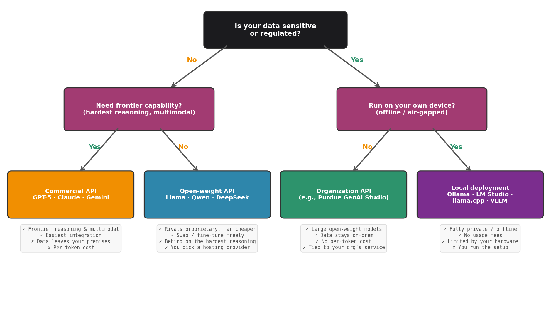
Decision tree for choosing between commercial API, open-weight, and local deployment based on data sensitivity and performance requirements — Fig. 214 **Figure 6.1.6:** Choosing a deployment strategy. The primary axis is data sensitivity. For non-sensitive data, choose a commercial API when you need frontier capability (hardest reasoning, multimodal), otherwise a cheaper open-weight API. For sensitive or regulated data, keep it in-house: an organization-hosted API such as Purdue’s GenAI Studio (large open-weight models on-premises, no per-token cost), or fully local deployment (Ollama, LM Studio, llama.cpp, vLLM) for an offline or air-gapped device.

Choosing a Deployment Strategy

For this course, the decision is straightforward: we use Purdue GenAI Studio for all exercises and projects. In professional practice, consider:

Start with the simplest option that meets your requirements. For most data science tasks, a capable open-weight model through GenAI Studio is sufficient.
Upgrade to commercial APIs when you need capabilities that open-weight models cannot match—complex multi-step reasoning, very long context windows, or multimodal processing.
Never send sensitive data to commercial APIs without explicit authorization from your data governance office.

Getting Started with GenAI Studio

The genai_studio SDK provides a clean Python interface to Purdue’s LLM infrastructure. Let us walk through the fundamentals.

Setting Up the Client

The first step is to create a client connection. You need an API key from GenAI Studio (Settings → Account → API Keys at https://genai.rcac.purdue.edu).

from genai_studio import GenAIStudio

ai = GenAIStudio()

print("Available models:")
for model in ai.models:
    print(f"  • {model}")

ai.select_model("gemma3:12b")
print(f"\nSelected model: {ai.model}")

Available models:
  • deepseek-r1:1.5b
  • gemma3:12b
  • llama3.2:latest
  • mistral:latest
  • phi4:latest
  ... (about 35 models in all)

Selected model: gemma3:12b

Note on Output Variability

LLM outputs are stochastic—the same prompt may produce different responses on different runs. Throughout this chapter, code outputs represent one plausible response. Your outputs will differ in wording but should convey the same content. This variability is a feature, not a bug, and we will study it formally in Section 6.8.

Your First Chat

The .chat() method sends a prompt and returns the response as a string:

response = ai.chat("What is the Central Limit Theorem? Answer in two sentences.")
print(response)

The Central Limit Theorem states that the sampling distribution of the
sample mean approaches a normal distribution as the sample size increases,
regardless of the population's original distribution. This fundamental
result underpins much of frequentist inference, enabling the construction
of confidence intervals and hypothesis tests even when the population
distribution is unknown.

Examining Response Metadata

The .chat_complete() method returns a rich response object that includes token counts—useful for understanding computational costs and context window usage:

response = ai.chat_complete(
    "Explain the difference between correlation and causation in one paragraph."
)

print(f"Response:\n{response.content}\n")
print(f"Model: {response.model}")
print(f"Finish reason: {response.finish_reason}")
print(f"Prompt tokens: {response.prompt_tokens}")
print(f"Completion tokens: {response.completion_tokens}")
print(f"Total tokens: {response.total_tokens}")

Response:
Correlation measures the statistical association between two variables—when
one changes, the other tends to change in a predictable way. Causation, on
the other hand, means that changes in one variable directly produce changes
in the other. The critical distinction is that correlation can arise from
confounding variables, reverse causation, or pure coincidence, whereas
causation requires a direct mechanism. The famous example: ice cream sales
and drowning deaths are correlated (both increase in summer), but ice cream
does not cause drowning—temperature is the confounding variable.

Model: gemma3:12b
Finish reason: stop
Prompt tokens: 18
Completion tokens: 112
Total tokens: 130

Streaming Responses

For longer responses, streaming displays tokens as they are generated rather than waiting for the complete response. This improves the user experience for interactive applications:

print("Streaming response:")
for chunk in ai.chat_stream("List three assumptions of linear regression."):
    print(chunk, end="", flush=True)
print()

Streaming response:
1. **Linearity**: The relationship between the independent variables and
the dependent variable is linear in the parameters.

2. **Independence of errors**: The residuals are independent of each
other, with no autocorrelation.

3. **Homoscedasticity**: The variance of the residuals is constant
across all levels of the independent variables.

Comparing Multiple Models

Different models have different strengths. Comparing responses helps you choose the right model for each task:

prompt = "What is a p-value? Explain simply in one sentence."
models = ["mistral:latest", "gemma3:12b", "llama3.2:latest"]

for model_name in models:
    ai.select_model(model_name)
    resp = ai.chat_complete(prompt)
    print(f"[{model_name}] ({resp.total_tokens} tokens)")
    print(f"  {resp.content}\n")

[mistral:latest] (67 tokens)
  A p-value is the probability of observing data as extreme as yours,
  assuming the null hypothesis is true.

[gemma3:12b] (82 tokens)
  A p-value represents the probability of obtaining test results at
  least as extreme as the observed results, under the assumption that
  the null hypothesis is correct.

[llama3.2:latest] (71 tokens)
  A p-value is the probability of seeing results as extreme as what
  you observed, if there were truly no effect or difference.

Using System Messages

System messages set the model’s behavior and persona for the entire conversation. They are distinct from user messages and are processed first:

ai.select_model("gemma3:12b")

system_msg = """You are a statistics professor at Purdue University.
You explain concepts precisely, using mathematical notation where
appropriate. Keep answers concise."""

response = ai.chat(
    "What is the difference between a parameter and a statistic?",
    system=system_msg
)
print(response)

A **parameter** is a fixed (but typically unknown) numerical characteristic
of a population, denoted with Greek letters: the population mean μ, the
population variance σ². A **statistic** is a function of sample data,
computed from observations: the sample mean x̄ = (1/n)Σxᵢ, the sample
variance s². Statistics are random variables (they vary from sample to
sample); parameters are constants. The goal of statistical inference is
to use statistics to learn about parameters.

Multi-Turn Conversations

The Conversation class manages multi-turn dialogue, automatically tracking message history:

from genai_studio import Conversation

conv = Conversation(system="You are a helpful data science tutor.")
conv.add_user("What is overfitting?")

response = ai.chat_conversation(conv)
print(f"Assistant: {response.content}\n")

conv.add_user("How does cross-validation help prevent it?")
response = ai.chat_conversation(conv)
print(f"Assistant: {response.content}")

Assistant: Overfitting occurs when a model learns the noise in the
training data rather than the underlying pattern. The model performs
excellently on training data but poorly on new, unseen data. It has
memorized rather than generalized.

Assistant: Cross-validation addresses overfitting by evaluating the
model on data it wasn't trained on. In k-fold cross-validation, the
data is split into k subsets. The model trains on k-1 folds and is
evaluated on the held-out fold, rotating through all folds. This gives
a more honest estimate of how the model will perform on new data,
exposing overfitting that would be hidden by training-set performance
alone.

Chapter 6.1 Exercises: LLM Foundations

A Note on These Exercises

These exercises introduce you to working with LLMs programmatically. Because LLM outputs are stochastic, your specific responses will differ from the solutions shown. Focus on the structure of the code and the approach to evaluation, not on matching outputs exactly.

Setup: All exercises assume you have configured genai_studio with a valid API key and can access at least two models (e.g., gemma3:12b and mistral:latest).

Exercise 6.1.1 — Model Comparison for Statistical Explanations

Use .chat_complete() to send the same statistical question to three different models. Compare response quality, token counts, and precision of statistical language.

(a) Define a list of 5 statistical concepts (e.g., “confidence interval,” “Bayes’ theorem,” “bootstrapping,” “maximum likelihood estimation,” “Markov chain”). For each concept, send the prompt "Define {concept} in exactly two sentences." to each of the three models.

(b) For each response, record: the model name, prompt tokens, completion tokens, and the response text. Display these in a structured table.

(c) Which model produces the most concise responses (fewest tokens)? Which produces the most technically precise responses (in your judgment)? Are these the same model?

Exercise 6.1.2 — System Message Engineering

System messages shape how the model responds. Explore this by using three different system messages to answer the same question.

(a) Write three system messages that instruct the model to respond as: (i) a statistics professor, (ii) a data journalist writing for a general audience, (iii) a cautious scientist who emphasizes uncertainty.

(b) Send the question "Is there evidence that class size affects student learning outcomes?" to the model with each system message. Record and display the three responses.

(c) Analyze how the system message changed: the vocabulary used, the level of hedging, the use of citations or evidence, and the overall tone. Write a brief paragraph summarizing your observations.

Exercise 6.1.3 — Token Counting and Cost Analysis

Understanding token usage is essential for managing computational costs and context windows.

(a) Create 5 prompts of increasing complexity: a single word, a simple question, a paragraph-length instruction, a detailed multi-part question, and a long prompt that includes a short dataset (formatted as text). Send each to the model using .chat_complete() and record prompt tokens and completion tokens.

(b) Plot prompt length (in words) versus prompt tokens. Is the relationship approximately linear? What is the approximate words-to-tokens ratio?

(c) Estimate the cost of processing 10,000 customer reviews (average 50 words each) for sentiment analysis, assuming a commercial API price of $0.15 per million input tokens and $0.60 per million output tokens. Assume each response is approximately 10 tokens.

Exercise 6.1.4 — Model Capabilities Inventory

Different models have different strengths. Create a systematic assessment.

(a) Design 4 test prompts, one for each capability category:

Factual recall: “What year was the Central Limit Theorem first formally stated, and by whom?”
Reasoning: “If a 95% confidence interval for μ is (3.2, 7.8), what is the point estimate and margin of error?”
Code generation: “Write a Python function that computes the bootstrap 95% confidence interval for the mean of a numpy array.”
Summarization: Provide a short paragraph of statistical text and ask for a one-sentence summary.

(b) Send each prompt to at least two models. For each response, rate accuracy on a 1-5 scale (you are the expert evaluator).

(c) Organize your results into a table: rows are test categories, columns are models, cells are your accuracy ratings. Which model performs best overall? Does any model dominate across all categories?

Transition to What Follows

With the foundations in place—architecture, training paradigms, model families, and the genai_studio SDK—we are ready to put LLMs to work. The next sections develop the core techniques for integrating LLMs into data science workflows.

Section 6.2 introduces embeddings: dense vector representations of text that capture semantic meaning. You will learn to generate embeddings, use them for similarity search, decode what each dimension encodes, and integrate embedding-derived features into the statistical models from Chapters 3 and 4. Embeddings transform unstructured text into the kind of numerical data that your statistical toolkit can process.

Following that, Section 6.3 develops the text preprocessing pipeline—tokenization, chunking, and normalization—that prepares documents for LLM consumption. These techniques become critical when building retrieval-augmented generation systems in Section 6.5.

The thread connecting all subsequent sections is this: LLMs are powerful but imperfect tools. Using them effectively requires the same rigor we have applied throughout this course—careful problem formulation, appropriate methods, honest evaluation, and transparent reporting of limitations.

Key Takeaways 📝

Transformer architecture: The attention mechanism allows each word to attend to all other words, enabling context-dependent representations. Multi-head attention captures different types of relationships in parallel. This architecture eliminated the sequential processing bottleneck of RNNs and enabled training on massive datasets.
Three phases of capability: Pre-training (self-supervised learning on trillions of tokens) provides broad knowledge. Fine-tuning and alignment (RLHF, DPO) shape model behavior to be helpful and safe. In-context learning (prompt-based adaptation) enables task-specific customization without changing model weights.
Model landscape: Proprietary models (GPT, Claude, Gemini) offer the highest capability via API but raise privacy concerns. Open-weight models (Llama, Mistral, Gemma) can be run locally with full data control. The capability gap between open and closed models has narrowed substantially.
Deployment choice: For this course, Purdue GenAI Studio provides open-weight models on institutional infrastructure—combining data privacy, zero cost, and a clean Python API via the genai_studio SDK.
Practical awareness: LLM outputs are stochastic (same prompt, different responses), have context window limits (attention cost grows quadratically), and reflect their training data (including biases and knowledge cutoffs). These characteristics shape how we use and evaluate LLMs in subsequent sections.