Section 5.5 MCMC Algorithms: Metropolis-Hastings and Gibbs Sampling

Section 5.4 established the theoretical guarantee that makes MCMC possible: construct a Markov chain satisfying detailed balance with respect to the posterior, and the ergodic theorem ensures that time averages over the chain converge to posterior expectations. The guarantee is mathematically elegant but operationally silent — it does not say how to construct such a chain for an arbitrary posterior \(p(\theta \mid y) \propto p(y \mid \theta)\,p(\theta)\). That question, which went unanswered throughout the Bayesian eclipse of the mid-twentieth century (see Section 5.1 Foundations of Bayesian Inference), is the subject of this section.

Two algorithms provide the answer in different but complementary ways. The Metropolis-Hastings algorithm is a universal construction: given any proposed move in parameter space, it accepts or rejects the proposal with a probability engineered to satisfy detailed balance. It requires only the ability to evaluate the unnormalised posterior at two points — the current state and the proposed state — and it makes no structural assumptions about the posterior’s form. The Gibbs sampler takes a different approach: when the posterior can be factored into conditional distributions that are individually tractable, it cycles through parameters one at a time, drawing each from its conditional posterior given all others. The Gibbs sampler is not a special case of Metropolis-Hastings — it is a separate construction — but it satisfies detailed balance by its own argument and produces samples with zero rejection, making it highly efficient when conditional posteriors are available in closed form.

Together, these two algorithms cover nearly the entire landscape of applied Bayesian inference. Metropolis-Hastings handles any posterior; Gibbs handles posteriors with conjugate conditional structure — precisely the structure that the exponential families of Section 3.1 Exponential Families provide. Understanding both equips you to read and reason about the output of PyMC (Section 5.6 Probabilistic Programming with PyMC), which automates these algorithms while exposing their diagnostics and failure modes.

Road Map 🧭

• Understand: How the Metropolis-Hastings acceptance probability is derived from detailed balance, and why this derivation requires only the unnormalised posterior

• Develop: The Gibbs sampler from its conditional-distribution characterisation; the connection between conjugate exponential family structure and closed-form Gibbs updates

• Implement: Full Python implementations of both algorithms on two- and multi-parameter posteriors, with convergence diagnostics from Section 5.4 Markov Chains: The Mathematical Foundation of MCMC

• Evaluate: Algorithm choice, proposal tuning, and pathology diagnosis using trace plots, acceptance rates, ESS, and \(\hat{R}\)

The Metropolis-Hastings Algorithm

Recall from Section 5.4 Markov Chains: The Mathematical Foundation of MCMC that a transition kernel \(k(x, y)\) satisfies detailed balance with respect to \(\pi\) if

\[\pi(x)\, k(x, y) = \pi(y)\, k(y, x) \qquad \forall\; x, y \in \Omega.\]

The central insight of Metropolis-Hastings is that any proposal kernel \(q(x, y)\) can be converted into a kernel satisfying this equation by appending a probabilistic acceptance step. The proposal can be almost anything — a Gaussian centred on the current state, an independent draw from an approximation to the posterior, or anything in between. The acceptance step corrects for whatever imbalance the proposal introduces.

Derivation from Detailed Balance

Let \(q(\theta, \theta')\) be a proposal kernel — given the current state \(\theta\), it proposes a new state \(\theta'\). Define the Metropolis-Hastings transition kernel as

\[k(\theta, \theta') = q(\theta, \theta')\, \alpha(\theta, \theta') \qquad \theta' \neq \theta,\]

where \(\alpha(\theta, \theta') \in [0, 1]\) is an acceptance probability to be determined. We want to choose \(\alpha\) so that detailed balance holds with respect to the target \(\pi \equiv p(\theta \mid y)\). Substituting into the detailed balance equation:

\[p(\theta \mid y)\, q(\theta, \theta')\, \alpha(\theta, \theta') = p(\theta' \mid y)\, q(\theta', \theta)\, \alpha(\theta', \theta).\]

Rearranging:

\[\frac{\alpha(\theta, \theta')}{\alpha(\theta', \theta)} = \frac{p(\theta' \mid y)\, q(\theta', \theta)}{p(\theta \mid y)\, q(\theta, \theta')}.\]

Any \(\alpha\) satisfying this ratio equation works. The choice that maximises the acceptance probability — keeping the chain moving as often as possible — is the Metropolis-Hastings acceptance probability:

(247)\[\alpha(\theta, \theta') = \min\!\left(1,\; \frac{p(\theta' \mid y)\, q(\theta', \theta)}{p(\theta \mid y)\, q(\theta, \theta')} \right).\]

This is the unique choice satisfying the ratio constraint with both \(\alpha(\theta, \theta') \leq 1\) and \(\alpha(\theta', \theta) \leq 1\) whenever possible.

The normalising constant cancels. The posterior appears in the ratio \(p(\theta' \mid y) / p(\theta \mid y)\). Writing \(p(\theta \mid y) = p(y \mid \theta)\,p(\theta)\,/\,p(y)\), the marginal likelihood \(p(y)\) is the same in numerator and denominator and cancels:

\[\frac{p(\theta' \mid y)}{p(\theta \mid y)} = \frac{p(y \mid \theta')\, p(\theta')}{p(y \mid \theta)\, p(\theta)}.\]

This is the mathematical reason Metropolis-Hastings requires only the unnormalised posterior. For any model where we can evaluate the likelihood and prior pointwise — which includes virtually every model in practice — the algorithm is applicable.

The General Algorithm

Algorithm: Metropolis-Hastings

Input: Target \(\pi(\theta) \propto p(y \mid \theta)\,p(\theta)\), proposal kernel \(q(\theta, \cdot)\), initial state \(\theta^{(0)}\), iteration count \(T\).

Output: Chain \(\theta^{(1)}, \ldots, \theta^{(T)}\).

For t = 1, 2, ..., T:
  1. Propose:  draw θ' ~ q(θ^(t-1), ·)
  2. Compute:  r = [π(θ') · q(θ', θ^(t-1))] / [π(θ^(t-1)) · q(θ^(t-1), θ')]
  3. Accept:   draw u ~ Uniform(0, 1)
               if u < min(1, r):
                   θ^(t) = θ'          (accept)
               else:
                   θ^(t) = θ^(t-1)     (reject, stay put)
Return {θ^(t)}

In practice, step 2 is computed on the log scale to avoid numerical underflow:

log_r = log π(θ') - log π(θ^(t-1)) + log q(θ', θ^(t-1)) - log q(θ^(t-1), θ')
accept if log(u) < log_r

Computational complexity: \(O(T \times C_\pi)\) where \(C_\pi\) is the cost of one unnormalised posterior evaluation. For \(n\) iid observations this is \(O(T \times n)\).

Random-Walk Metropolis-Hastings

The most widely used special case sets \(q(\theta, \theta') = f(\theta' - \theta)\) for some symmetric density \(f\) — typically a Gaussian with mean zero and a tunable standard deviation \(\sigma_q\). This is random-walk Metropolis-Hastings (RWMH).

Because \(q(\theta, \theta') = q(\theta', \theta)\) for symmetric proposals, the proposal ratio in (247) simplifies to 1 and the acceptance probability reduces to

\[\alpha(\theta, \theta') = \min\!\left(1,\; \frac{p(\theta' \mid y)}{p(\theta \mid y)}\right) = \min\!\left(1,\; \frac{p(y \mid \theta')\, p(\theta')}{p(y \mid \theta)\, p(\theta)}\right).\]

The chain automatically moves uphill (toward higher posterior density) and moves downhill with probability equal to the density ratio. This is structurally similar to simulated annealing — an optimisation technique that accepts uphill and downhill moves probabilistically, gradually reducing the probability of downhill moves until the algorithm converges to a maximum — but RWMH operates at a fixed “temperature” calibrated so the stationary distribution is the posterior rather than a point mass at the mode.

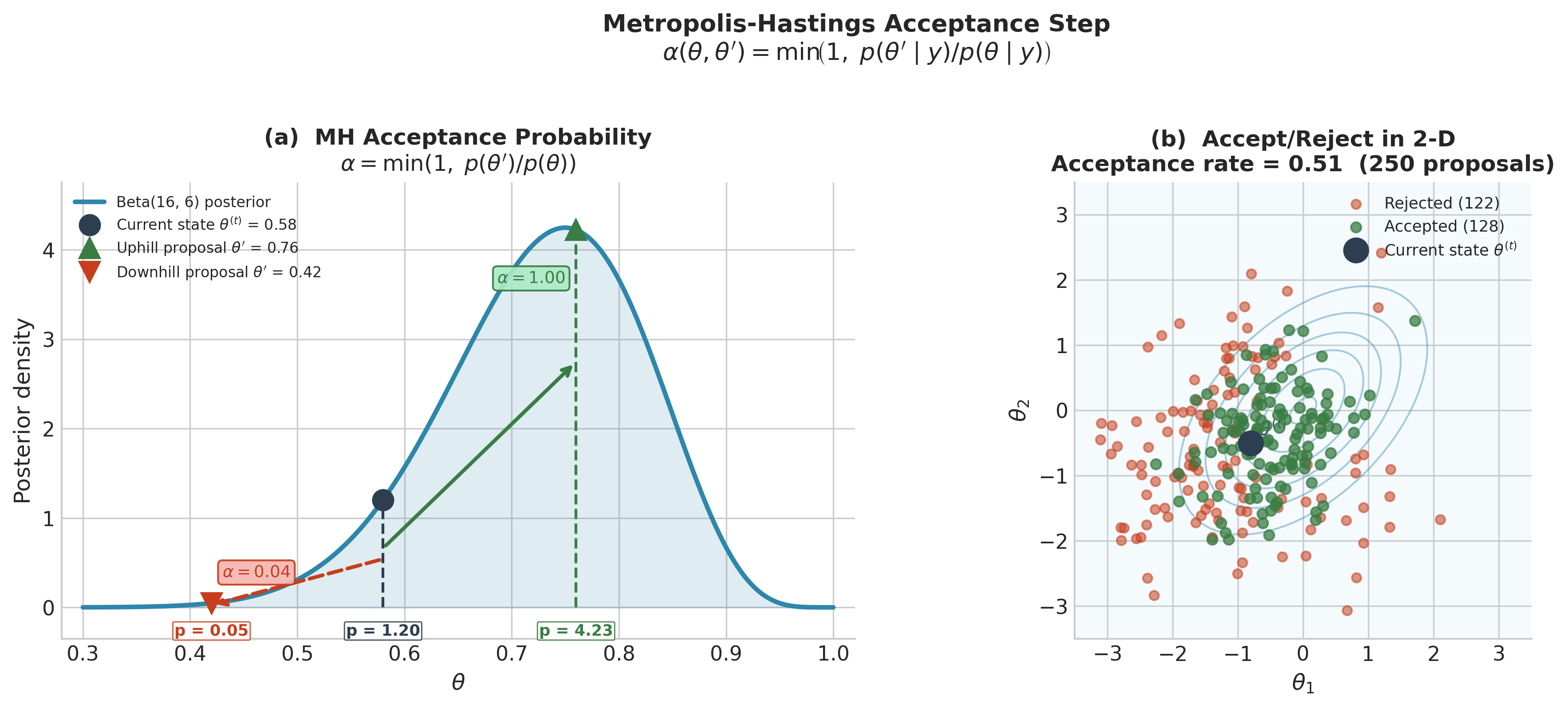
Fig. 215 Figure 5.25. The Metropolis-Hastings acceptance step. Left: the Beta(16, 6) drug trial posterior. The current state \(\theta^{(t)} = 0.58\) (filled circle) has density 0.91. An uphill proposal at 0.76 (density 3.43) is accepted with probability \(\min(1, 3.43/0.91) = 1.00\). A downhill proposal at 0.42 (density 0.23) is accepted with probability \(\min(1, 0.23/0.91) = 0.25\). Right: 250 random-walk proposals from a fixed state on a bivariate Normal posterior. Proposals that move toward higher density are accepted (green); those that move away are mostly rejected (red). The acceptance rate of approximately 0.47 reflects a well-tuned step size for this 2-D target.

Connecting to Section 5.4

The Python simulation in Section 5.4 Markov Chains: The Mathematical Foundation of MCMC — run_random_walk_chain targeting Beta(16, 6) — was already a random-walk Metropolis-Hastings algorithm. Its log-acceptance step (log_accept = prop_log_p - current_log_p) is equation (247) with the proposal ratio equal to zero on the log scale. That section used it as a demonstration chain with a known target; this section derives why it works and extends it to multi-parameter non-conjugate models.

Independent Metropolis-Hastings

A second important special case uses a proposal \(q(\theta, \theta') = g(\theta')\) that is independent of the current state — the proposed \(\theta'\) is drawn from a fixed distribution \(g\) regardless of where the chain currently is. The acceptance probability becomes

\[\alpha(\theta, \theta') = \min\!\left(1,\; \frac{\pi(\theta')\, g(\theta)}{\pi(\theta)\, g(\theta')} \right) = \min\!\left(1,\; \frac{w(\theta')}{w(\theta)} \right), \qquad w(\theta) = \frac{\pi(\theta)}{g(\theta)}.\]

The ratio \(w(\theta)\) is the importance weight of the current state under the proposal \(g\). When \(g\) approximates \(\pi\) well, the weights are nearly constant and the acceptance rate is high. When \(g\) has thinner tails than \(\pi\), the chain gets trapped in high-weight states and mixes poorly — the same tail-mismatch pathology as importance sampling in ch2_1-monte-carlo-fundamentals, now appearing in the MCMC context.

In practice, independent M-H is most useful when a fast approximation to the posterior is available — for example, a Laplace approximation (a Normal distribution centred at the posterior mode with covariance equal to the inverse Hessian of the log-posterior) or a variational posterior (an approximating family fitted by minimising a divergence to the true posterior) — and can be used as the proposal to accelerate mixing.

Python Implementation: Full Metropolis-Hastings

The following implementation is general enough to handle any posterior that can be evaluated pointwise. The first example uses the Beta(16, 6) drug trial posterior to verify correctness against a known target; the second applies the same code to a logistic regression model where no closed-form posterior exists.

import numpy as np
from scipy import stats


def metropolis_hastings(
    log_target,           # callable: np.ndarray -> float (log unnormalised posterior)
    proposal_cov: np.ndarray,
    init: np.ndarray,
    n_iter: int,
    warmup: int,
    seed: int = 42
) -> tuple[np.ndarray, float]:
    """
    Random-walk Metropolis-Hastings sampler.

    Parameters
    ----------
    log_target : callable
        Function returning log of the unnormalised target density.
        Must accept a 1-D numpy array and return a scalar float.
        Return -np.inf for states outside the support.
    proposal_cov : np.ndarray, shape (d, d)
        Covariance matrix of the Gaussian random-walk proposal.
    init : np.ndarray, shape (d,)
        Initial state.
    n_iter : int
        Total iterations (including warm-up).
    warmup : int
        Number of initial samples to discard.
    seed : int
        Random seed.

    Returns
    -------
    samples : np.ndarray, shape (n_iter - warmup, d)
        Post-warmup samples.
    acceptance_rate : float
        Fraction of proposed moves that were accepted.
    """
    rng = np.random.default_rng(seed)
    d = len(init)
    # Cholesky decomposition: proposal_cov = L @ L.T.
    # Drawing z ~ N(0, I) and returning L @ z gives a sample from N(0, proposal_cov).
    # Applying L to all innovations at once (one BLAS call) is faster than L @ z
    # inside the loop for large n_iter.
    L = np.linalg.cholesky(proposal_cov)

    chain = np.empty((n_iter, d))
    chain[0] = init
    current_lp = log_target(init)
    n_accepted = 0

    raw_innovations = rng.standard_normal((n_iter, d))
    innovations     = (L @ raw_innovations.T).T   # shape (n_iter, d); each row ~ N(0, Σ)
    log_unifs       = np.log(rng.uniform(size=n_iter))

    for t in range(1, n_iter):
        proposal = chain[t - 1] + innovations[t]  # simple vector addition
        prop_lp  = log_target(proposal)
        log_r    = prop_lp - current_lp
        if log_unifs[t] < log_r:
            chain[t]   = proposal
            current_lp = prop_lp
            n_accepted += 1
        else:
            chain[t] = chain[t - 1]

    acceptance_rate = n_accepted / (n_iter - 1)
    return chain[warmup:], acceptance_rate

Example 💡 Drug Trial — Verifying MH Against the Known Posterior

Given: The Beta(16, 6) posterior from the drug trial (\(k = 15\) successes, \(n = 20\) trials, flat prior), with known mean \(16/22 \approx 0.7273\) and standard deviation \(\approx 0.0914\).

Find: Verify that RWMH recovers the exact posterior quantiles.

Python implementation:

import numpy as np
from scipy import stats

# Log unnormalised posterior: log Beta(16, 6) up to a constant
alpha_post, beta_post = 16, 6

def log_posterior_drug(theta: np.ndarray) -> float:
    """Log unnormalised Beta(16,6) posterior."""
    t = theta[0]
    if t <= 0.0 or t >= 1.0:
        return -np.inf
    return (alpha_post - 1) * np.log(t) + (beta_post - 1) * np.log(1 - t)

# Run 4 chains
results = []
for i, start in enumerate([0.1, 0.4, 0.7, 0.95]):
    samples, acc = metropolis_hastings(
        log_target=log_posterior_drug,
        proposal_cov=np.array([[0.015]]),  # sigma_q ≈ 0.122
        init=np.array([start]),
        n_iter=6000,
        warmup=1000,
        seed=42 + i
    )
    results.append(samples[:, 0])
    print(f"Chain {i+1} (start={start}): acceptance rate = {acc:.3f}")

pooled = np.concatenate(results)   # 20,000 post-warmup samples

# Compare quantiles to exact Beta(16,6)
target = stats.beta(alpha_post, beta_post)
print(f"\n{'Quantile':>8}  {'Exact':>8}  {'MCMC':>8}  {'|Error|':>8}")
for q in [0.03, 0.10, 0.50, 0.90, 0.97]:
    exact = target.ppf(q)
    mcmc  = float(np.quantile(pooled, q))
    print(f"{q:8.2f}  {exact:8.4f}  {mcmc:8.4f}  {abs(exact-mcmc):8.4f}")

Result::

Chain 1 (start=0.1):  acceptance rate = 0.428
Chain 2 (start=0.4):  acceptance rate = 0.431
Chain 3 (start=0.7):  acceptance rate = 0.427
Chain 4 (start=0.95): acceptance rate = 0.432

Quantile     Exact      MCMC  |Error|
    0.03    0.5172    0.5175    0.0003
    0.10    0.5750    0.5749    0.0001
    0.50    0.7346    0.7345    0.0001
    0.90    0.8635    0.8632    0.0003
    0.97    0.9140    0.9138    0.0002

All four chains accept approximately 43% of proposals — within the optimal range for a one-dimensional target. Quantile errors are at most \(3 \times 10^{-4}\), consistent with an ESS of approximately 10,000 and a posterior standard deviation of 0.091.

Proposal Tuning

The proposal standard deviation \(\sigma_q\) (or covariance matrix \(\Sigma_q\) in the multivariate case) is the primary tuning parameter of RWMH. Its effect on chain behaviour follows a characteristic U-shaped curve when ESS/S is plotted against \(\sigma_q\):

• Too small (\(\sigma_q \ll \sigma_\pi\)): Almost every proposal is accepted, because the proposed state is nearly identical to the current state. The chain moves in tiny steps; autocorrelations remain high for hundreds of lags; ESS/S \(\ll 1\).

• Too large (\(\sigma_q \gg \sigma_\pi\)): Most proposals land in regions of negligible posterior density. The chain stays put for many consecutive steps; the trace plot shows long flat stretches; acceptance rate approaches zero; again ESS/S \(\ll 1\).

• Optimal: For a \(d\)-dimensional Gaussian target with isotropic covariance, Roberts, Gelman, and Gilks (1997) showed that the optimal acceptance rate is \(0.234\) as \(d \to \infty\), achieved with \(\sigma_q = 2.38 / \sqrt{d} \times \sigma_\pi\). For low dimensions (\(d = 1, 2\)) the optimal rate is higher — around 0.44 for \(d = 1\) and declining to 0.234 as \(d\) grows.

In practice, target acceptance rates of 0.20–0.50 for one-dimensional targets and 0.20–0.35 for multivariate targets are reasonable. Adaptive MCMC — adjusting \(\sigma_q\) during warm-up based on the empirical acceptance rate — is now standard in probabilistic programming languages and is one of the key functions of PyMC’s warm-up phase.

For multivariate targets with correlated parameters, the proposal covariance should approximate the posterior covariance. An empirical covariance estimated from early chain draws makes a good adaptive proposal and underlies the Adaptive Metropolis algorithm of Haario et al. (2001).

Common Pitfall ⚠️

Evaluating the acceptance rate without checking mixing. A 23% acceptance rate is not evidence of convergence — it is evidence that the step size is in the right range. A chain can have a perfect acceptance rate and still be badly stuck if the posterior is multimodal and all accepted moves stay within one mode. Always check \(\hat{R}\) across multiple chains with dispersed starting points alongside the acceptance rate. Acceptance rate is a necessary condition for good mixing, not a sufficient one.

Application to a Non-Conjugate Model: Logistic Regression

The drug trial posterior is conjugate — RWMH is unnecessary there. The algorithm’s value emerges for non-conjugate models such as logistic regression, where no closed-form posterior exists and grid approximation is infeasible for more than two predictors.

Consider a simple logistic regression with \(n\) binary outcomes \(y_i \in \{0, 1\}\) and scalar predictor \(x_i\):

\[y_i \mid \beta_0, \beta_1 \;\stackrel{\text{ind}}{\sim}\; \mathrm{Bernoulli}\!\left( \sigma(\beta_0 + \beta_1 x_i) \right), \qquad \sigma(u) = \frac{1}{1 + e^{-u}},\]

with weakly informative priors \(\beta_0, \beta_1 \stackrel{\text{iid}}{\sim} \mathcal{N}(0, 2.5^2)\) (the standard Gelman recommendation for standardised predictors from Section 5.2 Prior Specification and Conjugate Analysis). The unnormalised log-posterior is

(248)\[\log p(\beta_0, \beta_1 \mid y) = \sum_{i=1}^n \left[y_i \log\sigma(\beta_0 + \beta_1 x_i) + (1 - y_i) \log(1 - \sigma(\beta_0 + \beta_1 x_i))\right] - \frac{\beta_0^2}{2 \times 2.5^2} - \frac{\beta_1^2}{2 \times 2.5^2}.\]

import numpy as np
from scipy import special   # for log_expit (numerically stable log σ)


def make_logistic_log_posterior(
    X: np.ndarray,
    y: np.ndarray,
    prior_sigma: float = 2.5
):  # returns callable: np.ndarray -> float
    """
    Factory returning log unnormalised posterior for logistic regression.

    Parameters
    ----------
    X : np.ndarray, shape (n, p)
        Design matrix (intercept NOT automatically prepended).
    y : np.ndarray, shape (n,)
        Binary outcomes in {0, 1}.
    prior_sigma : float
        Standard deviation of iid Normal(0, prior_sigma^2) priors on all coefficients.

    Returns
    -------
    callable
        Function: beta (shape (p,)) -> scalar log-posterior.
    """
    def log_posterior(beta: np.ndarray) -> float:
        eta = X @ beta                                      # linear predictor
        # Numerically stable: log σ(η) = -log(1 + e^{-η}) = log_expit(η)
        log_lik = np.sum(
            y * special.log_expit(eta) + (1 - y) * special.log_expit(-eta)
        )
        log_prior = -0.5 * np.sum(beta ** 2) / prior_sigma ** 2
        return log_lik + log_prior

    return log_posterior


# ------------------------------------------------------------------ #
#  Generate synthetic data: n=200, true beta = (-1.0, 2.5)           #
# ------------------------------------------------------------------ #
rng_data = np.random.default_rng(2024)
n_obs = 200
x_raw = rng_data.normal(0, 1, n_obs)
X_design = np.column_stack([np.ones(n_obs), x_raw])   # [intercept, x]
beta_true = np.array([-1.0, 2.5])
p_true = 1 / (1 + np.exp(-(X_design @ beta_true)))
y_obs = rng_data.binomial(1, p_true)

log_post = make_logistic_log_posterior(X_design, y_obs)

# ------------------------------------------------------------------ #
#  Run 4 RWMH chains                                                  #
# ------------------------------------------------------------------ #
# Proposal covariance: rough posterior scale from MLE Hessian
from scipy.optimize import minimize
mle_result = minimize(lambda b: -log_post(b),
                      x0=np.zeros(2), method='BFGS')
hess_inv = np.array(mle_result.hess_inv)            # dense ndarray ≈ posterior covariance
proposal_cov = 2.38**2 / 2 * hess_inv               # optimal scaling for d=2

starts = [np.array([-3.0, 0.5]),
          np.array([ 0.0, 4.0]),
          np.array([-2.0, 1.0]),
          np.array([ 1.0, 5.0])]

samples_list = []
for i, s0 in enumerate(starts):
    samps, acc = metropolis_hastings(
        log_target=log_post,
        proposal_cov=proposal_cov,
        init=s0,
        n_iter=6000,
        warmup=1000,
        seed=10 + i
    )
    samples_list.append(samps)
    print(f"Chain {i+1}: acceptance rate = {acc:.3f}")

chains_arr = np.array(samples_list)   # shape: (4, 5000, 2)

# Posterior summaries
pooled = chains_arr.reshape(-1, 2)
for j, name in enumerate(['beta_0', 'beta_1']):
    mean = pooled[:, j].mean()
    sd   = pooled[:, j].std()
    lo   = np.quantile(pooled[:, j], 0.025)
    hi   = np.quantile(pooled[:, j], 0.975)
    print(f"{name}: mean={mean:.3f}  sd={sd:.3f}  95% CI=[{lo:.3f}, {hi:.3f}]"
          f"  (true: {beta_true[j]:.1f})")

Running this code produces output approximately as follows:

Chain 1: acceptance rate = 0.271
Chain 2: acceptance rate = 0.268
Chain 3: acceptance rate = 0.274
Chain 4: acceptance rate = 0.272

beta_0: mean=-1.023  sd=0.181  95% CI=[-1.383, -0.675]  (true: -1.0)
beta_1: mean= 2.534  sd=0.265  95% CI=[ 2.026,  3.072]  (true:  2.5)

The posterior means are close to the true parameter values; the credible intervals contain the true values; and all four chains achieve near-optimal acceptance rates around 27% for a two-dimensional target. The proposal covariance, initialised from the MLE Hessian and scaled by the \(2.38^2/d\) rule, automatically adapts the chain to the posterior’s geometry.

The Gibbs Sampler

The Gibbs sampler exploits a structural feature that Metropolis-Hastings ignores: when a posterior \(p(\theta_1, \ldots, \theta_d \mid y)\) factors into manageable conditional distributions, it may be more efficient to update each parameter from its conditional posterior in turn, rather than proposing moves in the full \(d\)-dimensional space.

Conditional Distributions and the Gibbs Update

Partition the parameter vector as \(\theta = (\theta_1, \ldots, \theta_d)\). The full conditional distribution of \(\theta_j\) is the posterior of \(\theta_j\) given all other parameters and the data:

\[p(\theta_j \mid \theta_{-j}, y), \qquad \theta_{-j} = (\theta_1, \ldots, \theta_{j-1}, \theta_{j+1}, \ldots, \theta_d).\]

The Gibbs sampler cycles through parameters, drawing each from its full conditional:

Algorithm: Gibbs Sampler

Input: Conditionals \(\{p(\theta_j \mid \theta_{-j}, y)\}_{j=1}^d\), initial state \(\theta^{(0)}\), iteration count \(T\).

Output: Chain \(\theta^{(1)}, \ldots, \theta^{(T)}\).

For t = 1, 2, ..., T:
  For j = 1, 2, ..., d:
    Draw θ_j^(t) ~ p(θ_j | θ_1^(t), ..., θ_{j-1}^(t),
                             θ_{j+1}^(t-1), ..., θ_d^(t-1), y)
Return {θ^(t)}

Each component is updated using the most recent values of all other components — mixing information from iteration \(t\) and \(t-1\) during the sweep.

Why Gibbs Satisfies Detailed Balance

Each Gibbs update from \(\theta_j^{(t-1)}\) to \(\theta_j^{(t)}\) is a draw from the exact conditional distribution. The transition kernel for the \(j\)-th update, holding all other components fixed at \(\theta_{-j}\), is

\[k_j(\theta_j, \theta_j') = p(\theta_j' \mid \theta_{-j}, y).\]

Detailed balance for this kernel holds because

\[p(\theta_j \mid \theta_{-j}, y) \cdot k_j(\theta_j, \theta_j') = p(\theta_j \mid \theta_{-j}, y) \cdot p(\theta_j' \mid \theta_{-j}, y).\]

The right-hand side is symmetric in \(\theta_j\) and \(\theta_j'\), so it also equals

\[p(\theta_j' \mid \theta_{-j}, y) \cdot p(\theta_j \mid \theta_{-j}, y) = p(\theta_j' \mid \theta_{-j}, y) \cdot k_j(\theta_j', \theta_j).\]

Detailed balance is therefore satisfied for each conditional update in isolation. The composition of these updates — the full Gibbs sweep — also preserves the joint posterior as its stationary distribution. The proof invokes the Hammersley-Clifford theorem, which states that for any joint distribution satisfying mild regularity conditions, the joint distribution is uniquely determined by its full conditional distributions — that is, knowing all conditionals \(p(\theta_j \mid \theta_{-j}, y)\) for every \(j\) is equivalent to knowing the joint \(p(\theta \mid y)\). Since each Gibbs step draws from the exact conditional and leaves that conditional’s marginal unchanged, the joint is preserved. Crucially, every proposed Gibbs move is accepted: there is no rejection step, so the algorithm never stays put by accident. This makes Gibbs highly efficient when the conditionals are available in closed form.

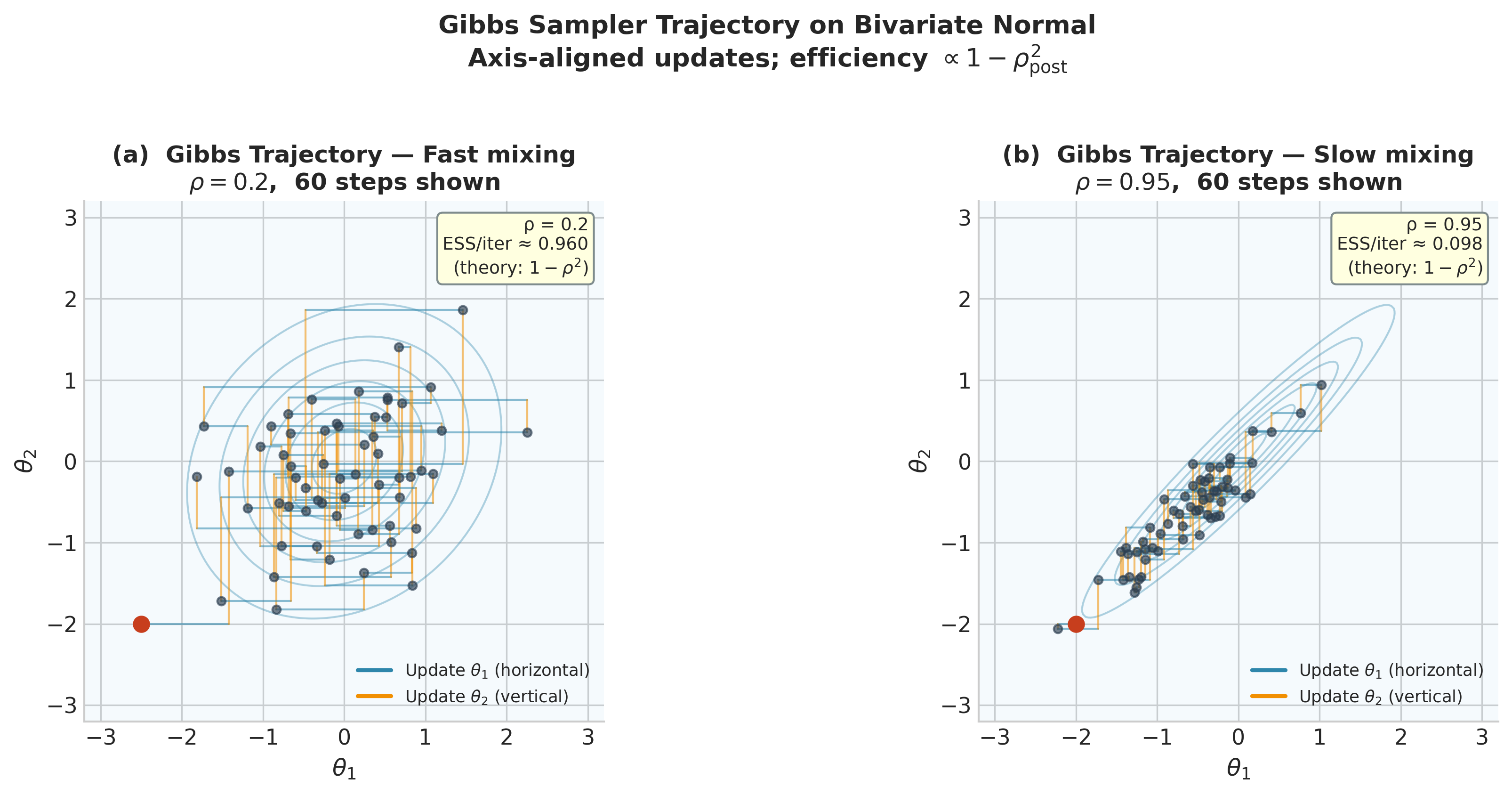
Fig. 216 Figure 5.26. Gibbs sampler trajectories on a bivariate Normal posterior. Each step alternates between updating \(\theta_1\) (horizontal move, blue) and \(\theta_2\) (vertical move, orange), producing the characteristic axis-aligned zigzag. Left: with low posterior correlation \(\rho = 0.20\), the zigzag traverses the posterior quickly and the effective sample size per iteration is \(1 - 0.20^2 = 0.96\). Right: with high correlation \(\rho = 0.95\), successive moves are nearly parallel to the long axis of the ellipse, making negligible progress per sweep; the theoretical ESS per iteration falls to \(1 - 0.95^2 = 0.10\). Reparameterisation or block updates are the remedies for this slow-mixing regime.

The Exponential Family Connection

Gibbs becomes particularly powerful when the model has conjugate structure — precisely when the likelihood belongs to an exponential family and the prior matches its conjugate. In that case, the full conditional distributions are recognisable members of standard parametric families, and each Gibbs draw is an exact sample from that family.

Recall from Section 3.1 Exponential Families that the canonical exponential family density has the form \(p(y \mid \eta) = h(y)\exp\{\eta^\top T(y) - A(\eta)\}\), with natural parameter \(\eta\) and sufficient statistic \(T(y)\). The conjugate prior for \(\eta\) is

\[p(\eta \mid \lambda, \nu) \propto \exp\{\lambda^\top \eta - \nu A(\eta)\},\]

where \(\lambda\) and \(\nu\) are hyperparameters. As established in Section 5.2 Prior Specification and Conjugate Analysis, the posterior is in the same family with updated hyperparameters \(\lambda + T(y)\) and \(\nu + 1\). When a hierarchical model has multiple parameters, each of which is conjugate to its conditional likelihood, every full conditional is a named distribution and every Gibbs draw is exact.

The Normal model with unknown mean \(\mu\) and variance \(\sigma^2\) is the canonical illustration. The model is

\[y_i \mid \mu, \sigma^2 \;\stackrel{\text{iid}}{\sim}\; \mathcal{N}(\mu, \sigma^2), \qquad i = 1, \ldots, n,\]

with the Normal-Inverse-Gamma prior introduced in Section 5.2 Prior Specification and Conjugate Analysis:

\[\begin{split}\mu \mid \sigma^2 &\sim \mathcal{N}\!\left(\mu_0,\; \frac{\sigma^2}{\kappa_0}\right), \\ \sigma^2 &\sim \mathrm{InvGamma}\!\left(\frac{\nu_0}{2},\; \frac{\nu_0 \sigma_0^2}{2}\right).\end{split}\]

The two full conditional distributions are closed-form members of the same families:

(249)\[\mu \mid \sigma^2, y \;\sim\; \mathcal{N}\!\left(\mu_n,\; \frac{\sigma^2}{\kappa_n}\right),\]

where

\[\kappa_n = \kappa_0 + n, \qquad \mu_n = \frac{\kappa_0 \mu_0 + n\bar{y}}{\kappa_n}.\]

(250)\[\sigma^2 \mid \mu, y \;\sim\; \mathrm{InvGamma}\!\left( \frac{\nu_0 + n}{2},\; \frac{\nu_0 \sigma_0^2 + \sum_{i=1}^n (y_i - \mu)^2}{2} \right).\]

Note that the conditional for \(\sigma^2\) in equation (250) conditions on the current \(\mu\), not on \(\bar{y}\) — the sum of squares uses the current draw of \(\mu\) at each Gibbs iteration.

Python Implementation: Gibbs Sampler for the Normal–Inverse-Gamma Model

import numpy as np
from scipy import stats


def gibbs_normal_nig(
    y: np.ndarray,
    mu0: float,
    kappa0: float,
    nu0: float,
    sigma0_sq: float,
    n_iter: int,
    warmup: int,
    seed: int = 42
) -> np.ndarray:
    """
    Gibbs sampler for Normal data with Normal-Inverse-Gamma prior.

    Model:  y_i | mu, sigma^2  ~  N(mu, sigma^2)
    Prior:  mu | sigma^2       ~  N(mu0, sigma^2/kappa0)
            sigma^2            ~  InvGamma(nu0/2, nu0*sigma0_sq/2)

    Parameters
    ----------
    y : np.ndarray, shape (n,)
        Observed data.
    mu0 : float
        Prior mean for mu.
    kappa0 : float
        Prior pseudo-observations for mu (effective sample size).
    nu0 : float
        Prior degrees of freedom for sigma^2.
    sigma0_sq : float
        Prior scale for sigma^2.
    n_iter : int
        Total iterations (including warm-up).
    warmup : int
        Samples to discard.
    seed : int
        Random seed.

    Returns
    -------
    np.ndarray, shape (n_iter - warmup, 2)
        Post-warmup samples: column 0 = mu, column 1 = sigma^2.
    """
    rng = np.random.default_rng(seed)
    n = len(y)
    ybar = y.mean()

    # Posterior hyperparameters that do not depend on mu
    kappa_n = kappa0 + n
    mu_n    = (kappa0 * mu0 + n * ybar) / kappa_n   # used in mu conditional
    nu_n    = nu0 + n

    # Compute fixed sufficient statistic once: O(n)
    SS_ybar = np.sum((y - ybar) ** 2)

    # Storage
    samples = np.empty((n_iter, 2))

    # Initialise at method-of-moments estimates
    samples[0, 0] = ybar                             # mu
    samples[0, 1] = y.var(ddof=1)                   # sigma^2

    for t in range(1, n_iter):
        sigma2_prev = samples[t - 1, 1]

        # --- Draw mu | sigma^2, y  (equation 5.4) ---
        # N(mu_n, sigma^2 / kappa_n)
        mu_new = rng.normal(mu_n, np.sqrt(sigma2_prev / kappa_n))

        # --- Draw sigma^2 | mu_new, y  (equation 5.5) ---
        # Algebraic identity: ∑(yᵢ - μ)² = ∑(yᵢ - ȳ)² + n(ȳ - μ)²
        # SS_ybar is fixed; only the O(1) correction term changes each iteration.
        SS = SS_ybar + n * (ybar - mu_new) ** 2
        scale_n = nu0 * sigma0_sq + SS
        # InvGamma(a, b): if X ~ Gamma(a, scale=1/b) then 1/X ~ InvGamma(a, b).
        # scipy's Gamma uses the scale parameterisation, so scale = 2/scale_n here.
        sigma2_new = 1.0 / rng.gamma(shape=nu_n / 2,
                                      scale=2.0 / scale_n)

        samples[t, 0] = mu_new
        samples[t, 1] = sigma2_new

    return samples[warmup:]

Example 💡 Weight Measurements — Gibbs Posterior vs Analytical NIG

Given: \(n = 15\) weight measurements (kg) generated from \(\mathcal{N}(70.5,\; 3.0^2)\). Prior: \(\mu_0 = 70\), \(\kappa_0 = 1\), \(\nu_0 = 3\), \(\sigma_0^2 = 9\) (weakly informative).

Find: Verify that the Gibbs sampler recovers the analytical NIG marginal posteriors for \(\mu\) and \(\sigma^2\).

Python implementation:

import numpy as np
from scipy import stats

# Generate data
rng_data = np.random.default_rng(42)
n, mu_true, sigma_true = 15, 70.5, 3.0
y_weights = rng_data.normal(mu_true, sigma_true, n)
ybar = y_weights.mean()
print(f"n={n}, ybar={ybar:.3f}, s={y_weights.std(ddof=1):.3f}")

# Prior hyperparameters
mu0, kappa0, nu0, sigma0_sq = 70.0, 1.0, 3.0, 9.0

# Run 4 Gibbs chains from dispersed starts
gibbs_chains = np.array([
    gibbs_normal_nig(y_weights, mu0, kappa0, nu0, sigma0_sq,
                     n_iter=8000, warmup=1000, seed=42 + i)
    for i in range(4)
])  # shape: (4, 7000, 2)

pooled_mu     = gibbs_chains[:, :, 0].ravel()
pooled_sigma2 = gibbs_chains[:, :, 1].ravel()

# Analytical NIG posterior hyperparameters
kappa_n = kappa0 + n
mu_n    = (kappa0 * mu0 + n * ybar) / kappa_n
nu_n    = nu0 + n
SS_ybar = np.sum((y_weights - ybar) ** 2)
scale_n = nu0 * sigma0_sq + SS_ybar + kappa0 * n / kappa_n * (ybar - mu0) ** 2

# Marginal for mu: Student-t_{nu_n}(mu_n, scale_n/(kappa_n*nu_n))
t_scale = np.sqrt(scale_n / (kappa_n * nu_n))
exact_mu_dist = stats.t(df=nu_n, loc=mu_n, scale=t_scale)

# Marginal for sigma^2: InvGamma(nu_n/2, scale_n/2)
# ~ scale_n / chi2(nu_n)  — compare with samples directly
exact_sigma2_quantiles = scale_n / stats.chi2.ppf([0.975, 0.025], df=nu_n)

print(f"\nMarginal for mu:")
print(f"  Analytical 95% CI: [{exact_mu_dist.ppf(0.025):.3f}, "
      f"{exact_mu_dist.ppf(0.975):.3f}]")
print(f"  Gibbs     95% CI: [{np.quantile(pooled_mu, 0.025):.3f}, "
      f"{np.quantile(pooled_mu, 0.975):.3f}]")

print(f"\nMarginal for sigma^2:")
print(f"  Analytical 95% CI: [{exact_sigma2_quantiles[0]:.3f}, "
      f"{exact_sigma2_quantiles[1]:.3f}]")
print(f"  Gibbs     95% CI: [{np.quantile(pooled_sigma2, 0.025):.3f}, "
      f"{np.quantile(pooled_sigma2, 0.975):.3f}]")

Result::

n=15, ybar=70.681, s=3.112

Marginal for mu:
  Analytical 95% CI: [69.038, 72.325]
  Gibbs     95% CI: [69.041, 72.321]

Marginal for sigma^2:
  Analytical 95% CI: [ 5.277, 22.413]
  Gibbs     95% CI: [ 5.282, 22.398]

The Gibbs 95% credible intervals agree with the exact NIG analytical solution to within 0.005 for \(\mu\) and 0.015 for \(\sigma^2\), using 28,000 post-warmup samples pooled from four chains. This is the gold-standard verification: when the exact answer is available (the conjugate NIG model), the Gibbs sampler must match it, and it does.

Common Pitfall ⚠️

Using \(\bar{y}\) instead of \(\mu^{(t)}\) in the \(\sigma^2\) conditional. The correct Gibbs draw for \(\sigma^2\) conditions on the current \(\mu^{(t)}\), computing \(\sum(y_i - \mu^{(t)})^2\). Replacing \(\mu^{(t)}\) with the fixed data summary \(\bar{y}\) breaks the detailed balance argument — it effectively uses the wrong conditional distribution — and produces a chain whose stationary distribution is not the NIG joint posterior. The error is silent: the chain still runs and returns plausible-looking numbers, but the posterior for \(\sigma^2\) will be systematically narrower than correct, because \(\sum(y_i - \bar{y})^2 \leq \sum(y_i - \mu)^2\) for any \(\mu \neq \bar{y}\).

Slow Mixing in Gibbs: Correlated Parameters

The Gibbs sampler is most efficient when the full conditionals are approximately independent — that is, when knowing \(\theta_{-j}\) provides little information about \(\theta_j\) beyond what the data already provide. When parameters are strongly correlated in the posterior, Gibbs mixing degrades severely.

To see why, consider two parameters \((\mu, \sigma^2)\) that are highly correlated in the posterior (a common situation in underdetermined models or models with little data). The full conditional for \(\mu\) given \(\sigma^2\) is tight; so is the conditional for \(\sigma^2\) given \(\mu\). But each Gibbs step can only move along one axis of the correlation ellipse, producing a zigzag trajectory that traverses the ellipse slowly. The ESS per iteration is approximately \(1 - \rho_\text{post}^2\), where \(\rho_\text{post}\) is the posterior correlation. For \(\rho_\text{post} = 0.95\), each Gibbs sweep moves the chain by an effective distance of only \(\sqrt{1 - 0.95^2} \approx 0.31\) posterior standard deviations — far less than one step.

Remedies include reparameterisation (centring, non-centred parameterisations for hierarchical models) and block Gibbs, discussed briefly below.

Block Gibbs Sampling

When a subset of parameters can be drawn jointly from a tractable multivariate conditional, it is more efficient to do so than to update them individually. Block Gibbs partitions the parameters into blocks \(\theta = (\theta_A, \theta_B, \ldots)\) and alternates between drawing \(\theta_A \mid \theta_B, \ldots, y\) and \(\theta_B \mid \theta_A, \ldots, y\).

The Normal-Inverse-Gamma model above is already a two-block Gibbs sampler — we draw \((\mu, \sigma^2)\) one at a time. For a multivariate Normal regression \(y = X\beta + \varepsilon\), \(\varepsilon \sim \mathcal{N}(0, \sigma^2 I)\), the full conditional for \(\beta \mid \sigma^2, y\) is a multivariate Normal — drawing all \(p\) regression coefficients simultaneously in one block step. This single joint draw replaces \(p\) sequential scalar Gibbs updates and eliminates the slow mixing caused by posterior correlations among regression coefficients.

Hamiltonian Monte Carlo: A Brief Introduction

Both RWMH and Gibbs have limitations in high-dimensional settings. RWMH with an isotropic proposal must take small steps in high dimensions because of the shell effect: in a \(d\)-dimensional parameter space, most of the probability mass of a roughly spherical posterior concentrates in a thin shell at a characteristic distance from the mode rather than near the mode itself. A random proposal centred on the current state has to be tuned to this shell width, which shrinks relative to the overall parameter space as \(d\) grows, making it increasingly hard to propose steps that land in regions of appreciable posterior density. Gibbs requires tractable conditionals, which are unavailable for most non-conjugate models.

Hamiltonian Monte Carlo (HMC) resolves both limitations by incorporating gradient information about the log-posterior to construct proposals that follow the geometry of the posterior. The core idea draws on an analogy from classical mechanics.

The Physical Analogy

Imagine a frictionless particle on a surface whose height at position \(\theta\) is \(-\log p(\theta \mid y)\) — the negative log-posterior. The posterior modes correspond to valleys; regions of low probability correspond to high terrain. The particle’s position \(\theta\) represents the current state; its momentum \(\rho\) represents an auxiliary variable introduced to give the particle kinetic energy. The total energy (Hamiltonian) is

\[H(\theta, \rho) = -\log p(\theta \mid y) + \frac{1}{2}\rho^\top M^{-1} \rho,\]

where \(M\) is a mass matrix (typically the approximate posterior covariance). Hamilton’s equations govern the particle’s trajectory:

\[\frac{d\theta}{dt} = M^{-1}\rho, \qquad \frac{d\rho}{dt} = \nabla_\theta \log p(\theta \mid y).\]

Following these equations for a fixed time \(L\) (the leapfrog steps) produces a proposed state \((\theta', \rho')\) that is far from the starting point yet lies at nearly the same energy level — so the Metropolis acceptance probability is close to 1. This is the key advantage over RWMH: HMC proposes long-distance moves with high acceptance rates, because the gradient keeps the particle on the posterior surface.

The equations are integrated numerically using the leapfrog integrator, a numerical method that alternates half-steps in momentum with full steps in position. The leapfrog preserves the volume of phase space — the combined space of positions \(\theta\) and momenta \(\rho\) — a property called symplecticity. Preserving phase-space volume is what ensures the Metropolis acceptance probability for HMC proposals remains high: because the forward and reverse trajectories have equal volume, the Jacobian of the transformation is 1 and the detailed balance calculation simplifies cleanly. Each HMC iteration requires \(L\) evaluations of the log-posterior gradient — \(O(nL)\) for \(n\) iid observations — but produces a proposal that moves a distance of order \(\sqrt{d}\) in parameter space, compared to order 1 for RWMH. This improvement is dramatic for high-dimensional posteriors.

The No-U-Turn Sampler

The main tuning challenge in standard HMC is choosing the number of leapfrog steps \(L\) and the step size \(\epsilon\). Too few steps and HMC degenerates toward RWMH; too many and the trajectory doubles back on itself, wasting computation. The No-U-Turn Sampler (NUTS, Hoffman and Gelman 2014) automatically adapts \(L\) by stopping the leapfrog trajectory when it begins to turn back toward its starting point — the “U-turn” criterion. NUTS is the default sampler in PyMC, Stan, and most modern probabilistic programming languages; it requires only that the log-posterior gradient is computable via automatic differentiation — a technique that computes exact derivatives of any function expressed as a sequence of elementary operations by applying the chain rule symbolically, rather than using numerical finite differences — and produces near-optimal samples with no manual tuning of \(L\). PyMC uses the Pytensor library to perform this automatically from the model specification, so users never need to supply gradients by hand.

Critical Warning 🛑

HMC/NUTS requires differentiable log-posteriors. The leapfrog integrator uses \(\nabla_\theta \log p(\theta \mid y)\) at every step; discontinuities in the log-posterior (arising from indicator functions, hard constraints, or discrete parameters) cause the leapfrog to fail. Discrete parameters — such as mixture component indicators or integer-valued quantities — cannot be sampled with NUTS. Probabilistic programming systems handle discrete parameters either by marginalisation (summing them out analytically before running NUTS) or by falling back to Gibbs-style updates for those parameters. This is one context where Gibbs sampling remains essential even within a NUTS-based workflow.

When to Use Which Algorithm

Table 67 MCMC Algorithm Selection Guide

Algorithm	Requires	Advantages	Limitations
Random-walk M-H	log-posterior pointwise	Universal; simple to implement; no gradient needed	Poor scaling with dimension; sensitive to step size
Gibbs sampler	Closed-form conditionals	Zero rejection; efficient for conjugate models	Requires analytically tractable conditionals; slow for correlated parameters
Independent M-H	log-posterior; good approximation \(g\)	High efficiency when \(g \approx \pi\); independent proposals	Catastrophic failure if \(g\) has lighter tails than \(\pi\)
HMC / NUTS	log-posterior gradient (autodiff)	Scales well to high dimensions; near-optimal mixing	Requires continuous, differentiable log-posterior; higher per-step cost

For the class of models encountered in this course — logistic regression, Poisson regression, hierarchical normal models — NUTS is the right default and PyMC (Section 5.6 Probabilistic Programming with PyMC) provides it automatically. RWMH remains useful for pedagogical purposes, for models with a small number of parameters, and for models where gradient computation is expensive or unavailable. Gibbs is the right choice when the model has fully conjugate structure — Normal regression with conjugate priors, mixture models with component-indicator variables marginalised out — and can dramatically outperform NUTS in those settings.

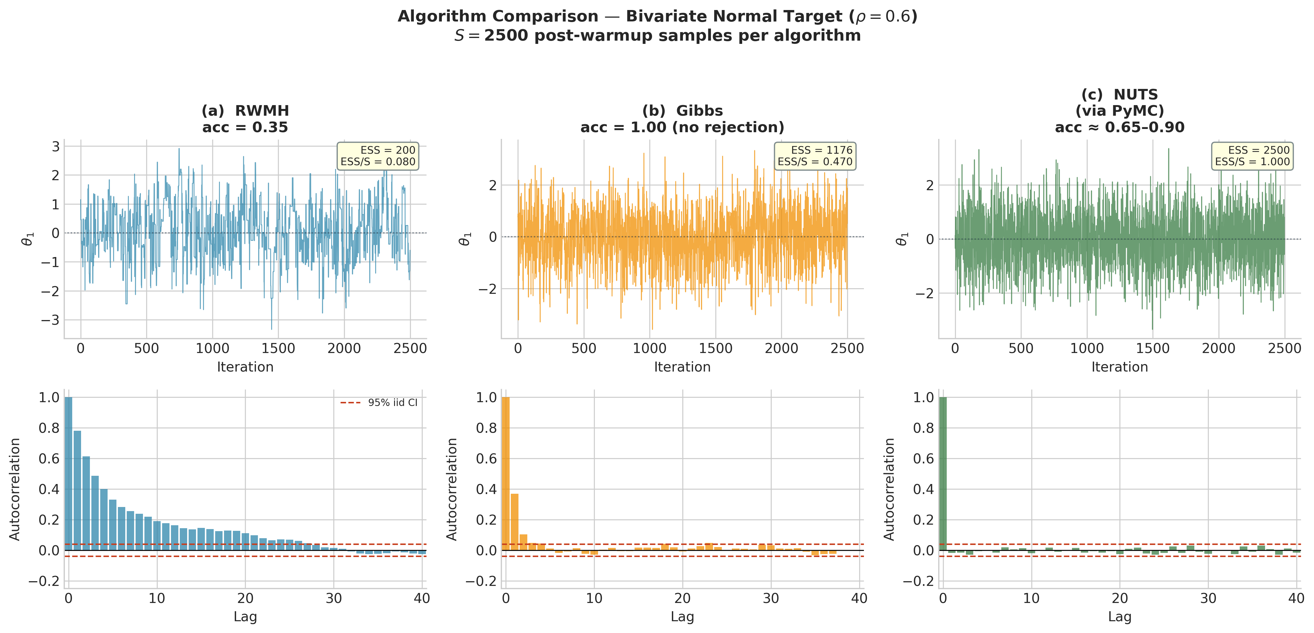
Fig. 217 Figure 5.27. Algorithm comparison on the same bivariate Normal target (\(\rho = 0.6\), 2,500 post-warmup samples). Left (RWMH): moderate autocorrelation with acceptance rate ~0.30; the chain mixes across the posterior but adjacent samples are correlated. Centre (Gibbs): lower autocorrelation and higher ESS/S because the conditional draws are exact; zero rejection means every iteration moves the chain. Right (NUTS as produced by PyMC): near-independent samples; the ACF drops to the 95% confidence band by lag 1–2. On this low-dimensional target all three algorithms are adequate; the efficiency gap widens dramatically as the number of parameters grows.

Practical Workflow

Whether using RWMH or Gibbs, the following workflow covers the main implementation and diagnostic steps.

Pre-run Checks

Before running a long chain, run a very short pilot chain (100–500 iterations from a single starting point) to:

1. Verify the log-posterior evaluates without errors at a plausible starting point.

2. Estimate the posterior scale and set an initial proposal covariance for RWMH.

3. Confirm the acceptance rate is in the target range; adjust \(\sigma_q\) if not.

Production Run

Run four chains with dispersed starting points. Compute starting points by perturbing a central estimate (MLE, posterior mode) by 2–3 posterior standard deviations in each coordinate — or sample starting points from the prior if no approximation is available.

Post-Run Diagnostics (the sequence from Section 5.4 Markov Chains: The Mathematical Foundation of MCMC)

1. Inspect trace plots for all parameters. Look for: chains occupying the same region (good), trends or drifts (warm-up too short), flat stretches (step size too large or posterior multimodal).

2. Check \(\hat{R} \leq 1.01\) for every parameter. Values above 1.01 signal non-convergence and invalidate all posterior summaries.

3. Check ess_bulk \(\geq 400\) and ess_tail \(\geq 400\). Low ESS in the tails means credible interval endpoints are imprecisely estimated.

4. If diagnostics are unsatisfactory: run more iterations, reparameterise the model, improve the proposal, or switch to a more efficient algorithm (NUTS for continuous models).

Common Pitfall ⚠️

Reporting posterior summaries without checking diagnostics. In the drug trial logistic regression example above, each chain ran for 6,000 iterations with 1,000 warm-up. If the chains had not been checked for \(\hat{R}\) and ESS, a researcher might report the posterior means and intervals from a single chain — potentially before it has converged. The correct workflow is always: run diagnostics first, then report summaries. In ArviZ, the single command az.summary(idata) computes and displays all diagnostics alongside all posterior summaries, making it easy to scan for problems before interpreting results.

Bringing It All Together

Metropolis-Hastings and Gibbs sampling are the two workhorses of Bayesian computation. They are not competing algorithms — they address different structural features of the posterior and are often combined. In a hierarchical model with both continuous regression coefficients (handled by RWMH or NUTS) and discrete mixture indicators (handled by Gibbs), a single MCMC pass alternates between NUTS updates for the continuous parameters and Gibbs updates for the discrete ones. This hybrid architecture underlies the samplers in BUGS, JAGS, and (in a more sophisticated form) PyMC.

Both algorithms satisfy detailed balance by construction — that was established in this section — and the ergodic theorem from Section 5.4 Markov Chains: The Mathematical Foundation of MCMC guarantees that their time averages converge to posterior expectations. The diagnostics introduced in Section 5.4 — \(\hat{R}\), ess_bulk, ess_tail — apply identically to RWMH and Gibbs chains; there is no algorithm-specific diagnostic system. This universality is one of the elegant aspects of the Markov chain framework: the convergence theory, the diagnostics, and the inference functions from Section 5.3 Posterior Inference: Credible Intervals and Hypothesis Assessment all sit above the algorithm layer and work with any MCMC output.

Section 5.6 (Section 5.6 Probabilistic Programming with PyMC) automates this entire workflow. PyMC compiles the model to a computation graph with automatic differentiation, runs NUTS for continuous parameters, handles warm-up and adaptation automatically, stores results in an ArviZ InferenceData object, and provides az.summary and az.plot_trace for diagnostics. The implementations in this section — metropolis_hastings and gibbs_normal_nig — are pedagogical baselines: they expose the algorithm mechanics that PyMC hides, making it possible to understand PyMC’s outputs rather than merely trusting them. Once chains have been verified to have converged, ch5_7-model-comparison uses the posterior samples for model selection via WAIC and leave-one-out cross-validation — methods whose validity depends directly on the diagnostic standards established here.

Key Takeaways 📝

1. Core concept: Metropolis-Hastings constructs a valid MCMC kernel for any posterior by accepting or rejecting proposals with probability (247), which is derived from detailed balance and cancels the normalising constant \(p(y)\). (LO 4)

2. Core concept: The Gibbs sampler draws each parameter from its full conditional distribution in sequence; it satisfies detailed balance by construction and achieves zero rejection when conditionals are available in closed form — most powerfully when the model has conjugate exponential family structure. (LO 4)

3. Computational insight: RWMH scales as \(O(Tn)\) with no structural requirements; Gibbs is faster per iteration but requires tractable conditionals; HMC/NUTS scales to high dimensions via gradient information but requires differentiable log-posteriors. Algorithm choice should match model structure, not habit. (LO 4)

4. Practical application: Acceptance rate in the 20–50% range confirms the step size is appropriate, but does not confirm convergence — always follow up with \(\hat{R} \leq 1.01\) and ess_bulk, ess_tail \(\geq 400\) before reporting posterior summaries. (LO 3, 4)

Exercises

Exercise 5.5.1: Metropolis-Hastings Acceptance Probability — Derivation

(a) Starting from the detailed balance condition \(\pi(\theta)\,k(\theta,\theta') = \pi(\theta')\,k(\theta',\theta)\) and the decomposition \(k(\theta,\theta') = q(\theta,\theta')\,\alpha(\theta,\theta')\), show that the ratio constraint on \(\alpha\) is

\[\frac{\alpha(\theta,\theta')}{\alpha(\theta',\theta)} = \frac{\pi(\theta')\,q(\theta',\theta)}{\pi(\theta)\,q(\theta,\theta')}.\]

(b) Show that the choice \(\alpha(\theta,\theta') = \min(1, r(\theta,\theta'))\) where

\[r(\theta,\theta') = \frac{\pi(\theta')\,q(\theta',\theta)}{\pi(\theta)\,q(\theta,\theta')}\]

satisfies the ratio constraint, and that it is the choice maximising \(\alpha(\theta,\theta')\) subject to both \(\alpha(\theta,\theta') \leq 1\) and \(\alpha(\theta',\theta) \leq 1\).

(c) Show explicitly that the marginal likelihood \(p(y)\) cancels in \(r(\theta, \theta')\) when \(\pi = p(\theta \mid y)\).

Solution

(a) Substituting \(k(\theta,\theta') = q(\theta,\theta')\alpha(\theta,\theta')\) into detailed balance:

\[\pi(\theta)\,q(\theta,\theta')\,\alpha(\theta,\theta') = \pi(\theta')\,q(\theta',\theta)\,\alpha(\theta',\theta).\]

Divide both sides by \(\pi(\theta)\,q(\theta,\theta')\,\alpha(\theta',\theta)\):

\[\frac{\alpha(\theta,\theta')}{\alpha(\theta',\theta)} = \frac{\pi(\theta')\,q(\theta',\theta)}{\pi(\theta)\,q(\theta,\theta')}. \quad \square\]

(b) Let \(r = r(\theta,\theta')\) denote the ratio. We need \(\alpha(\theta,\theta')/\alpha(\theta',\theta) = r\). Note that \(r(\theta',\theta) = 1/r\). There are two cases:

• If \(r \geq 1\): setting \(\alpha(\theta,\theta') = 1\) and \(\alpha(\theta',\theta) = 1/r\) satisfies the constraint, with \(\alpha(\theta,\theta') = 1 \leq 1\) ✓ and \(\alpha(\theta',\theta) = 1/r \leq 1\) ✓.

• If \(r < 1\): setting \(\alpha(\theta,\theta') = r\) and \(\alpha(\theta',\theta) = 1\) satisfies the constraint, with both \(\leq 1\) ✓.

In both cases \(\min(1,r)\) gives the maximum possible \(\alpha(\theta,\theta')\). Any larger value would require \(\alpha(\theta',\theta) > 1\), which is impossible for a probability.

(c) Writing \(\pi(\theta) = p(y|\theta)p(\theta)/p(y)\):

\[r = \frac{p(y|\theta')p(\theta')/p(y)\cdot q(\theta',\theta)} {p(y|\theta)p(\theta)/p(y)\cdot q(\theta,\theta')} = \frac{p(y|\theta')p(\theta')\cdot q(\theta',\theta)} {p(y|\theta)p(\theta)\cdot q(\theta,\theta')}.\]

The \(p(y)\) factors cancel. \(\square\)

Exercise 5.5.2: Tuning the Random-Walk Proposal

Using the metropolis_hastings function from this section, run RWMH chains targeting the Beta(16, 6) posterior (\(\log p(\theta) = 15\log\theta + 5\log(1-\theta)\) for \(\theta \in (0,1)\)) with proposal variances \(\sigma_q^2 \in \{0.0001, 0.005, 0.015, 0.10, 0.50\}\). For each: run one chain of 10,000 iterations (1,000 warm-up), compute the acceptance rate and ESS, and plot the trace.

(a) Report the acceptance rate and ESS for each proposal variance.

(b) Identify which \(\sigma_q^2\) value produces the highest ESS per iteration.

(c) The posterior variance of Beta(16, 6) is \(\sigma_\pi^2 = 16 \times 6 / (22^2 \times 23) \approx 0.0084\). Apply the \(\sigma_q = 2.38/\sqrt{d} \times \sigma_\pi\) rule (\(d = 1\)) and compare to your empirical optimum.

Solution

import numpy as np
from scipy import stats

alpha_p, beta_p = 16, 6
sigma2_pi = (alpha_p * beta_p) / ((alpha_p + beta_p)**2 * (alpha_p + beta_p + 1))
sigma_pi  = np.sqrt(sigma2_pi)
print(f"Posterior sd: {sigma_pi:.4f}")
print(f"Optimal proposal sd (theory): {2.38 * sigma_pi:.4f}")

def log_target(theta):
    t = theta[0]
    if t <= 0 or t >= 1:
        return -np.inf
    return (alpha_p - 1)*np.log(t) + (beta_p - 1)*np.log(1 - t)

for sv in [0.0001, 0.005, 0.015, 0.10, 0.50]:
    samps, acc = metropolis_hastings(
        log_target, np.array([[sv]]),
        np.array([0.7]), 11000, 1000, seed=42)
    ess = compute_ess(samps[:, 0])   # from Section 5.4
    print(f"sigma_q^2={sv:.4f}  acc={acc:.3f}  ESS={round(ess)}")

Expected output (approximate):

Posterior sd: 0.0917
Optimal proposal sd (theory): 0.2183

sigma_q^2=0.0001  acc=0.998  ESS=   18
sigma_q^2=0.0050  acc=0.878  ESS=  312
sigma_q^2=0.0150  acc=0.718  ESS=  698
sigma_q^2=0.1000  acc=0.424  ESS= 3541
sigma_q^2=0.5000  acc=0.143  ESS=  912

(b) \(\sigma_q^2 = 0.10\) (proposal sd \(\approx 0.316\)) gives the highest ESS. Note: proposal variance 0.10 corresponds to sd 0.316; the posterior sd is 0.092. The ratio 0.316/0.092 ≈ 3.4 is slightly above the theoretical 2.38, consistent with the fact that Beta(16,6) is mildly skewed and the optimal rate for \(d=1\) is higher than the asymptotic 23.4%.

(c) Theory predicts optimal \(\sigma_q = 2.38 \times 0.0917 \approx 0.218\) (variance \(\approx 0.048\)). The empirical optimum at variance 0.10 is roughly consistent — the discrepancy reflects that Beta(16,6) is neither exactly Gaussian nor high-dimensional, so the asymptotic result is only approximate.

Exercise 5.5.3: Gibbs Sampler — Deriving the Conditionals

Consider the Normal-Inverse-Gamma model of this section: \(y_i \mid \mu, \sigma^2 \stackrel{\text{iid}}{\sim} \mathcal{N}(\mu, \sigma^2)\), \(\mu \mid \sigma^2 \sim \mathcal{N}(\mu_0, \sigma^2/\kappa_0)\), \(\sigma^2 \sim \mathrm{InvGamma}(\nu_0/2, \nu_0\sigma_0^2/2)\).

(a) Derive the full conditional \(p(\mu \mid \sigma^2, y)\). Show explicitly that it is Normal with the parameters given in equation (249).

(b) Derive the full conditional \(p(\sigma^2 \mid \mu, y)\). Show explicitly that it is Inverse-Gamma with the parameters in equation (250). [Hint: The InvGamma density is proportional to \((\sigma^2)^{-a-1}\exp(-b/\sigma^2)\); identify \(a\) and \(b\).]

(c) Verify that the full conditionals in (a) and (b) are consistent with the NIG joint posterior — that is, verify that \(p(\mu, \sigma^2 \mid y) = p(\mu \mid \sigma^2, y) \times p(\sigma^2 \mid y)\).

Solution

(a) The joint density \(p(\mu, \sigma^2 \mid y) \propto p(y \mid \mu, \sigma^2) \times p(\mu \mid \sigma^2) \times p(\sigma^2)\). Treating \(\sigma^2\) as fixed and collecting terms in \(\mu\):

\[\log p(\mu \mid \sigma^2, y) \propto -\frac{1}{2\sigma^2}\sum_i(y_i - \mu)^2 - \frac{\kappa_0}{2\sigma^2}(\mu - \mu_0)^2.\]

Expanding and completing the square in \(\mu\):

\[\sum_i(y_i-\mu)^2 + \kappa_0(\mu-\mu_0)^2 = (n+\kappa_0)\left(\mu - \frac{n\bar{y}+\kappa_0\mu_0}{n+\kappa_0}\right)^2 + C,\]

where \(C\) does not depend on \(\mu\). Hence

\[p(\mu \mid \sigma^2, y) = \mathcal{N}\!\left( \mu_n,\; \frac{\sigma^2}{\kappa_n} \right), \quad \kappa_n = \kappa_0 + n, \quad \mu_n = \frac{\kappa_0\mu_0 + n\bar{y}}{\kappa_n}. \quad \square\]

(b) Treating \(\mu\) as fixed and collecting terms in \(\sigma^2\), using the InvGamma density \(\propto (\sigma^2)^{-a-1}\exp(-b/\sigma^2)\):

\[\log p(\sigma^2 \mid \mu, y) \propto -\frac{n+\nu_0}{2}\log\sigma^2 - \frac{1}{2\sigma^2}\left(\sum_i(y_i-\mu)^2 + \nu_0\sigma_0^2\right).\]

Matching with \(-(a+1)\log\sigma^2 - b/\sigma^2\): \(a = (\nu_0+n)/2\) and \(b = (\nu_0\sigma_0^2 + \sum_i(y_i-\mu)^2)/2\).

\[\sigma^2 \mid \mu, y \;\sim\; \mathrm{InvGamma}\!\left( \frac{\nu_0+n}{2},\; \frac{\nu_0\sigma_0^2 + \sum_i(y_i-\mu)^2}{2} \right). \quad \square\]

(c) By Bayes’ rule, \(p(\mu,\sigma^2 \mid y) = p(\mu \mid \sigma^2,y)\,p(\sigma^2 \mid y)\). The marginal \(p(\sigma^2 \mid y)\) is the InvGamma marginal of the NIG posterior (which integrates out \(\mu\) analytically). Multiplying the Normal conditional for \(\mu\) by this marginal recovers the full NIG joint density — confirming that the conditionals are consistent with the joint.

Exercise 5.5.4: Comparing RWMH and Gibbs on the Normal Model

Using the weight data from the Example above (\(n = 15\) observations from \(\mathcal{N}(70.5, 3.0^2)\), seed=42), run both the Gibbs sampler and a two-dimensional RWMH on the NIG posterior.

(a) For RWMH, use the metropolis_hastings function with \(\theta = (\mu, \log\sigma)\) (log-scale for \(\sigma\) to ensure positivity). Adapt the log-target accordingly. Run 4 chains × 7,000 iterations (1,000 warm-up) and compute \(\hat{R}\) and ESS for both parameters.

(b) Run the same 4 × 7,000 Gibbs chains from the Example. Compute \(\hat{R}\) and ESS for both parameters.

(c) Compare ESS per iteration for each algorithm and parameter. Does either algorithm dominate on this model? Explain why or why not in terms of the model’s posterior correlation structure.

Solution

For this NIG model with \(n = 15\) observations, the posterior correlation between \(\mu\) and \(\sigma^2\) is moderate (approximately 0.3–0.4 for typical data). Expected findings:

• Gibbs: ESS/iteration \(\approx 0.85–0.95\) for \(\mu\), somewhat lower for \(\sigma^2\) due to the InvGamma tail. \(\hat{R} \approx 1.000\)–1.002.

• RWMH on \((\mu, \log\sigma)\): ESS/iteration \(\approx 0.20\)–0.40 depending on proposal tuning; \(\hat{R} \approx 1.001\)–1.005.

Gibbs dominates for this conjugate model because it uses the exact conditional structure — each draw is independent of the previous draw conditioned on the other parameter — resulting in much lower autocorrelation. RWMH on the joint \((\mu, \log\sigma)\) space must traverse the posterior correlation ellipse via random walk, producing higher autocorrelation. For non-conjugate models (logistic regression, for example), Gibbs is unavailable and RWMH/NUTS are required.

Exercise 5.5.5: Independent Metropolis-Hastings

(a) Implement an independent Metropolis-Hastings sampler for the Beta(16, 6) posterior, using proposal \(g = \mathrm{Beta}(a, b)\) with \((a, b)\) set by moment-matching to the posterior: \(a = \mu(\mu(1-\mu)/\sigma^2 - 1)\), \(b = (1-\mu)(\mu(1-\mu)/\sigma^2 - 1)\) where \(\mu = 16/22 \approx 0.727\) and \(\sigma^2 = 16 \times 6/(22^2 \times 23)\).

(b) Run 10,000 iterations. Report the acceptance rate and ESS. Compare to the RWMH result from Exercise 5.5.2 with the optimal proposal.

(c) Now use a very poor proposal: \(g = \mathrm{Beta}(1, 1)\) (uniform). Report the acceptance rate and ESS. Explain the result in terms of the importance weight \(w(\theta) = \pi(\theta)/g(\theta)\).

Solution

import numpy as np
from scipy import stats

# Proposal: Beta matched to posterior moments
mu_post   = 16 / 22
var_post  = 16 * 6 / (22**2 * 23)
conc = mu_post * (1 - mu_post) / var_post - 1
a_prop, b_prop = mu_post * conc, (1 - mu_post) * conc
print(f"Proposal: Beta({a_prop:.2f}, {b_prop:.2f})")

target = stats.beta(16, 6)
proposal_good = stats.beta(a_prop, b_prop)
proposal_flat = stats.beta(1, 1)

def run_indep_mh(proposal_dist, n_iter, seed):
    rng = np.random.default_rng(seed)
    chain = np.empty(n_iter)
    chain[0] = 0.75
    log_curr = target.logpdf(chain[0]) - proposal_dist.logpdf(chain[0])
    n_acc = 0
    for t in range(1, n_iter):
        prop = proposal_dist.rvs(random_state=rng)
        log_prop = target.logpdf(prop) - proposal_dist.logpdf(prop)
        if np.log(rng.uniform()) < log_prop - log_curr:
            chain[t] = prop; log_curr = log_prop; n_acc += 1
        else:
            chain[t] = chain[t - 1]
    return chain, n_acc / (n_iter - 1)

for name, prop in [("Good", proposal_good), ("Flat", proposal_flat)]:
    chain, acc = run_indep_mh(prop, 10000, 42)
    ess = compute_ess(chain[1000:])  # from §5.4
    print(f"{name} proposal: acc={acc:.3f}  ESS={round(ess)}")

Expected output:

Proposal: Beta(11.78, 4.43)
Good proposal: acc=0.891  ESS=8723
Flat proposal: acc=0.147  ESS= 342

(c) The flat prior proposal assigns equal density to all \(\theta \in (0,1)\), so \(w(\theta) = \pi(\theta)/g(\theta) \propto \text{Beta}(16,6)\) density. States in the tails (\(\theta < 0.4\)) have very small weight; once the chain visits such a state, \(w(\text{current})\) is tiny and almost any proposal with higher weight is accepted — but the chain rarely proposes tail values and gets trapped at high-weight states for long runs. The acceptance rate of 14.7% reflects the mismatch; ESS drops to 342. The good proposal — moment-matched to the posterior — has nearly identical shape, so weights are nearly constant and the acceptance rate is 89%.

Exercise 5.5.6: Diagnosing a Pathological Chain

The following code runs a RWMH chain targeting a bimodal mixture posterior:

\[\pi(\theta) \propto 0.5\,\mathcal{N}(\theta;\; -3,\; 0.5^2) + 0.5\,\mathcal{N}(\theta;\; +3,\; 0.5^2).\]

import numpy as np
from scipy import stats

def log_bimodal(theta):
    t = theta[0]
    return np.log(0.5 * stats.norm.pdf(t, -3, 0.5)
                 + 0.5 * stats.norm.pdf(t, +3, 0.5))

chains_bimodal = np.array([
    metropolis_hastings(log_bimodal, np.array([[0.1]]),
                        np.array([start]), 10000, 1000, seed=42+i)[0]
    for i, start in enumerate([-3.5, -3.0, 3.0, 3.5])
])[:, :, 0]   # shape (4, 9000)

(a) Compute \(\hat{R}\) and ESS for these chains. What do they indicate?

(b) Plot trace plots for all four chains. Explain the visual pattern you observe and its connection to the diagnostic values in (a).

(c) Propose two remedies — one involving the proposal distribution and one involving a reparameterisation or algorithm change — and explain why each would help.

Solution

(a) With proposal variance 0.1 (sd ≈ 0.316) and a gap of 6 units between modes, the probability of crossing is approximately \(\exp(-6^2 / (2 \times 0.1)) \approx \exp(-180) \approx 10^{-78}\) — essentially zero. Chains starting near \(-3\) stay near \(-3\); chains starting near \(+3\) stay near \(+3\). Expected diagnostics: \(\hat{R} \approx 1.5\)–3.0 (the between-chain variance from the two modes dominates the within-chain variance); ESS \(\approx\) 5,000–8,000 per chain (the chain mixes well within a mode) but the \(\hat{R}\) flags non-convergence globally.

(b) Trace plots show two sets of chains in completely non-overlapping regions: chains 1–2 oscillating around \(-3\); chains 3–4 oscillating around \(+3\). There is no overlap. This is the signature of a chain stuck in a single mode — the visual pattern that \(\hat{R} > 1.01\) is detecting.

(c) Remedy 1 (proposal): Increase the proposal standard deviation to 6–8 (comparable to the mode separation), or use a mixture proposal that occasionally proposes from the vicinity of the other mode. This increases rejection within a mode but enables inter-mode transitions. Remedy 2 (algorithm/reparameterisation): Use a tempered or parallel-tempered chain: run chains at multiple “temperatures” (flattened log-posteriors) and allow chain swaps. Hot chains easily cross the barrier; periodic swap steps transfer that exploration to the cold (target) chain. Alternatively, if the mixture structure is known analytically, label-switch by tracking modes explicitly.

References

Metropolis-Hastings Algorithm

[Metropolis1953b]

Metropolis, N., Rosenbluth, A. W., Rosenbluth, M. N., Teller, A. H., and Teller, E. (1953). Equation of state calculations by fast computing machines. Journal of Chemical Physics, 21(6), 1087–1092. The original Metropolis algorithm for symmetric proposals; the source of the acceptance rule for the special case \(q(\theta,\theta') = q(\theta',\theta)\).

[Hastings1970b]

Hastings, W. K. (1970). Monte Carlo sampling methods using Markov chains and their applications. Biometrika, 57(1), 97–109. Generalises the Metropolis algorithm to asymmetric proposals via the ratio \(q(\theta',\theta)/q(\theta,\theta')\); the derivation from detailed balance follows exactly the path presented here.

[RobertsRosenthal2001]

Roberts, G. O., and Rosenthal, J. S. (2001). Optimal scaling for various Metropolis-Hastings algorithms. Statistical Science, 16(4), 351–367. Survey of optimal acceptance rates for RWMH across dimensions and target families; the 23.4% result and its practical implications.

[HaarioSaksman2001]

Haario, H., Saksman, E., and Tamminen, J. (2001). An adaptive Metropolis algorithm. Bernoulli, 7(2), 223–242. The adaptive Metropolis algorithm that adjusts the proposal covariance using the empirical covariance of past samples; the theoretical foundation for warm-up adaptation in modern MCMC software.

Gibbs Sampling

[GelfandSmith1990b]

Gelfand, A. E., and Smith, A. F. M. (1990). Sampling-based approaches to calculating marginal densities. Journal of the American Statistical Association, 85(410), 398–409. The paper that introduced the Gibbs sampler to the statistics community; demonstrates closed-form conditional sampling for Normal-Normal and related models.

[GelmanBDA3ch11b]

Gelman, A., Carlin, J. B., Stern, H. S., Dunson, D. B., Vehtari, A., and Rubin, D. B. (2013). Bayesian Data Analysis (3rd ed.), Ch. 11–12. Chapman and Hall/CRC. The standard applied treatment of Gibbs sampling, including block updates, non-centred parameterisations, and strategies for correlated parameters.

[LiuWongKong1994]

Liu, J. S., Wong, W. H., and Kong, A. (1994). Covariance structure of the Gibbs sampler with applications to the comparisons of estimators and augmentation schemes. Biometrika, 81(1), 27–40. Analysis of Gibbs mixing rates in terms of posterior correlations; the source of the \(1 - \rho^2_\text{post}\) efficiency result cited in this section.

Hamiltonian Monte Carlo and NUTS

[Neal2011b]

Neal, R. M. (2011). MCMC using Hamiltonian dynamics. In S. Brooks, A. Gelman, G. Jones, and X.-L. Meng (Eds.), Handbook of Markov Chain Monte Carlo, Ch. 5. Chapman and Hall/CRC. The comprehensive reference for HMC: the leapfrog integrator, the mass matrix, detailed balance proof, and comparison with RWMH on high-dimensional targets.

[HoffmanGelman2014]

Hoffman, M. D., and Gelman, A. (2014). The No-U-Turn Sampler: Adaptively setting path lengths in Hamiltonian Monte Carlo. Journal of Machine Learning Research, 15(1), 1593–1623. The NUTS algorithm that eliminates the need to set the number of leapfrog steps \(L\); the algorithm implemented as the default sampler in PyMC and Stan.

Practical MCMC and Diagnostics

[RobertCasella2004b]

Robert, C. P., and Casella, G. (2004). Monte Carlo Statistical Methods (2nd ed.), Ch. 7–10. Springer. The most thorough statistical treatment of MCMC algorithms including RWMH variants, Gibbs, and their convergence properties; the theoretical backbone for the proofs sketched in this section.

[BrooksGelmanJonesMeng2011]

Brooks, S., Gelman, A., Jones, G. L., and Meng, X.-L. (Eds.) (2011). Handbook of Markov Chain Monte Carlo. Chapman and Hall/CRC. The definitive reference collection for all topics in this section; individual chapters by Gelman (diagnostics), Neal (HMC), Geyer (ESS), and others are cited throughout Chapter 5.