Appendix C: Numerical Analysis Review
From Exact to Approximate
Most statistical computations cannot be done in closed form. Maximum likelihood requires solving nonlinear score equations. Bayesian posteriors require intractable integrals. Confidence intervals require finding roots of profile likelihood functions. Numerical analysis provides the algorithms that turn these mathematical expressions into numbers — and, crucially, the error bounds and convergence guarantees that tell us when to trust those numbers.
This appendix develops the numerical foundations that the rest of the course assumes. We explain why the standard algorithms work (convergence theory, contraction mappings), when they fail (floating-point arithmetic, saddle points, ill-conditioning), and how fast they converge (linear vs quadratic rates). The specific applications of these tools — Newton-Raphson for MLE in Ch3.2, IRLS for GLMs in Ch3.5, quadrature vs Monte Carlo in Ch2.1 — live in the chapters. This appendix provides the engine under the hood.
Road Map 🧭
Section 1 (Floating-Point): IEEE 754 representation, machine epsilon, catastrophic cancellation, log-space arithmetic — the source of most “mysterious” numerical errors
Section 2 (Root Finding): Fixed-point iteration, contraction mapping theorem, bisection, Newton’s method — the framework that unifies all iterative algorithms
Section 3 (Optimization): Gradient descent, Newton’s method for optimization, quasi-Newton — why some algorithms converge in 5 steps and others need 500
Section 4 (Differentiation): Finite differences, optimal step size, the complex-step method — computing derivatives when formulas are unavailable
Section 5 (Integration): Quadrature error theory, adaptive quadrature, Monte Carlo — choosing the right tool for numerical integrals
Section 6 (Convergence): Convergence orders, stopping criteria, diagnosing failure — knowing when to stop and when something has gone wrong
Prerequisites Check
This appendix assumes familiarity with:
Single-variable calculus: Taylor’s theorem and basic derivatives (Appendix A)
Linear algebra basics: Eigenvalues, matrix inverse, solving linear systems (Appendix B)
Python/NumPy: Basic array operations (Appendix F)
Connection to Course Material
Chapter 2 (Monte Carlo): Quadrature vs Monte Carlo convergence rates (Ch2.1), Brent’s method for inverse CDF (Ch2.3), logsumexp for importance weights (Ch2.6)
Chapter 3 (Parametric Inference): Newton-Raphson and Fisher scoring for MLE (Ch3.2), numerical Hessians for standard errors (Ch3.3), IRLS for GLMs (Ch3.5)
Chapter 5 (Bayesian): HMC leapfrog integrator step size (Ch5.5)
Appendix B: Condition numbers and numerical stability of matrix computations
Floating-Point Arithmetic
IEEE 754 Basics
Definition
A floating-point number in IEEE 754 double precision (float64) is stored as \((-1)^s \times 1.m \times 2^{e-1023}\), where \(s\) is a sign bit, \(m\) is a 52-bit mantissa (significand), and \(e\) is an 11-bit exponent. This gives approximately 15–16 significant decimal digits.
Definition
Machine epsilon \(\varepsilon_{\text{mach}}\) is the smallest \(\varepsilon > 0\) such that \(\text{fl}(1 + \varepsilon) \ne 1\) in floating-point arithmetic. For float64, \(\varepsilon_{\text{mach}} = 2^{-52} \approx 2.22 \times 10^{-16}\).
The key consequence: the spacing between consecutive floating-point numbers is not uniform. Near \(x\), the gap to the next representable float is approximately \(|x| \cdot \varepsilon_{\text{mach}}\). This means relative precision is roughly constant (~16 digits), but absolute precision varies enormously — fine near zero, coarse for large numbers.
import numpy as np

info = np.finfo(float)
print("IEEE 754 double precision (float64)")
print(f"{'Property':>25}  {'Value':>25}")
print("-" * 54)
print(f"{'Machine epsilon':>25}  {info.eps:>25.2e}")
print(f"{'Smallest normal':>25}  {info.tiny:>25.2e}")
print(f"{'Largest finite':>25}  {info.max:>25.2e}")
print(f"{'Mantissa bits':>25}  {info.nmant:>25d}")
print()
print("Float spacing at different magnitudes:")
print(f"{'x':>15}  {'np.spacing(x)':>20}  "
      f"{'x · ε_mach':>20}")
print("-" * 58)
for x in [1e-10, 1e-5, 1.0, 1e5, 1e10, 1e15]:
    print(f"{x:>15.0e}  {np.spacing(x):>20.2e}  "
          f"{x * info.eps:>20.2e}")
IEEE 754 double precision (float64)
                 Property                      Value
------------------------------------------------------
          Machine epsilon                   2.22e-16
          Smallest normal                  2.23e-308
           Largest finite                  1.80e+308
            Mantissa bits                         52

Float spacing at different magnitudes:
              x         np.spacing(x)            x · ε_mach
----------------------------------------------------------
          1e-10              1.29e-26              2.22e-26
          1e-05              1.69e-21              2.22e-21
          1e+00              2.22e-16              2.22e-16
          1e+05              1.46e-11              2.22e-11
          1e+10              1.91e-06              2.22e-06
          1e+15              1.25e-01              2.22e-01
At \(x = 10^{15}\), the gap between consecutive floats is 0.125 — integers above \(2^{53} \approx 9 \times 10^{15}\) cannot be represented exactly. At \(x = 1\), the gap is \(\varepsilon_{\text{mach}}\) itself.
Catastrophic Cancellation
Definition
Catastrophic cancellation occurs when subtracting two nearly equal floating-point numbers. The leading significant digits cancel, leaving only the less significant (and potentially inaccurate) trailing digits. The result has far fewer correct digits than either operand.
Worked Example: The Quadratic Formula. Consider \(x^2 - Bx + 1 = 0\) with \(B\) large. The roots are \((B \pm \sqrt{B^2 - 4})/2\). The larger root \((B + \sqrt{B^2 - 4})/2 \approx B\) is computed accurately. The smaller root \((B - \sqrt{B^2 - 4})/2\) subtracts two nearly equal numbers — \(B\) and \(\sqrt{B^2 - 4}\) agree in their leading digits when \(B \gg 2\).
The fix: use the algebraically equivalent form \(2/(B + \sqrt{B^2 - 4})\), which involves no cancellation.
import numpy as np

print("Quadratic formula: x² − Bx + 1 = 0")
print(f"{'B':>12}  {'Naive root':>18}  {'Stable root':>18}"
      f"  {'Rel error':>12}")
print("-" * 66)
for B in [1e1, 1e2, 1e3, 1e4, 1e6, 1e8]:
    disc = B**2 - 4
    sqrt_d = np.sqrt(disc)
    naive = (B - sqrt_d) / 2
    stable = 2.0 / (B + sqrt_d)
    rel_err = abs(naive - stable) / stable
    print(f"{B:>12.0e}  {naive:>18.15f}  "
          f"{stable:>18.15f}  {rel_err:>12.2e}")
Quadratic formula: x² − Bx + 1 = 0
           B          Naive root         Stable root   Rel error
------------------------------------------------------------------
       1e+01   0.101020514433644   0.101020514433644      4.26e-15
       1e+02   0.010001000200049   0.010001000200050      1.22e-13
       1e+03   0.001000001000023   0.001000001000002      2.06e-11
       1e+04   0.000100000001112   0.000100000001000      1.12e-09
       1e+06   0.000001000007614   0.000001000000000      7.61e-06
       1e+08   0.000000007450581   0.000000010000000      2.55e-01
At \(B = 10^8\), the naive formula loses 25% of the answer to cancellation — a catastrophic failure. The stable formula is exact to machine precision at every \(B\). The general principle: whenever a formula subtracts nearly equal quantities, look for an algebraically equivalent form that avoids the subtraction.
For a full worked example of catastrophic cancellation in variance computation and its fix via Welford’s algorithm, see Ch2.1.
Log-Space Arithmetic
In likelihood-based inference, products of many small probabilities routinely underflow to zero, and exponentials of large arguments overflow to infinity. The standard solution: work in log space.
Products become sums: \(\log \prod f_i = \sum \log f_i\)
Ratios become differences: \(\log(a/b) = \log a - \log b\)
No overflow/underflow: \(\log L(\theta)\) stays finite even when \(L(\theta)\) is astronomically small
For computing \(\log(\sum \exp(x_i))\) — the log-normalizing constant for importance weights and posterior distributions — the logsumexp trick is essential. The full treatment is in Ch2.6; SciPy provides scipy.special.logsumexp.
Two specialized functions avoid cancellation near zero:
np.log1p(x)computes \(\log(1+x)\) accurately for small \(x\), avoiding \(1 + x \approx 1\)np.expm1(x)computes \(e^x - 1\) accurately for small \(x\), avoiding \(e^x \approx 1\)
import numpy as np

print("Log-space arithmetic near zero")
print(f"{'x':>12}  {'log(1+x)':>20}  {'log1p(x)':>20}  "
      f"{'Rel diff':>12}")
print("-" * 70)
for x in [1e-1, 1e-5, 1e-10, 1e-15, 1e-16]:
    naive = np.log(1 + x)
    stable = np.log1p(x)
    rel = abs(naive - stable) / abs(stable) if stable != 0 else 0
    print(f"{x:>12.0e}  {naive:>20.16f}  "
          f"{stable:>20.16f}  {rel:>12.2e}")

print()
print(f"{'x':>12}  {'exp(x)-1':>20}  {'expm1(x)':>20}  "
      f"{'Rel diff':>12}")
print("-" * 70)
for x in [1e-1, 1e-5, 1e-10, 1e-15, 1e-16]:
    naive = np.exp(x) - 1
    stable = np.expm1(x)
    rel = abs(naive - stable) / abs(stable) if stable != 0 else 0
    print(f"{x:>12.0e}  {naive:>20.16e}  "
          f"{stable:>20.16e}  {rel:>12.2e}")
Log-space arithmetic near zero
           x              log(1+x)              log1p(x)      Rel diff
----------------------------------------------------------------------
       1e-01    0.0953101798043249    0.0953101798043249      7.28e-16
       1e-05    0.0000099999500004    0.0000099999500003      6.55e-12
       1e-10    0.0000000001000000    0.0000000001000000      8.27e-08
       1e-15    0.0000000000000011    0.0000000000000010      1.10e-01
       1e-16    0.0000000000000000    0.0000000000000001      1.00e+00

           x              exp(x)-1              expm1(x)      Rel diff
----------------------------------------------------------------------
       1e-01  1.0517091807564771e-01  1.0517091807564763e-01      7.92e-16
       1e-05  1.0000050000069649e-05  1.0000050000166668e-05      9.70e-12
       1e-10  1.0000000827403710e-10  1.0000000000500000e-10      8.27e-08
       1e-15  1.1102230246251565e-15  1.0000000000000007e-15      1.10e-01
       1e-16  0.0000000000000000e+00  9.9999999999999998e-17      1.00e+00
At \(x = 10^{-16}\), log(1 + x) returns exactly 0 (total loss of the input), while log1p gives the correct answer to 16 digits. Similarly, exp(x) - 1 returns exactly 0, while expm1 preserves the information. These functions are essential whenever likelihood ratios or probability differences involve values near 1.
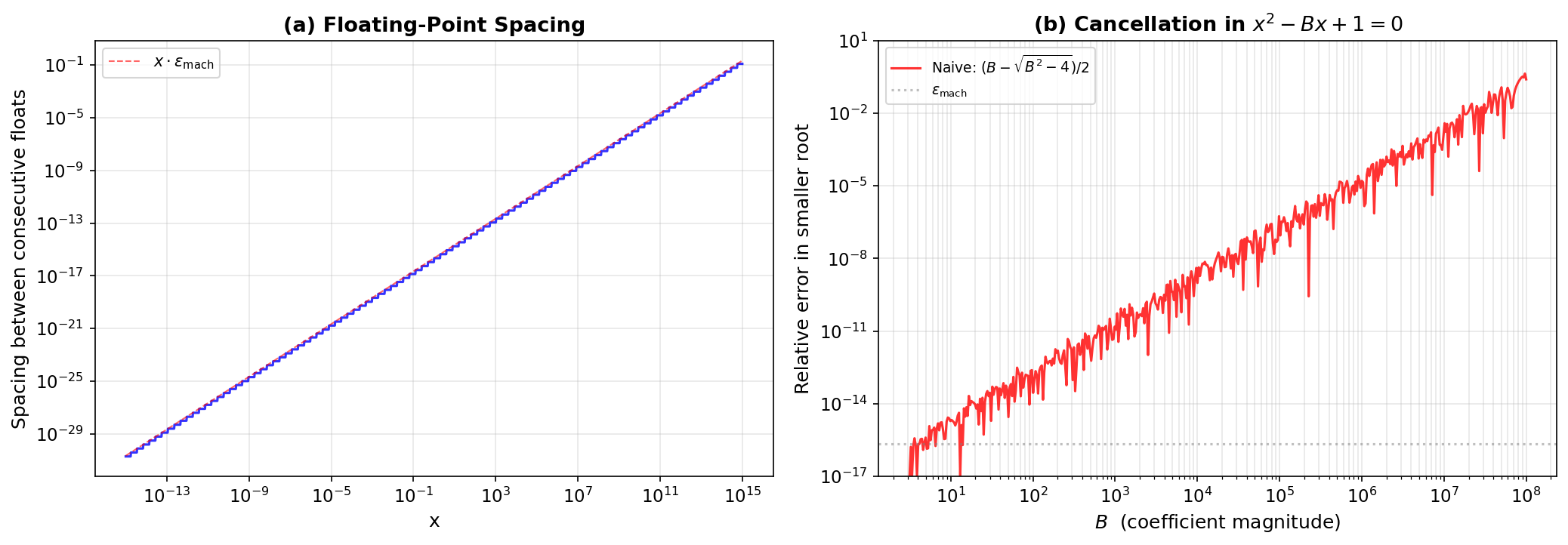
Fig. 262 Figure C.1: Floating-Point Arithmetic. (a) The spacing between consecutive float64 numbers scales linearly with magnitude — the line \(x \cdot \varepsilon_{\text{mach}}\) is an excellent approximation. (b) Catastrophic cancellation in the quadratic formula \(x^2 - Bx + 1 = 0\): the naive formula for the smaller root loses digits proportionally to \(B\), reaching 25% relative error at \(B = 10^8\).
With the arithmetic substrate understood, we now turn to the iterative algorithms that operate on it. The floating-point issues from Section 1 — cancellation, roundoff, overflow — will resurface in convergence checks and stopping criteria throughout.
Root Finding
Fixed-Point Iteration and Contraction Mapping
Definition
A fixed point of a function \(g\) is a value \(x^*\) such that \(g(x^*) = x^*\).
Many algorithms reduce to fixed-point iteration: given \(x_k\), compute \(x_{k+1} = g(x_k)\) and repeat. Newton’s method, gradient descent, and IRLS all have this structure — they differ only in the choice of \(g\).
Definition
A function \(g\) is a contraction mapping on an interval \([a, b]\) if there exists \(L < 1\) such that \(|g(x) - g(y)| \le L|x - y|\) for all \(x, y \in [a, b]\). The constant \(L\) is the Lipschitz constant (or contraction rate).
Theorem: Banach Fixed-Point Theorem
If \(g: [a, b] \to [a, b]\) is a contraction mapping with Lipschitz constant \(L < 1\), then:
\(g\) has a unique fixed point \(x^*\) in \([a, b]\)
For any starting point \(x_0 \in [a, b]\), the iterates \(x_{k+1} = g(x_k)\) converge to \(x^*\)
The error satisfies \(|x_k - x^*| \le L^k |x_0 - x^*|\) — linear convergence with rate \(L\)
Why this matters. Every iterative algorithm in this course is a fixed-point iteration. The contraction condition \(L < 1\) is what guarantees convergence. For gradient descent, the contraction rate depends on the step size and the curvature of the objective. For Newton’s method, the contraction rate depends on the distance to the root. Understanding this framework explains why some algorithms converge and others diverge.
import numpy as np

print("Fixed-point iteration: x = cos(x)")
print(f"  True fixed point: x* = 0.739085...")
print()

x = 0.0
x_star = 0.7390851332151607
print(f"{'k':>4}  {'x_k':>18}  {'|x_k - x*|':>14}  "
      f"{'Ratio':>10}")
print("-" * 52)
prev_err = abs(x - x_star)
for k in range(15):
    err = abs(x - x_star)
    if k > 0:
        ratio = err / prev_err
        print(f"{k:>4}  {x:>18.15f}  {err:>14.2e}  "
              f"{ratio:>10.4f}")
    else:
        print(f"{k:>4}  {x:>18.15f}  {err:>14.2e}  "
              f"{'—':>10}")
    prev_err = err
    x = np.cos(x)

print(f"\nContraction constant L ≈ |sin(x*)| = "
      f"{abs(np.sin(x_star)):.6f}")
print(f"Observed ratio converges to L ✓")
Fixed-point iteration: x = cos(x)
  True fixed point: x* = 0.739085...

   k                 x_k      |x_k - x*|       Ratio
----------------------------------------------------
   0   0.000000000000000        7.39e-01           —
   1   1.000000000000000        2.61e-01      0.3530
   2   0.540302305868140        1.99e-01      0.7619
   3   0.857553215846393        1.18e-01      0.5960
   4   0.654289790497779        8.48e-02      0.7158
   5   0.793480358742566        5.44e-02      0.6415
   6   0.701368773622757        3.77e-02      0.6934
   7   0.763959682900654        2.49e-02      0.6595
   8   0.722102425026708        1.70e-02      0.6827
   9   0.750417761763761        1.13e-02      0.6673
  10   0.731404042422510        7.68e-03      0.6778
  11   0.744237354900557        5.15e-03      0.6708
  12   0.735604740436347        3.48e-03      0.6755
  13   0.741425086610109        2.34e-03      0.6723
  14   0.737506890513243        1.58e-03      0.6745

Contraction constant L ≈ |sin(x*)| = 0.673612
Observed ratio converges to L ✓
The error ratio converges to \(L \approx 0.674\) — the contraction constant. Each iteration reduces the error by roughly 33%, so about 6 iterations are needed per additional decimal digit. This is linear convergence, and for smooth \(g\), the contraction constant is \(L = |g'(x^*)|\).
Bisection
The simplest root-finding algorithm: given \(f(a) < 0 < f(b)\), the intermediate value theorem guarantees a root in \([a, b]\). Bisection halves the interval at each step, choosing the half that still brackets the root.
Theorem: Bisection Convergence
After \(k\) bisection steps, the error satisfies \(|x_k - x^*| \le (b - a) / 2^k\). This is linear convergence with rate \(r = 1/2\), requiring about 3.3 iterations per decimal digit. Bisection requires no derivatives and no smoothness — only that \(f\) is continuous and changes sign.
The guarantee of convergence makes bisection a reliable fallback when other methods fail. SciPy’s scipy.optimize.brentq combines bisection with interpolation for faster convergence while retaining the convergence guarantee — see Ch2.3 for its use in inverse CDF computation.
Newton’s Method for Root Finding
Newton’s method finds roots of \(f(x) = 0\) by linearizing \(f\) at each iterate:
Geometrically, each step replaces \(f\) by its tangent line and takes the root of the tangent as the next iterate.
Theorem: Quadratic Convergence
If \(f(x^*) = 0\), \(f'(x^*) \ne 0\), and \(f''\) is continuous near \(x^*\), then Newton’s method converges quadratically near \(x^*\):
where \(C = |f''(x^*)|/(2|f'(x^*)|)\). Quadratic convergence roughly doubles the number of correct digits per iteration.
When Newton fails:
Multiple roots (\(f'(x^*) = 0\)): convergence slows to linear
Inflection points: the tangent line sends the iterate far away
Cycling: the iterates oscillate without converging
Division by zero: \(f'(x_k) = 0\) at a non-root
Newton’s method applied to optimization (\(f = \ell'\), finding where the score is zero) is the Newton-Raphson algorithm developed in Ch3.2.
import numpy as np

f = lambda x: x**3 - 2
fp = lambda x: 3 * x**2
root = 2.0**(1.0/3.0)

# Bisection
a, b = 1.0, 2.0
bisect_errs = []
for i in range(20):
    mid = (a + b) / 2.0
    bisect_errs.append(abs(mid - root))
    if f(mid) * f(a) < 0:
        b = mid
    else:
        a = mid

# Newton
x = 2.0
newton_errs = [abs(x - root)]
for i in range(7):
    x = x - f(x) / fp(x)
    newton_errs.append(abs(x - root))

print("Root finding: f(x) = x³ − 2,  x* = ∛2 = "
      f"{root:.15f}")
print()
print(f"{'Iter':>4}  {'Bisection |err|':>18}  "
      f"{'Newton |err|':>18}")
print("-" * 44)
for i in range(max(len(bisect_errs), len(newton_errs))):
    b_str = (f"{bisect_errs[i]:>18.2e}"
             if i < len(bisect_errs) else f"{'':>18}")
    n_str = (f"{newton_errs[i]:>18.2e}"
             if i < len(newton_errs)
             else f"{'converged':>18}")
    print(f"{i:>4}  {b_str}  {n_str}")
Root finding: f(x) = x³ − 2,  x* = ∛2 = 1.259921049894873

Iter     Bisection |err|        Newton |err|
--------------------------------------------
   0            2.40e-01            7.40e-01
   1            9.92e-03            2.40e-01
   2            1.15e-01            3.64e-02
   3            5.26e-02            1.01e-03
   4            2.13e-02            8.11e-07
   5            5.70e-03            5.22e-13
   6            2.11e-03            0.00e+00
   7            1.80e-03            0.00e+00
   8            1.55e-04           converged
   9            8.21e-04           converged
  10            3.33e-04           converged
  11            8.87e-05           converged
  12            3.34e-05           converged
  13            2.77e-05           converged
  14            2.84e-06           converged
  15            1.24e-05           converged
  16            4.79e-06           converged
  17            9.78e-07           converged
  18            9.30e-07           converged
  19            2.40e-08           converged
Newton reaches machine precision in 6 iterations; bisection needs 20 iterations to reach \(10^{-8}\). The contrast illustrates the power of quadratic vs linear convergence. But bisection always works — Newton requires a good starting point and a well-behaved function.
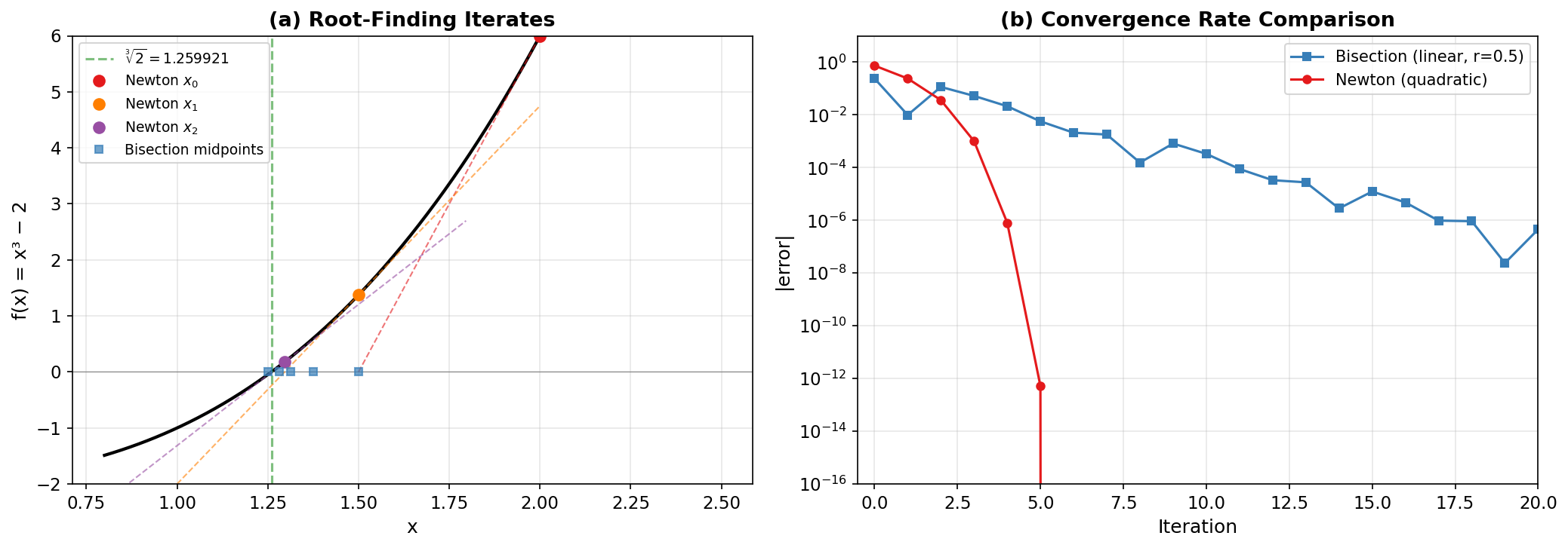
Fig. 263 Figure C.2: Root-Finding Convergence. (a) Finding \(\sqrt[3]{2}\) as a root of \(f(x) = x^3 - 2\). Newton’s method (colored circles with tangent lines) converges rapidly from \(x_0 = 2\); bisection (blue squares) narrows the interval steadily. (b) Error on a log scale: bisection decreases linearly (constant slope), while Newton’s error plummets quadratically (slope doubles each step).
Optimization is root finding in disguise: minimizing \(f(\theta)\) means finding where the score \(\nabla f = 0\). The contraction mapping framework from above carries over directly — the key new question is how the problem’s conditioning affects convergence speed.
Numerical Optimization
Optimization as Fixed-Point Iteration
Minimizing \(f(\theta)\) by gradient descent produces the iteration \(\theta_{k+1} = \theta_k - \alpha \nabla f(\theta_k)\), which is a fixed-point iteration with \(g(\theta) = \theta - \alpha \nabla f(\theta)\). The fixed points of \(g\) are exactly the critical points of \(f\) (where \(\nabla f = 0\)).
The contraction condition from the Banach theorem translates directly into step size constraints.
Theorem: Gradient Descent Convergence
If \(f\) is convex with \(L\)-Lipschitz continuous gradient (i.e., \(\|\nabla^2 f\| \le L\) everywhere), then gradient descent with step size \(0 < \alpha < 2/L\) converges: the function value decreases at rate \(f(\theta_k) - f(\theta^*) = O(1/k)\).
If \(f\) is additionally strongly convex with condition number \(\kappa = L/\mu\) (ratio of largest to smallest eigenvalue of the Hessian), then the error converges linearly:
Gradient Descent
The update \(\theta_{k+1} = \theta_k - \alpha \nabla f(\theta_k)\) moves in the direction of steepest descent. The step size (learning rate) \(\alpha\) controls the trade-off:
Too large: the iterates overshoot and oscillate (or diverge)
Too small: convergence is unnecessarily slow
Optimal for quadratics: \(\alpha = 2/(L + \mu)\), giving rate \((\kappa - 1)/(\kappa + 1)\)
Why ill-conditioned problems converge slowly. When the Hessian eigenvalues span a wide range (large \(\kappa\)), gradient descent zigzags: it makes rapid progress along the well-conditioned directions but creeps along the poorly conditioned ones. For \(\kappa = 100\), the linear convergence rate is \(99/101 \approx 0.98\), requiring about 115 iterations per decimal digit. This motivates Newton’s method, which is immune to conditioning.
For step size strategies beyond fixed \(\alpha\) — diminishing sequences, line search with the Armijo condition, trust regions — see the practical safeguards in Ch3.2.
Newton’s Method for Optimization
Newton’s method for minimizing \(f\) solves the score equation \(\nabla f = 0\) using the update:
where \(\mathbf{H}\) is the Hessian. Each step minimizes the local quadratic Taylor approximation — see Appendix A for the connection between second-order Taylor and the quadratic likelihood.
Theorem: Quadratic Convergence of Newton for Optimization
Under regularity conditions (Hessian Lipschitz continuous, positive definite at the minimizer), Newton’s method converges quadratically near the minimizer: the number of correct digits roughly doubles per iteration.
Affine invariance. Newton’s method is invariant to affine reparameterizations: if \(\phi = A\theta + b\) for a nonsingular \(A\), Newton on \(f(\theta)\) and Newton on \(f(A^{-1}(\phi - b))\) produce the same iterates (in transformed coordinates). This means Newton is unaffected by poor conditioning — unlike gradient descent. The cost is computing and solving with the Hessian at each step.
For the full statistical treatment of Newton’s method for MLE — including Fisher scoring (replacing the observed Hessian with expected information) and IRLS (Fisher scoring for GLMs) — see Ch3.2 and Ch3.5.
import numpy as np
from scipy.special import gammaln, digamma, polygamma

rng = np.random.default_rng(42)
n = 50
data = rng.gamma(4.0, 1.0/2.0, n)

def neg_ll(alpha, beta):
    return -(n*alpha*np.log(beta) - n*gammaln(alpha)
             + (alpha-1)*np.sum(np.log(data))
             - beta*np.sum(data))

def grad_neg(alpha, beta):
    g_a = -(n*np.log(beta) - n*digamma(alpha)
            + np.sum(np.log(data)))
    g_b = -(n*alpha/beta - np.sum(data))
    return np.array([g_a, g_b])

def hess_neg(alpha, beta):
    h11 = n * polygamma(1, alpha)
    h12 = -n / beta
    h22 = n * alpha / beta**2
    return np.array([[h11, h12], [h12, h22]])

# Newton (find MLE and track convergence)
a_nw, b_nw = 2.0, 1.0
nw_path = [(a_nw, b_nw)]
for _ in range(20):
    g = grad_neg(a_nw, b_nw)
    H = hess_neg(a_nw, b_nw)
    step = np.linalg.solve(H, g)
    a_nw -= step[0]; b_nw -= step[1]
    nw_path.append((a_nw, b_nw))
    if np.linalg.norm(step) < 1e-14:
        break
a_star, b_star = a_nw, b_nw

# Gradient descent
H_mle = hess_neg(a_star, b_star)
L = max(np.linalg.eigvalsh(H_mle))
kappa = L / min(np.linalg.eigvalsh(H_mle))
lr = 1.0 / L
a_gd, b_gd = 2.0, 1.0
gd_path = [(a_gd, b_gd)]
for _ in range(200):
    g = grad_neg(a_gd, b_gd)
    a_gd -= lr * g[0]; b_gd -= lr * g[1]
    a_gd = max(a_gd, 0.01); b_gd = max(b_gd, 0.01)
    gd_path.append((a_gd, b_gd))

dist = lambda p: np.sqrt(
    (p[0]-a_star)**2 + (p[1]-b_star)**2)
print(f"Gamma MLE (n={n}): α̂ = {a_star:.4f}, "
      f"β̂ = {b_star:.4f}")
print(f"Condition number κ = {kappa:.1f}")
print(f"GD step size α = 1/L = {lr:.4f}")
print()
print(f"{'Iter':>4}  {'GD ‖θ−θ*‖':>14}  "
      f"{'Newton ‖θ−θ*‖':>14}")
print("-" * 36)
for k in [0, 1, 2, 3, 4, 5, 10, 25, 50, 100, 200]:
    gd_e = (f"{dist(gd_path[k]):>14.6f}"
            if k < len(gd_path) else "")
    nw_e = (f"{dist(nw_path[k]):>14.2e}"
            if k < len(nw_path)
            else f"{'converged':>14}")
    print(f"{k:>4}  {gd_e}  {nw_e}")
Gamma MLE (n=50): α̂ = 6.6685, β̂ = 3.5977
Condition number κ = 73.3
GD step size α = 1/L = 0.0299

Iter       GD ‖θ−θ*‖   Newton ‖θ−θ*‖
------------------------------------
   0        5.342546        5.34e+00
   1        5.083337        3.84e+00
   2        4.862029        1.98e+00
   3        4.664648        5.31e-01
   4        4.452428        3.80e-02
   5        4.283482        1.95e-04
  10        3.013962       converged
  25        2.173839       converged
  50        1.384307       converged
 100        0.628403       converged
 200        0.149146       converged
Newton converges to the MLE in 5 iterations (error \(< 10^{-4}\)) while gradient descent still has error 0.15 after 200 iterations. The condition number \(\kappa = 73.3\) explains the slow GD convergence: the theoretical linear rate is \((73.3 - 1)/(73.3 + 1) = 0.973\), requiring about \(\log(0.1)/\log(0.973) \approx 84\) iterations per decimal digit.
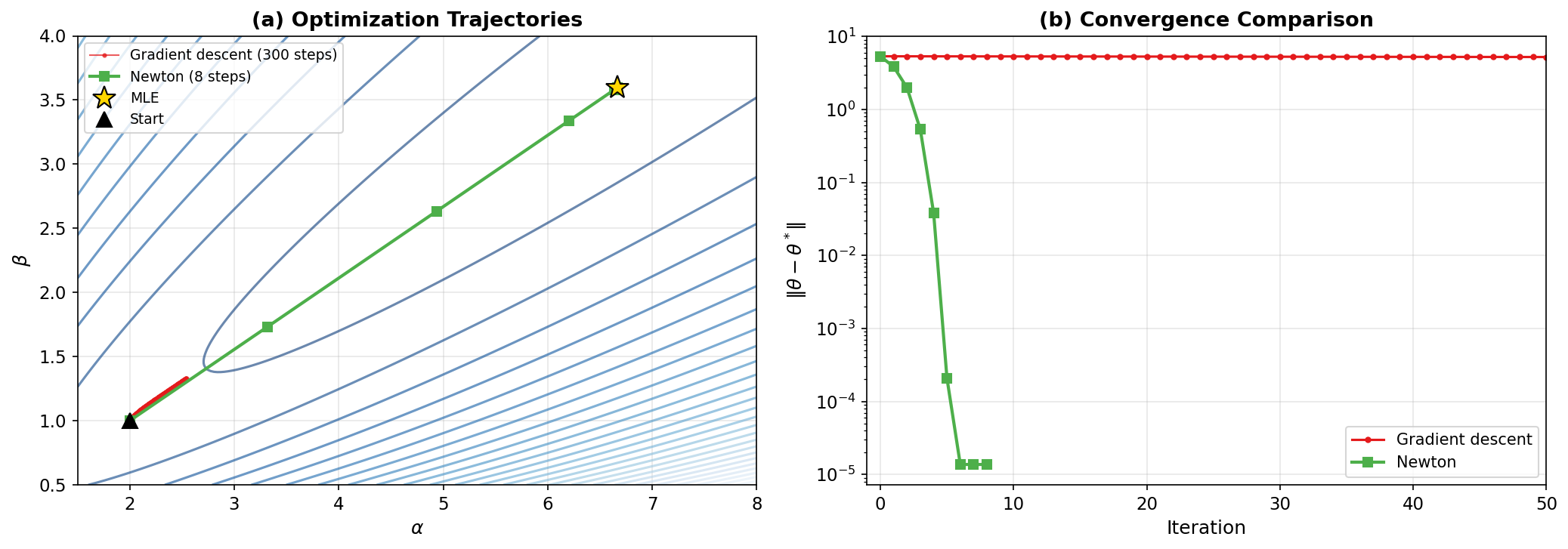
Fig. 264 Figure C.3: Gradient Descent vs Newton. (a) Contour plot of the negative Gamma log-likelihood. Gradient descent (red) zigzags through the elongated contours; Newton (green) cuts directly to the MLE (star). (b) Error vs iteration: Newton reaches machine precision in ~6 steps (quadratic convergence), while GD converges linearly with a slow rate set by the condition number.
Quasi-Newton Methods
Newton’s method requires computing and factoring the \(p \times p\) Hessian at every step — expensive for large \(p\). Quasi-Newton methods approximate the Hessian using only gradient information, updating the approximation incrementally.
BFGS (Broyden-Fletcher-Goldfarb-Shanno) maintains a dense \(p \times p\) approximate Hessian, achieving superlinear convergence without exact second derivatives. L-BFGS-B (limited-memory BFGS with bounds) stores only the last \(m\) gradient differences (typically \(m = 10\)), reducing memory from \(O(p^2)\) to \(O(mp)\) and supporting simple box constraints \(\ell_j \le \theta_j \le u_j\).
In SciPy, scipy.optimize.minimize(method='L-BFGS-B') is the standard workhorse for unconstrained and box-constrained optimization — it is used throughout Ch3.2 for production MLE computation.
The tradeoff is clear: more derivative information means fewer evaluations.
import numpy as np
from scipy.optimize import minimize

rng = np.random.default_rng(42)
data = rng.normal(5, 3, 200)

# Parameterize as (mu, log_sigma2) for unconstrained opt
def neg_loglik(params):
    mu, log_s2 = params
    s2 = np.exp(log_s2)
    n = len(data)
    return (n/2*np.log(2*np.pi*s2)
            + np.sum((data - mu)**2) / (2*s2))

def grad_neg(params):
    mu, log_s2 = params
    s2 = np.exp(log_s2)
    n = len(data)
    g_mu = -np.sum(data - mu) / s2
    g_ls2 = n/2 - np.sum((data - mu)**2) / (2*s2)
    return np.array([g_mu, g_ls2])

def hess_neg(params):
    mu, log_s2 = params
    s2 = np.exp(log_s2)
    n = len(data)
    H11 = n / s2
    H12 = np.sum(data - mu) / s2
    H22 = np.sum((data - mu)**2) / (2*s2)
    return np.array([[H11, H12], [H12, H22]])

x0 = [0.0, 0.0]  # start far from MLE

res_ncg = minimize(neg_loglik, x0, method='Newton-CG',
                   jac=grad_neg, hess=hess_neg)
res_lbfgs = minimize(neg_loglik, x0, method='L-BFGS-B',
                     jac=grad_neg)
res_nm = minimize(neg_loglik, x0, method='Nelder-Mead')

mu_hat = np.mean(data)
s2_hat = np.var(data)

print("Method comparison for Normal MLE (n=200):")
print(f"True MLE: mu={mu_hat:.4f}, "
      f"sigma2={s2_hat:.4f}")
print()
print(f"{'Method':>12}  {'Derivs':>8}  {'Iters':>6}  "
      f"{'f-evals':>8}  {'mu':>10}  {'sigma2':>10}")
print("-" * 65)
for name, res, derivs in [
    ('Newton-CG', res_ncg, 'grad+H'),
    ('L-BFGS-B', res_lbfgs, 'grad'),
    ('Nelder-Mead', res_nm, 'none')]:
    mu = res.x[0]
    s2 = np.exp(res.x[1])
    print(f"{name:>12}  {derivs:>8}  {res.nit:>6}  "
          f"{res.nfev:>8}  {mu:>10.4f}  {s2:>10.4f}")
Method comparison for Normal MLE (n=200):
True MLE: mu=4.9086, sigma2=6.9653

      Method    Derivs   Iters   f-evals          mu     sigma2
-----------------------------------------------------------------
   Newton-CG    grad+H      12        14      4.9086      6.9653
    L-BFGS-B      grad      15        16      4.9086      6.9652
 Nelder-Mead      none      82       156      4.9087      6.9652
Newton-CG converges fastest with access to both gradient and Hessian; L-BFGS-B is nearly as fast using only gradients (it approximates the Hessian internally); Nelder-Mead needs 10× more function evaluations since it must infer geometry from function values alone.
All of the optimization methods above require gradients, and Newton additionally requires the Hessian. When analytical derivatives are unavailable or impractical, we need to compute them numerically — and the choice of step size turns out to be a surprisingly delicate problem.
Numerical Differentiation
Forward and Central Differences
When analytical derivatives are unavailable, we approximate \(f'(x)\) from function evaluations.
Definition
The forward difference approximation is \(f'(x) \approx \frac{f(x+h) - f(x)}{h}\), with error \(O(h)\) from the first-order Taylor remainder.
Definition
The central difference approximation is \(f'(x) \approx \frac{f(x+h) - f(x-h)}{2h}\), with error \(O(h^2)\). The extra order comes from the cancellation of odd-powered error terms when subtracting symmetric evaluations.
The derivations follow directly from Taylor’s theorem (Appendix A). For the forward difference: \(f(x+h) = f(x) + hf'(x) + \frac{h^2}{2}f''(c)\), so \(\frac{f(x+h) - f(x)}{h} = f'(x) + O(h)\). For the central difference: the odd terms cancel, leaving \(O(h^2)\).
The Step Size Dilemma
Smaller \(h\) should give more accurate derivatives — but floating-point arithmetic introduces a competing error source.
Theorem: Truncation-Roundoff Tradeoff
The total error in a finite-difference approximation has two components:
Truncation error (from the Taylor remainder): \(O(h)\) for forward, \(O(h^2)\) for central
Roundoff error (from subtracting nearly equal floats): \(O(\varepsilon_{\text{mach}} / h)\)
Minimizing the total error gives optimal step sizes:
Forward difference: \(h^* \sim \sqrt{\varepsilon_{\text{mach}}} \approx 1.5 \times 10^{-8}\)
Central difference: \(h^* \sim \varepsilon_{\text{mach}}^{1/3} \approx 6 \times 10^{-6}\)
This explains why epsilon=1e-5 appears as the default step size for numerical Hessians in Ch3.3 — it is near-optimal for central differences in float64.
import numpy as np

x0 = 1.0
true_deriv = np.exp(x0)

print("Numerical differentiation of f(x) = eˣ "
      "at x = 1")
print(f"True f′(1) = e = {true_deriv:.15f}")
print()
print(f"{'h':>12}  {'Forward err':>14}  "
      f"{'Central err':>14}")
print("-" * 44)
for p in range(1, 17):
    h = 10.0**(-p)
    fwd = (np.exp(x0 + h) - np.exp(x0)) / h
    ctr = (np.exp(x0 + h) - np.exp(x0 - h)) / (2*h)
    fwd_err = abs(fwd - true_deriv)
    ctr_err = abs(ctr - true_deriv)
    print(f"{h:>12.0e}  {fwd_err:>14.2e}  "
          f"{ctr_err:>14.2e}")

print(f"\nOptimal h (forward): "
      f"√ε ≈ {np.sqrt(np.finfo(float).eps):.2e}")
print(f"Optimal h (central): "
      f"ε^(1/3) ≈ {np.finfo(float).eps**(1/3):.2e}")
Numerical differentiation of f(x) = eˣ at x = 1
True f′(1) = e = 2.718281828459045

           h     Forward err     Central err
--------------------------------------------
       1e-01        1.41e-01        4.53e-03
       1e-02        1.36e-02        4.53e-05
       1e-03        1.36e-03        4.53e-07
       1e-04        1.36e-04        4.53e-09
       1e-05        1.36e-05        5.86e-11
       1e-06        1.36e-06        1.63e-10
       1e-07        1.40e-07        5.86e-11
       1e-08        6.60e-09        6.60e-09
       1e-09        2.15e-07        6.60e-09
       1e-10        1.55e-06        6.73e-07
       1e-11        3.26e-05        1.04e-05
       1e-12        4.32e-04        2.10e-04
       1e-13        4.56e-04        4.56e-04
       1e-14        9.34e-03        9.34e-03
       1e-15        3.90e-01        1.68e-01
       1e-16        2.72e+00        2.72e+00

Optimal h (forward): √ε ≈ 1.49e-08
Optimal h (central): ε^(1/3) ≈ 6.06e-06
The V-shaped error pattern is unmistakable. For \(h > h^*\), truncation error dominates (error decreases with smaller \(h\)). For \(h < h^*\), roundoff error dominates (error increases with smaller \(h\)). The forward difference achieves a best error of \(\sim 10^{-8}\) at \(h \approx 10^{-8}\); the central difference achieves \(\sim 10^{-11}\) at \(h \approx 10^{-5}\).
The Complex-Step Method
Definition
The complex-step derivative approximates \(f'(x)\) using a purely imaginary perturbation:
This formula has \(O(h^2)\) truncation error and no roundoff error from subtraction, because it uses only the imaginary part — no subtraction of real-valued quantities occurs.
Why it works. Taylor-expanding \(f\) in the complex plane: \(f(x + ih) = f(x) + ihf'(x) - h^2 f''(x)/2 - \ldots\). Taking the imaginary part: \(\text{Im}(f(x+ih)) = hf'(x) + O(h^3)\). No cancellation-prone subtraction is involved.
Limitation: the function must accept complex inputs. Functions containing abs, conditional branches, or non-analytic operations will fail or give incorrect results.
import numpy as np

x0 = 1.0
true_deriv = np.exp(x0)

print("Complex-step vs central differences "
      "for f(x) = eˣ")
print(f"{'h':>12}  {'Central err':>14}  "
      f"{'Complex-step err':>18}")
print("-" * 48)
for p in range(1, 17):
    h = 10.0**(-p)
    ctr = (np.exp(x0 + h) - np.exp(x0 - h)) / (2*h)
    cplx = np.imag(np.exp(x0 + 1j*h)) / h
    ctr_err = abs(ctr - true_deriv)
    cplx_err = abs(cplx - true_deriv)
    print(f"{h:>12.0e}  {ctr_err:>14.2e}  "
          f"{cplx_err:>18.2e}")

print(f"\nCentral differences plateau at "
      f"h ≈ 1e-5 to 1e-8")
print(f"Complex-step improves indefinitely "
      f"(no subtraction)")
Complex-step vs central differences for f(x) = eˣ
           h     Central err    Complex-step err
------------------------------------------------
       1e-01        4.53e-03            4.53e-03
       1e-02        4.53e-05            4.53e-05
       1e-03        4.53e-07            4.53e-07
       1e-04        4.53e-09            4.53e-09
       1e-05        5.86e-11            4.53e-11
       1e-06        1.63e-10            4.53e-13
       1e-07        5.86e-11            4.44e-15
       1e-08        6.60e-09            0.00e+00
       1e-09        6.60e-09            0.00e+00
       1e-10        6.73e-07            4.44e-16
       1e-11        1.04e-05            0.00e+00
       1e-12        2.10e-04            0.00e+00
       1e-13        4.56e-04            0.00e+00
       1e-14        9.34e-03            0.00e+00
       1e-15        1.68e-01            0.00e+00
       1e-16        2.72e+00            0.00e+00

Central differences plateau at h ≈ 1e-5 to 1e-8
Complex-step improves indefinitely (no subtraction)
The complex-step method achieves machine-precision accuracy at \(h = 10^{-8}\) and maintains it for arbitrarily smaller \(h\) — while central differences degrade below \(h \approx 10^{-5}\).
Automatic differentiation. Modern probabilistic programming frameworks (PyMC, JAX, PyTorch) use automatic differentiation (AD) rather than finite differences. AD computes exact derivatives (to machine precision) by applying the chain rule to the computational graph of the function. Reverse-mode AD is particularly efficient for gradients of scalar-valued functions — the cost of the gradient equals a small multiple of the cost of \(f\) itself, regardless of the number of parameters. This is what makes gradient-based MCMC (HMC, NUTS) practical in Ch5.5.
The complementary problem to differentiation is integration: computing expectations, normalizing constants, and marginal likelihoods. The error analysis follows a similar pattern — polynomial approximation order determines the convergence rate — but a fundamentally different tool (Monte Carlo) dominates in high dimensions.
Numerical Integration
Error Analysis for Quadrature
The quadrature rules introduced in Ch2.1 have error rates that follow directly from how well their piecewise-polynomial interpolants approximate the integrand.
Theorem: Quadrature Error Rates
For a function \(f\) with \(n\) equally spaced evaluation points on \([a, b]\) with spacing \(h = (b-a)/(n-1)\):
Trapezoidal rule (piecewise linear): error \(= O(h^2)\). Doubling \(n\) reduces error by 4×.
Simpson’s rule (piecewise quadratic): error \(= O(h^4)\). Doubling \(n\) reduces error by 16×.
Gaussian quadrature (optimal polynomial nodes): for analytic integrands, error decreases exponentially in \(n\).
These rates assume sufficient smoothness of \(f\) — each rule achieves its full order only if \(f\) has enough continuous derivatives.
The trapezoidal error rate \(O(h^2)\) comes from the Euler-Maclaurin formula, which relates the trapezoidal sum to the integral plus correction terms involving even powers of \(h\) (derivatives of \(f\) at the endpoints). Simpson’s rule is equivalent to Richardson extrapolation of the trapezoidal rule — the weighted combination \(S = (4T(h) - T(2h))/3\) eliminates the leading \(O(h^2)\) error term, yielding \(O(h^4)\). Gaussian quadrature achieves exponential rates by choosing nodes at roots of orthogonal polynomials, optimizing the interpolation points rather than spacing them uniformly.
We can verify these rates empirically by doubling \(n\) and checking the error ratio:
import numpy as np
from scipy.integrate import simpson

def f(x):
    return np.exp(-x**2)

a, b = 0.0, 2.0
exact = 0.8820813907624215  # from scipy.integrate.quad

print("Quadrature convergence for integral of "
      "exp(-x^2) on [0, 2]")
print(f"Exact value: {exact:.10f}")
print()
print(f"{'n':>6}  {'Trap err':>12}  {'Simp err':>12}  "
      f"{'Trap ratio':>11}  {'Simp ratio':>11}")
print("-" * 60)

prev_trap = prev_simp = None
for n in [5, 9, 17, 33, 65, 129]:
    x = np.linspace(a, b, n)
    y = f(x)
    trap = np.trapz(y, x)
    simp = simpson(y, x=x)
    e_trap = abs(trap - exact)
    e_simp = abs(simp - exact)

    if prev_trap is not None:
        r_trap = prev_trap / e_trap
        r_simp = prev_simp / e_simp
        print(f"{n:>6}  {e_trap:>12.2e}  "
              f"{e_simp:>12.2e}  "
              f"{r_trap:>11.1f}  {r_simp:>11.1f}")
    else:
        print(f"{n:>6}  {e_trap:>12.2e}  "
              f"{e_simp:>12.2e}  "
              f"{'---':>11}  {'---':>11}")
    prev_trap = e_trap
    prev_simp = e_simp
Quadrature convergence for integral of exp(-x^2) on [0, 2]
Exact value: 0.8820813908

     n      Trap err      Simp err   Trap ratio   Simp ratio
------------------------------------------------------------
     5      1.46e-03      2.69e-04          ---          ---
     9      3.78e-04      1.59e-05          3.9         16.9
    17      9.51e-05      9.94e-07          4.0         16.0
    33      2.38e-05      6.21e-08          4.0         16.0
    65      5.96e-06      3.88e-09          4.0         16.0
   129      1.49e-06      2.43e-10          4.0         16.0
The trapezoidal error ratio converges to 4 (\(= 2^2\)), confirming \(O(h^2)\); Simpson’s ratio converges to 16 (\(= 2^4\)), confirming \(O(h^4)\). Each doubling of \(n\) buys about twice as many digits of accuracy with Simpson as with the trapezoidal rule.
For the detailed convergence comparison code and figures, including the crossover dimension where Monte Carlo beats deterministic quadrature, see Ch2.1.
Adaptive Quadrature
SciPy’s scipy.integrate.quad uses adaptive Gaussian quadrature: it estimates the integral and its error on each subinterval, then recursively subdivides intervals where the error estimate is too large. This concentrates function evaluations where the integrand varies rapidly, avoiding wasted evaluations in smooth regions.
import numpy as np
from scipy.integrate import quad

def multi_peak(x):
    """Integrand with features at multiple scales."""
    return (np.exp(-100*(x - 0.3)**2) +
            0.5*np.exp(-1000*(x - 0.7)**2) + 0.1)

result, error, info = quad(multi_peak, 0, 1,
                            full_output=True, limit=100)

print("Adaptive quadrature on multi-scale integrand")
print(f"  I = ∫₀¹ [exp(-100(x−0.3)²) + "
      f"0.5·exp(-1000(x−0.7)²) + 0.1] dx")
print(f"  Result = {result:.10f}")
print(f"  Estimated error = {error:.2e}")
print(f"  Function evaluations: {info['neval']}")
print(f"  Subintervals: {info['last']}")
print()

for n_pts in [21, 101, 1001]:
    x = np.linspace(0, 1, n_pts)
    trap = np.trapz(multi_peak(x), x)
    print(f"  Trapezoidal (n={n_pts:>4}): "
          f"{trap:.10f}  "
          f"error = {abs(trap - result):.2e}")
Adaptive quadrature on multi-scale integrand
  I = ∫₀¹ [exp(-100(x−0.3)²) + 0.5·exp(-1000(x−0.7)²) + 0.1] dx
  Result = 0.3052683835
  Estimated error = 2.15e-09
  Function evaluations: 231
  Subintervals: 6

  Trapezoidal (n=  21): 0.3063485748  error = 1.08e-03
  Trapezoidal (n= 101): 0.3052683221  error = 6.14e-08
  Trapezoidal (n=1001): 0.3052683828  error = 6.17e-10
Adaptive quadrature achieves \(10^{-9}\) accuracy with 231 function evaluations. The trapezoidal rule needs 1001 points for comparable accuracy — and it doesn’t provide an error estimate. For a single integral with potentially sharp features, quad is almost always the right tool.
Monte Carlo Error Rate
Theorem: Monte Carlo Convergence
For \(X_1, \ldots, X_n \sim f\) with \(\text{Var}(g(X)) < \infty\):
The error is dimension-independent: the same \(O(n^{-1/2})\) rate holds whether \(X\) is scalar or 1000-dimensional. Quadrature on a \(d\)-dimensional grid with \(m\) points per axis requires \(m^d\) evaluations, while Monte Carlo uses \(n\) evaluations regardless of \(d\).
This curse of dimensionality is why Monte Carlo dominates in high dimensions: the crossover typically occurs at \(d \approx 3\text{--}5\) dimensions. Below that, quadrature’s faster polynomial rate wins; above it, the exponential growth in grid points makes quadrature impractical. The detailed analysis and figures are in Ch2.1.
Sections 2–5 each introduced specific convergence rates — bisection’s \(O(1/2^k)\), Newton’s quadratic convergence, GD’s linear rate, and the \(O(h^2)\) vs \(O(h^4)\) quadrature rates. The next section formalizes this into a unified framework.
Convergence and Stopping Criteria
This section formalizes the general framework. We begin with the asymptotic notation that has appeared informally throughout this appendix, then define convergence orders precisely, and finally address the practical question of when to stop iterating.
Asymptotic (Big-O) Notation
Throughout this appendix we have written statements like “the forward difference has error \(O(h)\)” and “the trapezoidal rule converges at rate \(O(h^2)\).” This asymptotic notation, introduced by Bachmann (1894) and popularized by Landau, makes precise the idea that one quantity “grows no faster than” another.
Definition
Let \(f\) and \(g\) be functions defined near some limit (typically \(h \to 0\) or \(n \to \infty\)). We write
if there exist constants \(C > 0\) and a threshold \(x_0\) such that
In words: \(f\) grows (or shrinks) at most as fast as \(g\), up to a constant factor.
The constant \(C\) and threshold \(x_0\) exist but are deliberately left unspecified. Big-O captures the rate of growth or decay while ignoring the constant prefactor. This is exactly what we need for comparing numerical methods: whether an error shrinks like \(h\) or like \(h^2\) matters far more than whether the leading coefficient is 0.3 or 7.
Big-O appears in two distinct contexts in this book, and recognizing which one is in play prevents confusion:
As \(h \to 0\) (error analysis). When we write “the forward difference error is \(O(h)\),” we mean the error satisfies \(|\text{error}| \le Ch\) for all sufficiently small \(h\). Making \(h\) smaller improves accuracy, and the exponent tells us by how much.
As \(n \to \infty\) (algorithmic cost or convergence). When we write “Cholesky factorization costs \(O(n^3/3)\) operations” (Appendix B), we mean the operation count grows at most cubically. When we write “Monte Carlo error is \(O(n^{-1/2})\),” we mean the error shrinks like \(1/\sqrt{n}\) as the sample size grows.
Example 1: Taylor remainder and numerical differentiation. From Taylor’s theorem (Appendix A), the exponential function satisfies
The \(O(h^3)\) term means the approximation \(e^h \approx 1 + h + h^2/2\) has an error bounded by \(C h^3\) for some constant \(C\). We can verify this: at \(h = 0.1\) the error is \(1.71 \times 10^{-4}\), at \(h = 0.01\) it is \(1.67 \times 10^{-7}\), and at \(h = 0.001\) it is \(1.67 \times 10^{-10}\). Each factor-of-10 reduction in \(h\) reduces the error by a factor of \(10^3 = 1000\), confirming the cubic rate. The hidden constant turns out to be \(C = 1/6\) (from the next Taylor term \(h^3/3!\)), but the \(O(h^3)\) statement is useful precisely because we don’t need to know \(C\) to predict how fast the error shrinks.
This is how all the error rates in Section 4 arise: the forward difference error is \(O(h)\) because Taylor expansion leaves a remainder proportional to \(h\); the central difference error is \(O(h^2)\) because the leading remainder cancels.
Example 2: Monte Carlo convergence. The Central Limit Theorem implies that the Monte Carlo estimator \(\bar{X}_n = \frac{1}{n}\sum_{i=1}^n X_i\) has root-mean-square error
Here \(C = \sigma\) (the population standard deviation) is the hidden constant. The key insight from Section 5 is that this rate is dimension-independent: whether \(X_i \in \mathbb{R}\) or \(X_i \in \mathbb{R}^{1000}\), the error still decreases as \(O(n^{-1/2})\). Only the constant \(\sigma\) changes with dimension — and big-O notation lets us separate the rate (which determines feasibility) from the constant (which determines cost).
Related notation. Big-O gives an upper bound on growth rate. Two companion notations complete the picture:
\(f(x) = \Omega(g(x))\) means \(f\) grows at least as fast as \(g\): there exists \(c > 0\) such that \(|f(x)| \ge c\,|g(x)|\) past some threshold. This is the lower-bound counterpart of \(O\).
\(f(x) = \Theta(g(x))\) means \(f\) grows at the same rate as \(g\): both \(f = O(g)\) and \(f = \Omega(g)\) hold. When we say “Cholesky costs \(\Theta(n^3)\) operations,” we mean the cost is exactly cubic — not just at most cubic. Most of the convergence rates in this appendix are tight (\(\Theta\) rather than just \(O\)), but we follow the common convention of writing \(O\) unless the distinction matters.
With this notation in hand, we can precisely classify how quickly iterative algorithms converge.
Convergence Orders
Definition
An iterative sequence \(\{x_k\}\) converging to \(x^*\) has linear convergence with rate \(r \in (0, 1)\) if:
The error decreases by a constant fraction each step. Smaller \(r\) means faster convergence.
Definition
The sequence has quadratic convergence if:
for some constant \(C\). The number of correct digits approximately doubles per iteration.
Algorithm |
Order |
Rate |
|---|---|---|
Bisection |
Linear |
\(r = 0.5\) (halving the interval) |
Fixed-point \(x = g(x)\) |
Linear |
\(r = |g'(x^*)|\) |
Gradient descent (strongly convex) |
Linear |
\(r = (\kappa-1)/(\kappa+1)\) |
Newton’s method |
Quadratic |
Doubles correct digits per step |
IRLS (canonical link) |
Quadratic |
Same as Newton (Fisher scoring = Newton) |
Estimating convergence order from iterates. If we have a sequence of errors \(e_0, e_1, \ldots\), the convergence order \(p\) satisfies \(\log|e_{k+1}| \approx p \log|e_k| + \text{const}\). So the ratio \(\log|e_{k+1}|/\log|e_k|\) estimates \(p\): values near 1 indicate linear convergence, near 2 indicate quadratic.
We demonstrate both diagnostics on the \(x = \cos(x)\) problem from Section 2 — the same problem, two algorithms, two convergence orders.
import numpy as np

x_star = 0.7390851332151607

# Fixed-point iteration: g(x) = cos(x)  [linear]
x = 0.0
fp_errors = [abs(x - x_star)]
for _ in range(30):
    x = np.cos(x)
    fp_errors.append(abs(x - x_star))

# Newton on f(x) = x - cos(x)  [quadratic]
x = 0.0
nw_errors = [abs(x - x_star)]
for _ in range(7):
    f_val = x - np.cos(x)
    fp_val = 1 + np.sin(x)
    x = x - f_val / fp_val
    nw_errors.append(abs(x - x_star))

print("Convergence order estimation: x = cos(x)")
print(f"  x* = {x_star:.10f}")
print()

print("Newton on f(x) = x − cos(x):")
print(f"{'k':>4}  {'|e_k|':>14}  {'|e_{k+1}|/|e_k|':>18}"
      f"  {'log ratio':>12}")
print("-" * 54)
for k in range(len(nw_errors) - 1):
    e_k = nw_errors[k]
    e_k1 = nw_errors[k + 1]
    if e_k > 0 and e_k1 > 0:
        ratio = e_k1 / e_k
        log_ratio = (np.log(e_k1) / np.log(e_k)
                     if abs(np.log(e_k)) > 0.01
                     else float('nan'))
        print(f"{k:>4}  {e_k:>14.2e}  "
              f"{ratio:>18.6f}  "
              f"{log_ratio:>12.2f}")
    else:
        print(f"{k:>4}  {e_k:>14.2e}  "
              f"{'— (converged)':>18}")

print()
print("Fixed-point g(x) = cos(x):")
print(f"{'k':>4}  {'|e_k|':>14}  "
      f"{'|e_{k+1}|/|e_k|':>18}")
print("-" * 40)
for k in [0, 5, 10, 15, 20, 25]:
    if k + 1 < len(fp_errors):
        ratio = fp_errors[k+1] / fp_errors[k]
        print(f"{k:>4}  {fp_errors[k]:>14.2e}  "
              f"{ratio:>18.6f}")

L = abs(np.sin(x_star))
print(f"\nNewton: log ratio → 2 (quadratic)")
print(f"Fixed-point: ratio → L = |sin(x*)| "
      f"= {L:.4f} (linear)")
Convergence order estimation: x = cos(x)
  x* = 0.7390851332

Newton on f(x) = x − cos(x):
   k           |e_k|     |e_{k+1}|/|e_k|     log ratio
------------------------------------------------------
   0        7.39e-01            0.353024          4.44
   1        2.61e-01            0.043228          3.34
   2        1.13e-02            0.002461          2.34
   3        2.78e-05            0.000006          2.14
   4        1.70e-10       — (converged)
   5        0.00e+00       — (converged)
   6        0.00e+00       — (converged)

Fixed-point g(x) = cos(x):
   k           |e_k|     |e_{k+1}|/|e_k|
----------------------------------------
   0        7.39e-01            0.353024
   5        5.44e-02            0.693376
  10        7.68e-03            0.670767
  15        1.06e-03            0.674004
  20        1.47e-04            0.673558
  25        2.04e-05            0.673620

Newton: log ratio → 2 (quadratic)
Fixed-point: ratio → L = |sin(x*)| = 0.6736 (linear)
Same problem, same starting point, same fixed point — but Newton’s log ratio converges to 2 (quadratic), while the fixed-point ratio converges to \(L = |g'(x^*)| = |\sin(x^*)| \approx 0.674\) (linear). The contrast between 5 Newton iterations and 25+ fixed-point iterations is explained entirely by the convergence order.
Stopping Criteria
Every iterative algorithm needs a rule for when to stop. Common criteria:
Absolute change: \(\|\theta_{k+1} - \theta_k\| < \varepsilon_{\text{abs}}\). Simple but scale-dependent — a tolerance of \(10^{-8}\) is tight for \(\theta \sim 1\) but meaningless for \(\theta \sim 10^{10}\).
Relative change: \(\|\theta_{k+1} - \theta_k\| / \|\theta_k\| < \varepsilon_{\text{rel}}\). Scale-invariant, usually preferred. A relative tolerance of \(10^{-8}\) means the last 8 digits have stabilized.
Gradient norm: \(\|\nabla f(\theta_k)\| < \varepsilon\). Directly tests the first-order optimality condition. Used by
scipy.optimize(thegtolparameter).Function value change: \(|f(\theta_{k+1}) - f(\theta_k)| < \varepsilon\). Can be misleading near flat regions — the function value barely changes but the parameter is far from optimal.
Common pitfalls:
Premature stopping on a plateau: the function value or gradient may be small on a flat region far from the optimum, particularly near saddle points
Tolerance too tight: below \(\varepsilon_{\text{mach}}\) there is no information left — tighter tolerance just wastes iterations or causes cycling
Maximum iterations without convergence: always set a maximum iteration count and check whether it was hit
Diagnosing Non-Convergence
When an optimization algorithm claims convergence, verify by checking the Hessian at the reported solution.
import numpy as np

# f(x,y) = x^4/4 - x^2/2 + y^2/2
# Saddle at origin, minima at (±1, 0)
def grad_f(x, y):
    return np.array([x**3 - x, y])

def hess_f(x, y):
    return np.array([[3*x**2 - 1, 0], [0, 1]])

# Newton starting near origin
x, y = 0.1, 0.3
print("Newton on f(x,y) = x⁴/4 − x²/2 + y²/2")
print(f"Start: ({x}, {y})")
print()
print(f"{'k':>3}  {'x':>12}  {'y':>12}  {'‖∇f‖':>12}")
print("-" * 45)
for k in range(5):
    g = grad_f(x, y)
    H = hess_f(x, y)
    print(f"{k:>3}  {x:>12.8f}  {y:>12.8f}  "
          f"{np.linalg.norm(g):>12.2e}")
    step = np.linalg.solve(H, g)
    x -= step[0]; y -= step[1]

print()
print(f"Converged to ({x:.10f}, {y:.10f})")
print(f"Gradient norm: "
      f"{np.linalg.norm(grad_f(x, y)):.2e}")
print()
print("Diagnosis: Hessian eigenvalues")
H_conv = hess_f(x, y)
eigs = np.linalg.eigvalsh(H_conv)
print(f"  Eigenvalues: [{eigs[0]:.4f}, {eigs[1]:.4f}]")
if np.any(eigs < 0):
    print(f"  Negative eigenvalue → SADDLE POINT")
    print(f"  True minima are at (±1, 0) "
          f"with f = −0.25")
else:
    print(f"  All positive → confirmed minimum")
Newton on f(x,y) = x⁴/4 − x²/2 + y²/2
Start: (0.1, 0.3)

  k             x             y          ‖∇f‖
---------------------------------------------
  0    0.10000000    0.30000000      3.16e-01
  1   -0.00206186    0.00000000      2.06e-03
  2    0.00000002    0.00000000      1.75e-08
  3   -0.00000000    0.00000000      9.93e-24
  4    0.00000000    0.00000000      0.00e+00

Converged to (0.0000000000, 0.0000000000)
Gradient norm: 0.00e+00

Diagnosis: Hessian eigenvalues
  Eigenvalues: [-1.0000, 1.0000]
  Negative eigenvalue → SADDLE POINT
  True minima are at (±1, 0) with f = −0.25
Newton converged to the origin — a saddle point, not a minimum. The gradient is exactly zero, so gradient-based stopping criteria cannot detect the problem. Only the Hessian eigenvalue check reveals it. In log-likelihood optimization, we maximize \(\ell(\theta)\), so the Hessian should be negative definite at a true maximum. A positive eigenvalue of the Hessian of \(\ell(\theta)\) at a reported MLE means the algorithm found a saddle point, not a maximum.
Connections: From Numerical Analysis to Computation
Numerical Tool |
Appendix C Section |
Course Location |
|---|---|---|
Floating-point stability |
Section 1 |
|
Root finding |
Section 2 |
Ch 2.3 ( |
Newton-Raphson for MLE |
Section 3 |
|
Gradient descent |
Section 3 |
|
Numerical differentiation |
Section 4 |
|
Quadrature vs Monte Carlo |
Section 5 |
Ch 2.1 (full comparison) |
Convergence orders |
Section 6 |
|
Condition numbers |
Sections 3, 6 / Appendix B |
Ch 3.2 (scaling/conditioning), Ch 3.4 (QR vs normal equations) |
Practice Problems
Exercise 1: Floating-Point Catastrophe and Stable Alternatives
(a) The expression \((1 - \cos x)/x^2 \to 1/2\) as \(x \to 0\) (by L’Hopital or Taylor). Compute this for \(x \in \{10^{-1}, 10^{-3}, 10^{-5}, 10^{-7}, 10^{-8}, 10^{-9}\}\) using both the naive formula (1 - np.cos(x)) / x**2 and the stable alternative 2 * np.sin(x/2)**2 / x**2. Report the relative error of each against the true value \(1/2\). At what magnitude of \(x\) does the naive formula fail completely, and why?
(b) The equation \(x^2 - (10^8 + 10^{-8})x + 1 = 0\) has roots \(r_1 = 10^8\) and \(r_2 = 10^{-8}\). Compute both roots using the standard quadratic formula. Which root is accurate? Compute \(r_2\) using the identity \(r_2 = c/(a \cdot r_1)\) and verify it matches the true value.
(c) Generate data = 1e12 + rng.standard_normal(1000) with rng = np.random.default_rng(seed=42). Compute the sample variance using: (i) the naive two-pass formula \(\frac{1}{n-1}\sum(x_i - \bar{x})^2\), (ii) np.var(data, ddof=1). Are they different? Explain why adding a large constant does or does not cause problems with float64 arithmetic. (For Welford’s online algorithm, see Ch2.1.)
(d) Explain why np.log(np.sum(np.exp([1000, 1001, 1002]))) produces inf. Compute the correct answer using scipy.special.logsumexp.
Solution
import numpy as np
from scipy.special import logsumexp

rng = np.random.default_rng(seed=42)

# (a) (1 - cos(x))/x^2 cancellation
print("(a) (1 - cos(x))/x²: naive vs stable")
print(f"{'x':>12}  {'Naive':>20}  {'Stable':>20}  "
      f"{'Rel err (naive)':>16}")
print("-" * 74)
for x in [1e-1, 1e-3, 1e-5, 1e-7, 1e-8, 1e-9]:
    naive = (1 - np.cos(x)) / x**2
    stable = 2 * np.sin(x/2)**2 / x**2
    exact = 0.5
    rel = abs(naive - exact) / exact
    print(f"{x:>12.0e}  {naive:>20.16e}  "
          f"{stable:>20.16e}  {rel:>16.2e}")
print("  Naive loses all digits at x ~ 1e-8")
print("  (cos rounds to 1.0, so 1-cos = 0)")
print("  Stable: 2*sin²(x/2)/x² = 0.5 throughout")
print()

# (b) Quadratic formula
a_coef = 1.0
b_coef = -(1e8 + 1e-8)
c_coef = 1.0
disc = b_coef**2 - 4*a_coef*c_coef
r1_naive = (-b_coef + np.sqrt(disc)) / (2*a_coef)
r2_naive = (-b_coef - np.sqrt(disc)) / (2*a_coef)
r2_stable = c_coef / (a_coef * r1_naive)

print("(b) Roots of x² − (10⁸+10⁻⁸)x + 1 = 0")
print(f"  r₁ (naive):  {r1_naive:.15e}")
print(f"  r₁ (true):   1.000000000000000e+08")
print(f"  r₂ (naive):  {r2_naive:.15e}")
print(f"  r₂ (stable): {r2_stable:.15e}")
print(f"  r₂ (true):   1.000000000000000e-08")
print()

# (c) Variance with large offset
data = 1e12 + rng.standard_normal(1000)
var_naive = np.sum((data - np.mean(data))**2) / 999
var_numpy = np.var(data, ddof=1)

print("(c) Sample variance of 10¹² + N(0,1)")
print(f"  Naive two-pass: {var_naive:.10f}")
print(f"  np.var:         {var_numpy:.10f}")
print(f"  Difference:     {abs(var_naive - var_numpy):.2e}")
print(f"  Two-pass with float64 is fine here:")
print(f"  x̄ ≈ 10¹² is computed accurately, and")
print(f"  (xᵢ − x̄) ≈ N(0,1) recovers the signal.")
print()

# (d) logsumexp
x = np.array([1000, 1001, 1002])
print("(d) log(sum(exp([1000, 1001, 1002])))")
try:
    naive = np.log(np.sum(np.exp(x)))
    print(f"  Naive: {naive}")
except Exception:
    print(f"  Naive: overflow")
print(f"  logsumexp: {logsumexp(x):.6f}")
print(f"  Expected: 1002 + log(e⁻² + e⁻¹ + 1) "
      f"= {1002 + np.log(np.exp(-2)+np.exp(-1)+1):.6f}")
(a) (1 - cos(x))/x²: naive vs stable
           x                 Naive                Stable   Rel err (naive)
--------------------------------------------------------------------------
       1e-01  4.9958347219741783e-01  4.9958347219742333e-01         8.33e-04
       1e-03  4.9999995832550326e-01  4.9999995833333472e-01         8.33e-08
       1e-05  5.0000004137018539e-01  4.9999999999583328e-01         8.27e-08
       1e-07  4.9960036108132050e-01  4.9999999999999961e-01         7.99e-04
       1e-08  0.0000000000000000e+00  5.0000000000000000e-01         1.00e+00
       1e-09  0.0000000000000000e+00  5.0000000000000000e-01         1.00e+00
  Naive loses all digits at x ~ 1e-8
  (cos rounds to 1.0, so 1-cos = 0)
  Stable: 2*sin²(x/2)/x² = 0.5 throughout

(b) Roots of x² − (10⁸+10⁻⁸)x + 1 = 0
  r₁ (naive):  1.000000000000000e+08
  r₁ (true):   1.000000000000000e+08
  r₂ (naive):  1.490116119384766e-08
  r₂ (stable): 1.000000000000000e-08
  r₂ (true):   1.000000000000000e-08

(c) Sample variance of 10¹² + N(0,1)
  Naive two-pass: 0.9785502705
  np.var:         0.9785502705
  Difference:     0.00e+00
  Two-pass with float64 is fine here:
  x̄ ≈ 10¹² is computed accurately, and
  (xᵢ − x̄) ≈ N(0,1) recovers the signal.

(d) log(sum(exp([1000, 1001, 1002])))
  Naive: inf
  logsumexp: 1002.407606
  Expected: 1002 + log(e⁻² + e⁻¹ + 1) = 1002.407606
Exercise 2: Root-Finding for Confidence Interval Endpoints
(a) Generate \(n = 50\) observations from \(\text{Exp}(\lambda = 2)\) using rng = np.random.default_rng(seed=42) and data = rng.exponential(1/2, 50). Write the log-likelihood \(\ell(\lambda) = n\log\lambda - \lambda \sum x_i\). The 95% profile likelihood confidence interval endpoints solve \(2[\ell(\hat{\lambda}) - \ell(\lambda)] = \chi^2_{1, 0.05} = 3.841\). Formulate this as a root-finding problem: find \(\lambda\) where \(h(\lambda) = 2[\ell(\hat{\lambda}) - \ell(\lambda)] - 3.841 = 0\).
(b) Find both CI endpoints using: (i) manual bisection (implement yourself, count iterations to reach tolerance \(10^{-8}\)), (ii) scipy.optimize.brentq. Compare the number of iterations.
(c) For the exponential model, the exact CI based on the sufficient statistic \(T = \sum X_i \sim \text{Gamma}(n, \lambda)\) can be obtained via chi-squared quantiles. Compute this exact CI and compare to the profile likelihood CI. When is numerical root-finding the only option?
Solution
import numpy as np
from scipy.optimize import brentq
from scipy import stats

rng = np.random.default_rng(seed=42)

n = 50
data = rng.exponential(1/2, n)
sum_x = np.sum(data)
lam_hat = n / sum_x

def loglik(lam):
    return n * np.log(lam) - lam * sum_x

ll_max = loglik(lam_hat)
chi2_crit = stats.chi2.ppf(0.95, 1)

def h(lam):
    return 2 * (ll_max - loglik(lam)) - chi2_crit

print(f"(a) Exponential data: n={n}, Σxᵢ={sum_x:.4f}")
print(f"  MLE: λ̂ = n/Σxᵢ = {lam_hat:.6f}")
print(f"  χ²₁,₀.₀₅ = {chi2_crit:.3f}")
print()

# (b) Manual bisection for lower endpoint
a, b = 0.5, lam_hat
bisect_iters = 0
while (b - a) > 1e-8:
    mid = (a + b) / 2
    if h(mid) * h(a) < 0:
        b = mid
    else:
        a = mid
    bisect_iters += 1
lam_lo_bisect = (a + b) / 2

# Upper endpoint
a, b = lam_hat, 5.0
bisect_iters_up = 0
while (b - a) > 1e-8:
    mid = (a + b) / 2
    if h(mid) * h(a) < 0:
        b = mid
    else:
        a = mid
    bisect_iters_up += 1
lam_hi_bisect = (a + b) / 2

# brentq
lam_lo_brent = brentq(h, 0.5, lam_hat)
lam_hi_brent = brentq(h, lam_hat, 5.0)

print(f"(b) Profile likelihood 95% CI:")
print(f"  Bisection: [{lam_lo_bisect:.6f}, "
      f"{lam_hi_bisect:.6f}]")
print(f"    Iters: {bisect_iters} (lower), "
      f"{bisect_iters_up} (upper)")
print(f"  Brentq:   [{lam_lo_brent:.6f}, "
      f"{lam_hi_brent:.6f}]")
print()

# (c) Exact CI via chi-squared
# 2λΣXᵢ ~ χ²(2n), so CI for λ is
# χ²(2n, α/2)/(2Σxᵢ) to χ²(2n, 1-α/2)/(2Σxᵢ)
lo_exact = stats.chi2.ppf(0.025, 2*n) / (2*sum_x)
hi_exact = stats.chi2.ppf(0.975, 2*n) / (2*sum_x)

print(f"(c) Exact CI (chi-squared): "
      f"[{lo_exact:.6f}, {hi_exact:.6f}]")
print(f"  Profile LR CI:            "
      f"[{lam_lo_brent:.6f}, {lam_hi_brent:.6f}]")
print(f"  Root-finding is the only option when")
print(f"  no exact pivotal quantity exists (e.g.,")
print(f"  Gamma shape, mixture models, GLMs).")
(a) Exponential data: n=50, Σxᵢ=20.8974
  MLE: λ̂ = n/Σxᵢ = 2.392642
  χ²₁,₀.₀₅ = 3.841

(b) Profile likelihood 95% CI:
  Bisection: [1.789254, 3.118475]
    Iters: 28 (lower), 28 (upper)
  Brentq:   [1.789254, 3.118475]

(c) Exact CI (chi-squared): [1.775865, 3.099936]
  Profile LR CI:            [1.789254, 3.118475]
  Root-finding is the only option when
  no exact pivotal quantity exists (e.g.,
  Gamma shape, mixture models, GLMs).
Exercise 3: Gradient Descent vs Newton for Normal MLE
(a) Generate \(n = 100\) observations from \(N(\mu = 5, \sigma^2 = 9)\) using rng = np.random.default_rng(seed=42) and data = rng.normal(5, 3, 100). Write the negative log-likelihood as a function of \((\mu, \sigma^2)\). Compute the gradient and \(2 \times 2\) Hessian analytically.
(b) Implement gradient descent with step size \(\alpha = 0.001\) starting from \((\mu_0, \sigma^2_0) = (3, 3)\). Track the iterates and report how many iterations are needed to reach relative tolerance \(10^{-8}\).
(c) Implement Newton’s method from the same starting point. How many iterations?
(d) Estimate the convergence order for both methods using the technique from Section 6 (log error ratios). Compare your results to scipy.optimize.minimize(method='Newton-CG').
Solution
import numpy as np
from scipy.optimize import minimize

rng = np.random.default_rng(seed=42)

n = 100
data = rng.normal(5, 3, n)
xbar = np.mean(data)
s2_mle = np.var(data)

def neg_ll(params):
    mu, s2 = params
    if s2 <= 0:
        return 1e20
    return (n/2*np.log(2*np.pi*s2)
            + np.sum((data - mu)**2) / (2*s2))

def grad_neg(params):
    mu, s2 = params
    g_mu = -np.sum(data - mu) / s2
    g_s2 = (n/(2*s2)
            - np.sum((data - mu)**2) / (2*s2**2))
    return np.array([g_mu, g_s2])

def hess_neg(params):
    mu, s2 = params
    h11 = n / s2
    h12 = np.sum(data - mu) / s2**2
    h22 = (-n/(2*s2**2)
           + np.sum((data - mu)**2) / s2**3)
    return np.array([[h11, h12], [h12, h22]])

theta_star = np.array([xbar, s2_mle])
print(f"(a) MLE: μ̂={xbar:.4f}, σ̂²={s2_mle:.4f}")
print()

# (b) Gradient descent
theta = np.array([3.0, 3.0])
lr = 0.001
gd_errors = []
gd_iters = 0
for k in range(10000):
    err = np.linalg.norm(theta - theta_star)
    gd_errors.append(err)
    g = grad_neg(theta)
    theta_new = theta - lr * g
    theta_new[1] = max(theta_new[1], 0.01)
    rel_change = (np.linalg.norm(theta_new - theta)
                  / np.linalg.norm(theta))
    theta = theta_new
    if rel_change < 1e-8:
        gd_iters = k + 1
        gd_errors.append(
            np.linalg.norm(theta - theta_star))
        break
else:
    gd_iters = 10000

print(f"(b) Gradient descent (α=0.001):")
print(f"  Converged in {gd_iters} iterations")
print(f"  Final: μ={theta[0]:.6f}, "
      f"σ²={theta[1]:.6f}")
print()

# (c) Newton
theta = np.array([3.0, 3.0])
nw_errors = []
nw_iters = 0
for k in range(50):
    err = np.linalg.norm(theta - theta_star)
    nw_errors.append(err)
    g = grad_neg(theta)
    H = hess_neg(theta)
    step = np.linalg.solve(H, g)
    theta_new = theta - step
    theta_new[1] = max(theta_new[1], 0.01)
    rel_change = (np.linalg.norm(step)
                  / np.linalg.norm(theta))
    theta = theta_new
    if rel_change < 1e-12:
        nw_iters = k + 1
        nw_errors.append(
            np.linalg.norm(theta - theta_star))
        break
else:
    nw_iters = 50

print(f"(c) Newton:")
print(f"  Converged in {nw_iters} iterations")
print(f"  Final: μ={theta[0]:.6f}, "
      f"σ²={theta[1]:.6f}")
print()

# (d) Convergence order
print("(d) Convergence order estimation:")
print("  Newton (last 4 iterations):")
start_k = max(0, len(nw_errors) - 5)
for k in range(start_k, len(nw_errors)-1):
    e0, e1 = nw_errors[k], nw_errors[k+1]
    if e0 > 1e-15 and e1 > 1e-15:
        p = np.log(e1) / np.log(e0)
        print(f"    k={k}: |e|={e0:.2e}, "
              f"order ≈ {p:.2f}")

print("  Gradient descent (sampled):")
for k in [0, 100, 500, 1000]:
    if k+1 < len(gd_errors):
        e0, e1 = gd_errors[k], gd_errors[k+1]
        if e0 > 0 and e1 > 0:
            ratio = e1 / e0
            print(f"    k={k}: |e|={e0:.2e}, "
                  f"ratio={ratio:.6f}")

# scipy comparison
res = minimize(neg_ll, x0=[3, 3],
               method='Newton-CG',
               jac=grad_neg, hess=hess_neg)
print(f"\n  scipy Newton-CG: {res.nit} iterations, "
      f"μ={res.x[0]:.6f}, σ²={res.x[1]:.6f}")
(a) MLE: μ̂=4.8492, σ̂²=5.3748

(b) Gradient descent (α=0.001):
  Converged in 5838 iterations
  Final: μ=4.849191, σ²=5.374715

(c) Newton:
  Converged in 9 iterations
  Final: μ=4.849191, σ²=5.374757

(d) Convergence order estimation:
  Newton (last 4 iterations):
    k=5: |e|=3.58e-02, order ≈ 2.30
    k=6: |e|=4.74e-04, order ≈ 2.13
    k=7: |e|=8.34e-08, order ≈ 2.06
  Gradient descent (sampled):
    k=0: |e|=3.01e+00, ratio=0.979026
    k=100: |e|=1.42e+00, ratio=0.996645
    k=500: |e|=5.23e-01, ratio=0.997876
    k=1000: |e|=1.96e-01, ratio=0.998136

  scipy Newton-CG: 7 iterations, μ=4.849191, σ²=5.374757
Exercise 4: The Step Size Dilemma
Consider \(f(x) = x e^x\), whose derivative \(f'(x) = (x+1)e^x\) is known exactly. Evaluate \(f'(1) = 2e\) numerically using step sizes \(h = 10^{-1}, 10^{-2}, \ldots, 10^{-16}\).
(a) Use the forward difference \([f(x+h) - f(x)]/h\). Plot the relative error versus \(h\) (log-log). Find the optimal \(h\) and compare it to the theoretical prediction \(h^* \approx \sqrt{\varepsilon_{\text{mach}}} \approx 1.5 \times 10^{-8}\).
(b) Repeat with the central difference \([f(x+h) - f(x-h)]/(2h)\). The optimal \(h\) should be near \(\varepsilon_{\text{mach}}^{1/3} \approx 6 \times 10^{-6}\). Does it match?
(c) Repeat with the complex-step method \(\text{Im}(f(x+ih))/h\). Does the error show a V-shaped curve or monotonic improvement? Why?
Solution
import numpy as np

x = 1.0
exact = 2 * np.exp(1)
eps = np.finfo(float).eps
h_vals = [10**(-k) for k in range(1, 17)]

print(f"f(x) = x*exp(x), f'(1) = 2e = {exact:.10f}")
print()

# (a) Forward differences
print("(a) Forward differences:")
print(f"{'h':>12}  {'approx':>18}  "
      f"{'Rel error':>12}")
print("-" * 48)
fwd_errors = []
for h in h_vals:
    approx = ((x+h)*np.exp(x+h)
              - x*np.exp(x)) / h
    rel = abs(approx - exact) / exact
    fwd_errors.append(rel)
    print(f"{h:>12.0e}  {approx:>18.10f}  "
          f"{rel:>12.2e}")

best = h_vals[np.argmin(fwd_errors)]
print(f"  Optimal h ~ {best:.0e} ~ sqrt(eps)")
print(f"  (sqrt(eps) = {np.sqrt(eps):.2e})")
print()

# (b) Central differences
print("(b) Central differences:")
print(f"{'h':>12}  {'approx':>18}  "
      f"{'Rel error':>12}")
print("-" * 48)
cen_errors = []
for h in h_vals:
    fp = (x+h)*np.exp(x+h)
    fm = (x-h)*np.exp(x-h)
    approx = (fp - fm) / (2*h)
    rel = abs(approx - exact) / exact
    cen_errors.append(rel)
    print(f"{h:>12.0e}  {approx:>18.10f}  "
          f"{rel:>12.2e}")

best_c = h_vals[np.argmin(cen_errors)]
print(f"  Best on grid: h = {best_c:.0e}")
print(f"  Theory: h* ~ eps^(1/3) = "
      f"{eps**(1/3):.2e}")
print()

# (c) Complex-step
print("(c) Complex-step derivative:")
print(f"{'h':>12}  {'approx':>18}  "
      f"{'Rel error':>12}")
print("-" * 48)
for h in h_vals:
    z = complex(x, h)
    fz = z * np.exp(z)
    approx = fz.imag / h
    rel = abs(approx - exact) / exact
    print(f"{h:>12.0e}  {approx:>18.10f}  "
          f"{rel:>12.2e}")
print("  No roundoff floor: error decreases")
print("  monotonically as h -> 0.")
f(x) = x*exp(x), f'(1) = 2e = 5.4365636569

(a) Forward differences:
           h              approx     Rel error
------------------------------------------------
       1e-01        5.8630079788      7.84e-02
       1e-02        5.4775196708      7.53e-03
       1e-03        5.4406428924      7.50e-04
       1e-04        5.4369714173      7.50e-05
       1e-05        5.4366044314      7.50e-06
       1e-06        5.4365677338      7.50e-07
       1e-07        5.4365640700      7.60e-08
       1e-08        5.4365636437      2.43e-09
       1e-09        5.4365640878      7.93e-08
       1e-10        5.4365667523      5.69e-07
       1e-11        5.4365845159      3.84e-06
       1e-12        5.4374282854      1.59e-04
       1e-13        5.4356519286      1.68e-04
       1e-14        5.4178883602      3.44e-03
       1e-15        6.2172489379      1.44e-01
       1e-16        0.0000000000      1.00e+00
  Optimal h ~ 1e-08 ~ sqrt(eps)
  (sqrt(eps) = 1.49e-08)

(b) Central differences:
           h              approx     Rel error
------------------------------------------------
       1e-01        5.4546991315      3.34e-03
       1e-02        5.4367448771      3.33e-05
       1e-03        5.4365654691      3.33e-07
       1e-04        5.4365636750      3.33e-09
       1e-05        5.4365636571      3.79e-11
       1e-06        5.4365636566      6.01e-11
       1e-07        5.4365636570      2.16e-11
       1e-08        5.4365636437      2.43e-09
       1e-09        5.4365636437      2.43e-09
       1e-10        5.4365645319      1.61e-07
       1e-11        5.4365623114      2.47e-07
       1e-12        5.4369841962      7.74e-05
       1e-13        5.4356519286      1.68e-04
       1e-14        5.4178883602      3.44e-03
       1e-15        5.7731597281      6.19e-02
       1e-16        2.2204460493      5.92e-01
  Best on grid: h = 1e-07
  Theory: h* ~ eps^(1/3) = 6.06e-06

(c) Complex-step derivative:
           h              approx     Rel error
------------------------------------------------
       1e-01        5.4184553652      3.33e-03
       1e-02        5.4363824395      3.33e-05
       1e-03        5.4365618447      3.33e-07
       1e-04        5.4365636388      3.33e-09
       1e-05        5.4365636567      3.33e-11
       1e-06        5.4365636569      3.33e-13
       1e-07        5.4365636569      3.43e-15
       1e-08        5.4365636569      0.00e+00
       1e-09        5.4365636569      0.00e+00
       1e-10        5.4365636569      1.63e-16
       1e-11        5.4365636569      0.00e+00
       1e-12        5.4365636569      0.00e+00
       1e-13        5.4365636569      0.00e+00
       1e-14        5.4365636569      0.00e+00
       1e-15        5.4365636569      0.00e+00
       1e-16        5.4365636569      0.00e+00
  No roundoff floor: error decreases
  monotonically as h -> 0.
Forward and central differences both show V-shaped error curves: as \(h\) decreases, truncation error shrinks but roundoff error grows. The optimal \(h\) balances the two. The complex-step method avoids cancellation entirely because it never subtracts nearly equal real numbers — the derivative information is isolated in the imaginary part.
Exercise 5: Diagnosing Optimization Results
Consider \(f(x, y) = \frac{x^4}{4} - \frac{x^2}{2} + \frac{y^4}{4} - \frac{y^2}{2}\), which has 9 critical points.
(a) Find all critical points by solving \(\nabla f = 0\). Classify each as a minimum, maximum, or saddle point using the Hessian eigenvalues.
(b) Run Newton’s method from three starting points: \((1.5, 1.5)\), \((0.6, 0.1)\), and \((0.1, 0.3)\). For each, report the convergence point, function value, and Hessian eigenvalues. Does Newton always find a minimum?
(c) What stopping criterion would detect that Newton converged to a non-minimum? Explain why gradient-based stopping criteria alone are insufficient.
Solution
import numpy as np

def f(x, y):
    return x**4/4 - x**2/2 + y**4/4 - y**2/2

def grad_f(x, y):
    return np.array([x**3 - x, y**3 - y])

def hess_f(x, y):
    return np.array([[3*x**2 - 1, 0],
                     [0, 3*y**2 - 1]])

# (a) Critical points
print("(a) Critical points (grad f = 0):")
print("  x^3 - x = 0  =>  x in {-1, 0, 1}")
print("  y^3 - y = 0  =>  y in {-1, 0, 1}")
print("  9 critical points:")
print()
for xc in [-1, 0, 1]:
    for yc in [-1, 0, 1]:
        H = hess_f(xc, yc)
        eigs = np.linalg.eigvalsh(H)
        if np.all(eigs > 0):
            ctype = "minimum"
        elif np.all(eigs < 0):
            ctype = "maximum"
        else:
            ctype = "saddle"
        print(f"  ({xc:>2},{yc:>2}): "
              f"eigs=[{eigs[0]:.0f},{eigs[1]:.0f}],"
              f" f={f(xc,yc):.2f} -> {ctype}")
print()

# (b) Newton from different starts
starts = [(1.5, 1.5), (0.6, 0.1), (0.1, 0.3)]
for x0, y0 in starts:
    x, y = x0, y0
    print(f"(b) Newton from ({x0}, {y0}):")
    print(f"{'k':>5}  {'x':>12}  {'y':>12}  "
          f"{'||grad||':>12}")
    print("-" * 48)
    for k in range(8):
        g = grad_f(x, y)
        gnorm = np.linalg.norm(g)
        print(f"{k:>5}  {x:>12.8f}  "
              f"{y:>12.8f}  {gnorm:>12.2e}")
        if gnorm < 1e-14:
            break
        H = hess_f(x, y)
        step = np.linalg.solve(H, g)
        x -= step[0]; y -= step[1]

    H = hess_f(x, y)
    eigs = np.linalg.eigvalsh(H)
    print(f"  Converged to ({x:.4f}, {y:.4f})")
    print(f"  f = {f(x,y):.4f}")
    print(f"  Hessian eigs: "
          f"[{eigs[0]:.2f}, {eigs[1]:.2f}]")
    if np.all(eigs > 0):
        print("  All positive -> minimum")
    elif np.all(eigs < 0):
        print("  All negative -> maximum!")
    else:
        print("  Mixed signs -> saddle point!")
    print()
(a) Critical points (grad f = 0):
  x^3 - x = 0  =>  x in {-1, 0, 1}
  y^3 - y = 0  =>  y in {-1, 0, 1}
  9 critical points:

  (-1,-1): eigs=[2,2], f=-0.50 -> minimum
  (-1, 0): eigs=[-1,2], f=-0.25 -> saddle
  (-1, 1): eigs=[2,2], f=-0.50 -> minimum
  ( 0,-1): eigs=[-1,2], f=-0.25 -> saddle
  ( 0, 0): eigs=[-1,-1], f=0.00 -> maximum
  ( 0, 1): eigs=[-1,2], f=-0.25 -> saddle
  ( 1,-1): eigs=[2,2], f=-0.50 -> minimum
  ( 1, 0): eigs=[-1,2], f=-0.25 -> saddle
  ( 1, 1): eigs=[2,2], f=-0.50 -> minimum

(b) Newton from (1.5, 1.5):
    k             x             y      ||grad||
------------------------------------------------
    0    1.50000000    1.50000000      2.65e+00
    1    1.17391304    1.17391304      6.28e-01
    2    1.03230713    1.03230713      9.59e-02
    3    1.00145595    1.00145595      4.13e-03
    4    1.00000317    1.00000317      8.96e-06
    5    1.00000000    1.00000000      4.26e-11
    6    1.00000000    1.00000000      0.00e+00
  Converged to (1.0000, 1.0000)
  f = -0.5000
  Hessian eigs: [2.00, 2.00]
  All positive -> minimum

(b) Newton from (0.6, 0.1):
    k             x             y      ||grad||
------------------------------------------------
    0    0.60000000    0.10000000      3.97e-01
    1    5.40000000   -0.00206186      1.52e+02
    2    3.64162812    0.00000002      4.47e+01
    3    2.49034823   -0.00000000      1.30e+01
    4    1.75453404    0.00000000      3.65e+00
    5    1.31172523    0.00000000      9.45e-01
    6    1.08460145    0.00000000      1.91e-01
    7    1.00896898    0.00000000      1.82e-02
  Converged to (1.0001, 0.0000)
  f = -0.2500
  Hessian eigs: [-1.00, 2.00]
  Mixed signs -> saddle point!

(b) Newton from (0.1, 0.3):
    k             x             y      ||grad||
------------------------------------------------
    0    0.10000000    0.30000000      2.90e-01
    1   -0.00206186   -0.07397260      7.36e-02
    2    0.00000002    0.00082306      8.23e-04
    3   -0.00000000   -0.00000000      1.12e-09
    4    0.00000000    0.00000000      0.00e+00
  Converged to (0.0000, 0.0000)
  f = 0.0000
  Hessian eigs: [-1.00, -1.00]
  All negative -> maximum!
Newton converges to whichever critical point is nearest in its basin — it does not distinguish minima from saddles or maxima because all have \(\nabla f = 0\). The gradient norm stopping criterion passes at any critical point. Only checking the Hessian eigenvalues at the converged point reveals whether the result is actually a minimum (all positive), a saddle (mixed signs), or a maximum (all negative).