Section 4.5: Jackknife Methods

The bootstrap, introduced by Efron in 1979, revolutionized computational statistics by providing a general-purpose tool for uncertainty quantification. But the bootstrap had an important predecessor: the jackknife, developed by Quenouille (1949) for bias reduction and extended by Tukey (1958) for variance estimation. While the bootstrap has largely superseded the jackknife for interval construction, the jackknife remains valuable in its own right—it is deterministic, computationally efficient for smooth statistics, and provides unique diagnostic capabilities through its connection to influence functions.

This section develops the jackknife as both a historical precursor to the bootstrap and a modern tool with distinct strengths. We begin with the delete-1 jackknife, extend to the delete-$d$ generalization, explore bias correction, and conclude with a systematic comparison to bootstrap methods. Throughout, we emphasize when each method excels and how they can be used together.

Road Map 🧭

Understand: The jackknife principle as systematic leave-one-out perturbation analysis
Develop: Computational skills for jackknife standard errors, bias estimation, and diagnostics
Implement: Delete-1 and delete-$d$ jackknife algorithms in Python
Evaluate: When to prefer jackknife over bootstrap, and when to use both

Historical Context and Motivation

The jackknife emerged from a practical problem: how to assess the reliability of a complex statistic without deriving its theoretical variance. Maurice Quenouille introduced the method in 1949 for bias reduction in serial correlation estimation, and John Tukey named it the “jackknife” in 1958, likening it to a versatile pocket knife that can help in many situations.

The Historical Problem

Consider estimating a parameter $\theta = T(F)$ with a statistic $\hat{\theta} = T(\hat{F}_n)$. For many statistics beyond the sample mean, deriving $\text{Var}(\hat{\theta})$ analytically requires either:

Strong distributional assumptions (e.g., normality)
Taylor expansions (delta method) that may be complex
Asymptotic approximations that may be inaccurate for small $n$

The jackknife provides an empirical alternative: by systematically observing how $\hat{\theta}$ changes when each observation is removed, we can approximate both the variance and bias of $\hat{\theta}$ without any distributional assumptions.

The Core Insight

For a smooth statistic $T$, removing a single observation $X_i$ from the sample approximates a small perturbation to the empirical distribution $\hat{F}_n$. If $T$ is sufficiently regular (differentiable in an appropriate sense), the change $\hat{\theta}_{(-i)} - \hat{\theta}$ reflects the influence of observation $X_i$ on the estimate. Aggregating these influences across all observations recovers information about the sampling variability of $\hat{\theta}$.

This is precisely the intuition behind the influence function from robust statistics, and we will see that the jackknife provides a discrete approximation to influence-function-based variance estimation.

The Delete-1 Jackknife

The delete-1 (or leave-one-out) jackknife is the foundation of jackknife methodology. We systematically compute the statistic on each of the $n$ subsamples formed by removing one observation.

Notation and Basic Definitions

Let $X_1, \ldots, X_n$ be an iid sample from distribution $F$, and let $\hat{\theta} = T(X_1, \ldots, X_n)$ be a statistic estimating $\theta = T(F)$.

Leave-one-out estimate: For each $i = 1, \ldots, n$, define

\[\hat{\theta}_{(-i)} = T(X_1, \ldots, X_{i-1}, X_{i+1}, \ldots, X_n)\]

This is the statistic computed on the sample with observation $X_i$ removed.

Jackknife average: The mean of the leave-one-out estimates is

\[\bar{\theta}_{(\cdot)} = \frac{1}{n} \sum_{i=1}^n \hat{\theta}_{(-i)}\]

Pseudovalues: Tukey introduced the pseudovalues

\[\widetilde{\theta}_i = n\hat{\theta} - (n-1)\hat{\theta}_{(-i)}\]

These act like $n$ “replicates” of the original estimate. Their sample mean equals the bias-corrected jackknife estimate:

\[\frac{1}{n} \sum_{i=1}^n \widetilde{\theta}_i = n\hat{\theta} - (n-1)\bar{\theta}_{(\cdot)} = \hat{\theta}^{\text{jack-bc}}\]

This equals $\hat{\theta}$ only when $\bar{\theta}_{(\cdot)} = \hat{\theta}$ (i.e., when the statistic is approximately unbiased or linear in the observations). For biased statistics, the mean of pseudovalues provides a bias-corrected estimate.

Intuition for Pseudovalues

Think of each pseudovalue $\widetilde{\theta}_i$ as answering: “What would $\hat{\theta}$ have been if observation $X_i$ had $n$ times its actual weight?” The pseudovalues inflate the influence of each observation, making the variability due to individual observations explicit.

Jackknife Standard Error

The jackknife standard error is computed from the variability of the leave-one-out estimates:

\[\widehat{\text{SE}}_{\text{jack}} = \sqrt{\frac{n-1}{n} \sum_{i=1}^n \left(\hat{\theta}_{(-i)} - \bar{\theta}_{(\cdot)}\right)^2}\]

The factor $(n-1)/n$ (rather than $1/n$) accounts for the fact that leave-one-out estimates are computed on samples of size $n-1$, not $n$. This scaling ensures correct variance estimation for smooth statistics.

Equivalently, the jackknife SE can be expressed using pseudovalues:

\[\widehat{\text{SE}}_{\text{jack}} = \frac{1}{\sqrt{n}} \cdot s_{\widetilde{\theta}}\]

where $s_{\widetilde{\theta}}$ is the sample standard deviation of the pseudovalues $\widetilde{\theta}_1, \ldots, \widetilde{\theta}_n$ (using divisor $n-1$).

For vector statistics $\hat{\boldsymbol{\theta}} \in \mathbb{R}^p$, the jackknife covariance matrix is:

\[\widehat{\text{Cov}}_{\text{jack}}(\hat{\boldsymbol{\theta}}) = \frac{n-1}{n} \sum_{i=1}^n \left(\hat{\boldsymbol{\theta}}_{(-i)} - \bar{\boldsymbol{\theta}}_{(\cdot)}\right)\left(\hat{\boldsymbol{\theta}}_{(-i)} - \bar{\boldsymbol{\theta}}_{(\cdot)}\right)^\top\]

Marginal standard errors are the square roots of diagonal elements, and the standard error of a linear combination $\mathbf{a}^\top\hat{\boldsymbol{\theta}}$ is $\sqrt{\mathbf{a}^\top \widehat{\text{Cov}}_{\text{jack}} \, \mathbf{a}}$.

Why the Jackknife Works

For statistics that are smooth functionals of $F$, the jackknife SE is consistent. The key theoretical result connects the jackknife to the influence function.

Influence Function: For a functional $T$ and distribution $F$, the influence function is

\[\text{IF}(x; T, F) = \lim_{\epsilon \to 0} \frac{T((1-\epsilon)F + \epsilon \delta_x) - T(F)}{\epsilon}\]

where $\delta_x$ is a point mass at $x$. This measures the rate of change of $T$ when we contaminate $F$ with a small mass at $x$.

Connection to Jackknife: For smooth statistics, the jackknife residuals approximate the empirical influence function. Removing observation $i$ changes the empirical distribution from $\hat{F}_n$ (uniform weights $1/n$) to $\hat{F}_{n,-i}$ (uniform weights $1/(n-1)$ on remaining observations). The scaled jackknife difference

\[(n-1)(\hat{\theta} - \hat{\theta}_{(-i)}) \approx \text{IF}(X_i; T, \hat{F}_n)\]

approximates the empirical influence function evaluated at each observation. The factor $(n-1)$ rather than $n$ arises because the leave-one-out empirical distribution has weights $1/(n-1)$.

Asymptotic Variance: Under regularity conditions, the asymptotic variance of $\sqrt{n}(\hat{\theta} - \theta)$ is

\[\sigma^2 = \int \text{IF}(x; T, F)^2 \, dF(x)\]

The jackknife variance estimator consistently estimates this quantity:

\[n \cdot \widehat{\text{SE}}_{\text{jack}}^2 \xrightarrow{p} \sigma^2\]

This explains why the jackknife works for smooth statistics—it approximates the influence-function variance formula.

Python Implementation

import numpy as np

def jackknife_se(data, statistic):
    """
    Compute the jackknife standard error of a statistic.

    Parameters
    ----------
    data : array_like
        Original data (1D array or 2D with observations along axis 0).
    statistic : callable
        Function that computes the statistic from data. May return
        a scalar or array.

    Returns
    -------
    se_jack : float or ndarray
        Jackknife standard error (same shape as statistic output).
    theta_hat : float or ndarray
        Original estimate from full data.
    theta_i : ndarray
        Leave-one-out estimates, shape (n,) or (n, p) for vector statistics.
    """
    data = np.asarray(data)
    n = len(data)

    # Compute original estimate and determine shape
    theta_hat = np.asarray(statistic(data))

    # Allocate array for leave-one-out estimates (handles scalar or vector)
    theta_i = np.empty((n,) + theta_hat.shape, dtype=float)

    for i in range(n):
        # Remove observation i
        if data.ndim == 1:
            data_minus_i = np.delete(data, i)
        else:
            data_minus_i = np.delete(data, i, axis=0)
        theta_i[i] = statistic(data_minus_i)

    # Jackknife SE formula (works for scalar or vector)
    theta_bar = theta_i.mean(axis=0)
    se_jack = np.sqrt(((n - 1) / n) * np.sum((theta_i - theta_bar)**2, axis=0))

    return se_jack, theta_hat, theta_i


def jackknife_pseudovalues(theta_hat, theta_i):
    """
    Compute jackknife pseudovalues.

    Parameters
    ----------
    theta_hat : float
        Original estimate from full data.
    theta_i : array_like
        Leave-one-out estimates.

    Returns
    -------
    pv : ndarray
        Pseudovalues.
    """
    theta_i = np.asarray(theta_i)
    n = len(theta_i)
    pv = n * theta_hat - (n - 1) * theta_i
    return pv

Example 💡 Jackknife SE for the Sample Mean

Verification: For the sample mean, the jackknife SE should equal the classical formula $s/\sqrt{n}$.

import numpy as np

# Generate data
rng = np.random.default_rng(42)
n = 50
data = rng.normal(10, 2, size=n)

# Define statistic
def sample_mean(x):
    return x.mean()

# Jackknife SE
se_jack, theta_hat, theta_i = jackknife_se(data, sample_mean)

# Classical SE
se_classical = data.std(ddof=1) / np.sqrt(n)

print(f"Sample mean: {theta_hat:.4f}")
print(f"Jackknife SE: {se_jack:.4f}")
print(f"Classical SE: {se_classical:.4f}")
print(f"Ratio: {se_jack / se_classical:.6f}")

Output:

Sample mean: 10.0641
Jackknife SE: 0.2746
Classical SE: 0.2746
Ratio: 1.000000

The jackknife SE exactly equals the classical SE for the sample mean—this is not a coincidence but a mathematical identity (see Exercise 4.5.1).

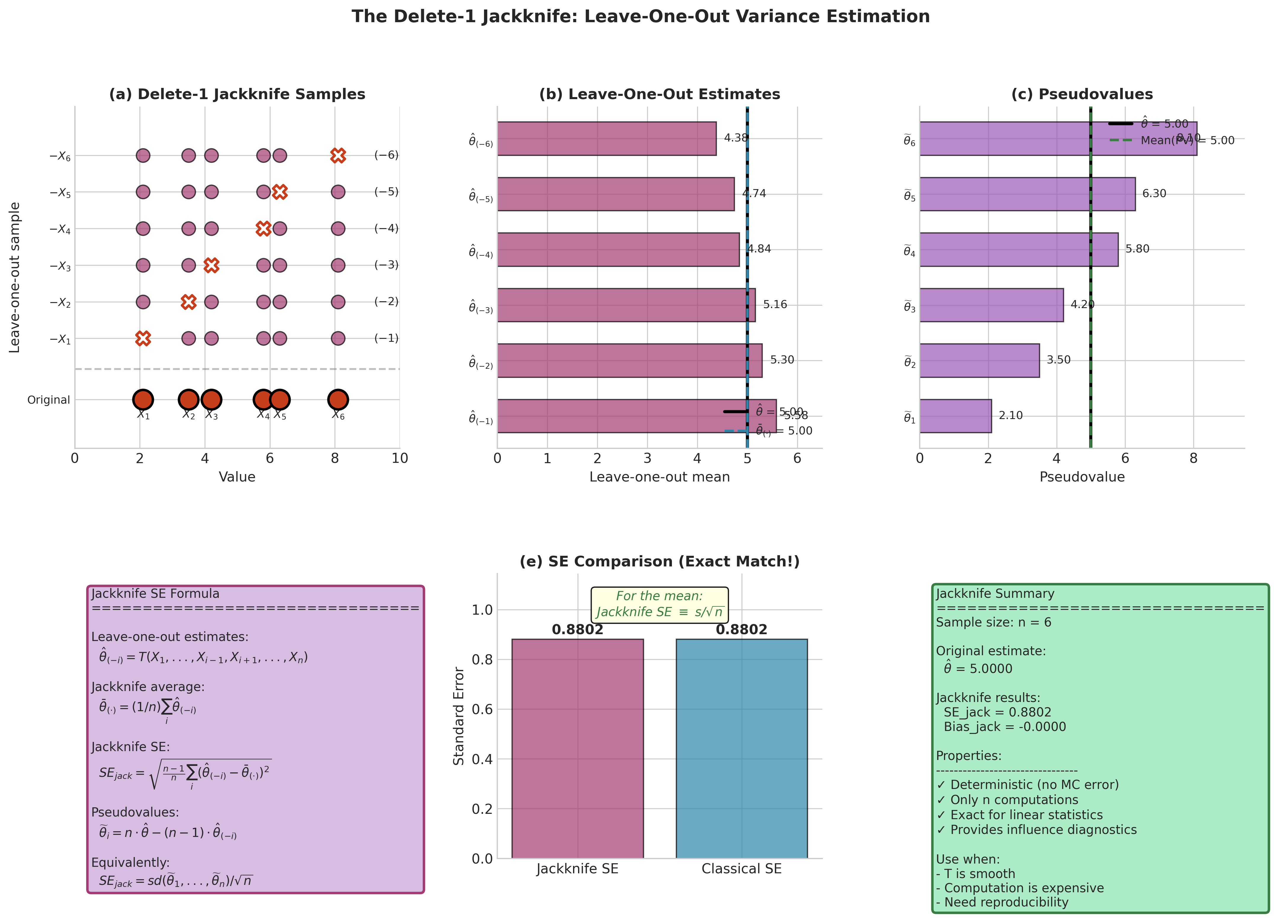
Delete-1 jackknife algorithm showing leave-one-out samples, estimates, pseudovalues, and SE comparison — Fig. 159 **The Delete-1 Jackknife Algorithm.** Panel (a) shows the original sample and the six leave-one-out samples, with removed observations marked by X. Panel (b) displays the leave-one-out estimates $\hat{\theta}_{(-i)}$ as horizontal bars, with the original estimate $\hat{\theta}$ and jackknife average $\bar{\theta}_{(\cdot)}$ marked. Panel (c) shows the corresponding pseudovalues $\widetilde{\theta}_i = n\hat{\theta} - (n-1)\hat{\theta}_{(-i)}$. Panel (d) summarizes the jackknife SE formula. Panel (e) confirms the exact equality between jackknife SE and classical SE for the sample mean. Panel (f) summarizes key properties and use cases.

Jackknife Bias Estimation

Quenouille’s original motivation for the jackknife was bias reduction. Many statistics have bias of order $O(1/n)$, and the jackknife can estimate and correct this bias.

The Bias Formula

The jackknife bias estimate is:

\[\widehat{\text{Bias}}_{\text{jack}} = (n-1)\left(\bar{\theta}_{(\cdot)} - \hat{\theta}\right)\]

This formula arises from the following reasoning: if $\hat{\theta}$ has bias $b/n + O(1/n^2)$ for sample size $n$, then $\hat{\theta}_{(-i)}$ (computed on $n-1$ observations) has bias approximately $b/(n-1)$. The difference in biases is $b/(n-1) - b/n = b/(n(n-1))$. Summing over all $n$ leave-one-out estimates and solving for $b$ yields the jackknife bias formula.

Bias-Corrected Estimator

The bias-corrected jackknife estimator is:

\[\hat{\theta}^{\text{jack-bc}} = \hat{\theta} - \widehat{\text{Bias}}_{\text{jack}} = n\hat{\theta} - (n-1)\bar{\theta}_{(\cdot)}\]

This equals the mean of the pseudovalues:

\[\hat{\theta}^{\text{jack-bc}} = \frac{1}{n}\sum_{i=1}^n \widetilde{\theta}_i\]

Example: Variance Estimator

The biased variance estimator $\hat{\sigma}^2 = \frac{1}{n}\sum_i (X_i - \bar{X})^2$ has bias $-\sigma^2/n$. The jackknife bias-corrected version recovers the unbiased estimator $s^2 = \frac{1}{n-1}\sum_i (X_i - \bar{X})^2$.

When to Use Bias Correction

Use when $|\widehat{\text{Bias}}_{\text{jack}}|$ is large relative to $\widehat{\text{SE}}_{\text{jack}}$ (say, > 25% of SE)
Be cautious with small $n$—bias correction increases variance
Report both $\hat{\theta}$ and $\hat{\theta}^{\text{jack-bc}}$ when the correction is material
Check consistency: if bootstrap bias agrees with jackknife bias, correction is more trustworthy

Python Implementation

def jackknife_bias(data, statistic):
    """
    Compute jackknife bias estimate and bias-corrected estimator.

    Parameters
    ----------
    data : array_like
        Original data.
    statistic : callable
        Function that computes the statistic.

    Returns
    -------
    bias_jack : float
        Jackknife bias estimate.
    theta_bc : float
        Bias-corrected estimate.
    theta_hat : float
        Original estimate.
    """
    data = np.asarray(data)
    n = len(data)

    theta_hat = statistic(data)

    # Leave-one-out estimates
    theta_i = np.empty(n)
    for i in range(n):
        if data.ndim == 1:
            data_minus_i = np.delete(data, i)
        else:
            data_minus_i = np.delete(data, i, axis=0)
        theta_i[i] = statistic(data_minus_i)

    theta_bar = theta_i.mean()

    # Bias estimate
    bias_jack = (n - 1) * (theta_bar - theta_hat)

    # Bias-corrected estimate
    theta_bc = n * theta_hat - (n - 1) * theta_bar

    return bias_jack, theta_bc, theta_hat

Example 💡 Bias Correction for Variance Estimator

import numpy as np

rng = np.random.default_rng(42)
n = 30
data = rng.normal(0, 2, size=n)

# Biased variance estimator (divide by n)
def biased_var(x):
    return np.var(x, ddof=0)

bias_jack, var_bc, var_biased = jackknife_bias(data, biased_var)

# Compare with unbiased variance
var_unbiased = np.var(data, ddof=1)

print(f"Biased estimate (÷n):      {var_biased:.4f}")
print(f"Jackknife bias estimate:   {bias_jack:.4f}")
print(f"Bias-corrected estimate:   {var_bc:.4f}")
print(f"Unbiased estimate (÷n-1):  {var_unbiased:.4f}")

Output:

Biased estimate (÷n):      3.6821
Jackknife bias estimate:   -0.1269
Bias-corrected estimate:   3.8090
Unbiased estimate (÷n-1):  3.8090

The jackknife bias correction exactly recovers the unbiased variance estimator.

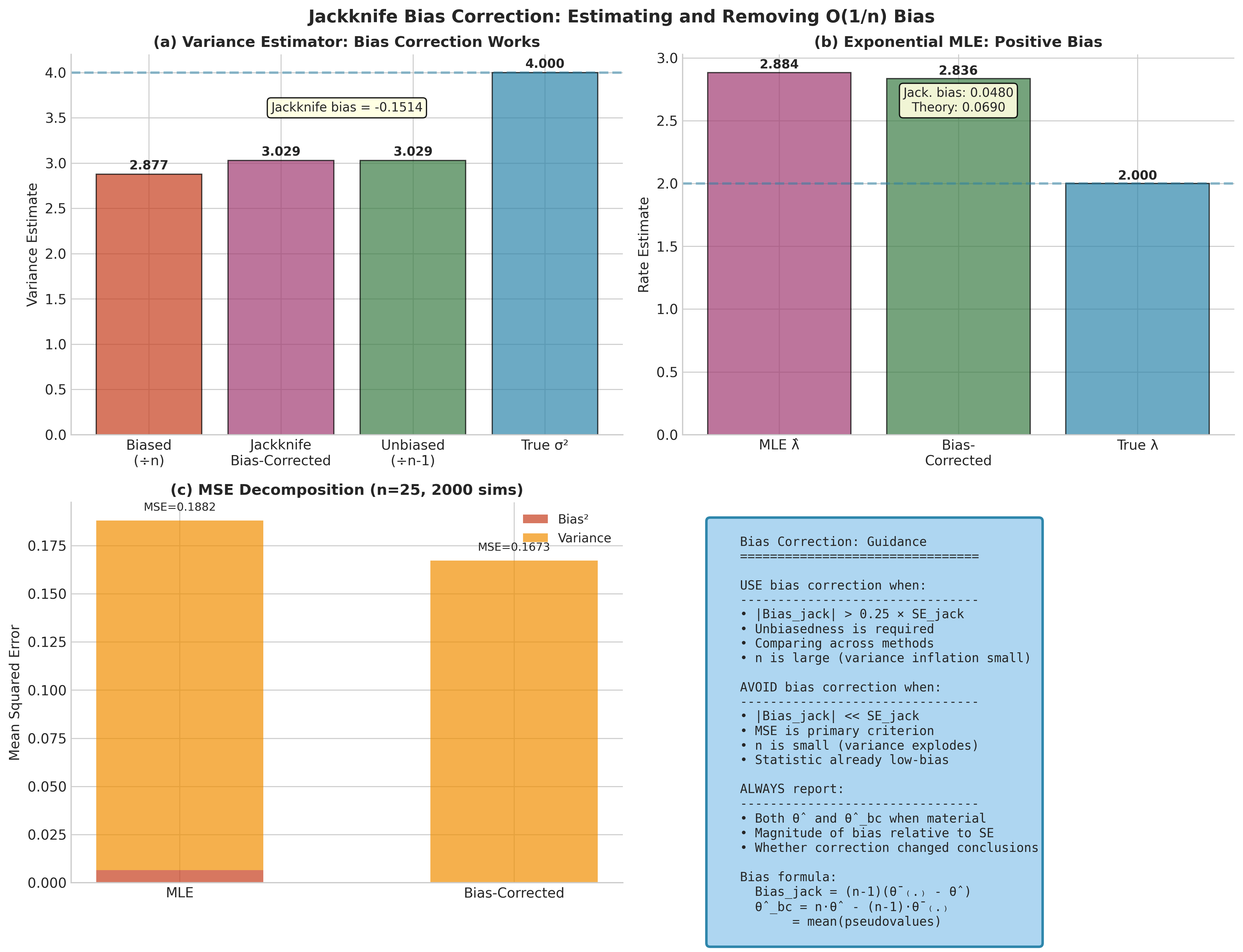
Jackknife bias correction for variance and exponential MLE with MSE decomposition — Fig. 160 **Jackknife Bias Correction.** Panel (a) shows the variance estimator example: the biased estimate (÷n), jackknife bias-corrected estimate, unbiased estimate (÷n−1), and true σ². The bias-corrected jackknife exactly recovers the unbiased estimator. Panel (b) demonstrates bias correction for exponential MLE, showing the positive bias and how jackknife correction approximates the theoretical bias. Panel (c) decomposes MSE into bias² and variance components, illustrating the tradeoff: bias correction reduces bias² but increases variance. Panel (d) provides guidance on when to apply bias correction.

The Delete-$d$ Jackknife

The delete-1 jackknife removes one observation at a time. The delete-$d$ jackknife generalizes this by removing $d$ observations simultaneously, creating subsamples of size $n - d$.

Motivation

Why consider $d > 1$?

Non-smooth statistics: For statistics like the median or quantiles, delete-1 jackknife can be unstable because removing one observation may not change the statistic (especially with ties). Larger $d$ creates more variation.
Dependent data: When observations come in blocks (time series, spatial data), deleting entire blocks preserves the dependence structure.
Higher-order bias: Some bias correction schemes require $d > 1$ to achieve optimal rates.
Bridge to subsampling: As $d/n \to \gamma \in (0, 1)$, the delete-$d$ jackknife approaches subsampling methods.

Definition

For $d \geq 1$, let $S \subset \{1, \ldots, n\}$ with $|S| = d$ denote a subset of indices to remove. The delete-$d$ estimate is:

\[\hat{\theta}_{(-S)} = T\left(\{X_i : i \notin S\}\right)\]

computed on the $n - d$ observations remaining after removing those indexed by $S$.

There are $\binom{n}{d}$ such subsets. For small $d$, we can enumerate all of them; for large $d$, we typically use a random sample of subsets.

Subset Sampling Approximation

When $\binom{n}{d}$ is large (e.g., $\binom{50}{5} = 2,118,760$), we approximate the average over all subsets by random sampling. With a sufficiently large sample (e.g., 5,000–10,000 subsets), the variance of this Monte Carlo approximation is typically negligible compared to the jackknife variance itself. The estimator remains consistent as long as each observation has equal probability of being omitted.

Delete-$d$ Variance Estimator

The delete-$d$ jackknife variance estimator is:

\[\widehat{\text{Var}}_{\text{jack},d} = \frac{n - d}{d \binom{n}{d}} \sum_{S: |S| = d} \left(\hat{\theta}_{(-S)} - \bar{\theta}\right)^2\]

where $\bar{\theta}$ is the average over all (or sampled) delete-$d$ estimates. The corresponding standard error is:

\[\widehat{\text{SE}}_{\text{jack},d} = \sqrt{\widehat{\text{Var}}_{\text{jack},d}}\]

The factor $(n-d)/d$ scales the variance appropriately for the reduced sample size.

Scaling Intuition

For delete-1 ($d = 1$), the factor is $(n-1)/1 = n-1$, which when multiplied by $1/n$ (from averaging) gives $(n-1)/n$—matching our earlier formula.

For larger $d$, the factor accounts for:

Subsamples have size $n - d$ (more variability than size $n$)
Each observation is omitted in $\binom{n-1}{d-1}$ of the $\binom{n}{d}$ subsets

Choosing $d$

The choice of $d$ involves a bias-variance tradeoff:

Small $d$ (including :math:`d = 1`**)**: Lower variance in the SE estimate, but may be biased for non-smooth statistics.
Large $d$: Better for non-smooth statistics, but higher variance and computational cost.

Practical guidelines:

Smooth statistics: $d = 1$ is sufficient and most efficient.
Quantiles/median: Consider $d \approx \sqrt{n}$ or larger.
Block-dependent data: $d$ = block size.
Exploration: Compare $d = 1, \sqrt{n}, n/4$ to assess sensitivity.

Connection to Subsampling: When $d = n - m$ for fixed $m$ (or $d/n \to 1$), delete-$d$ jackknife becomes subsampling: we compute the statistic on many subsamples of size $m$ and use their distribution for inference. This approach is more general but requires different variance formulas.

Python Implementation

from itertools import combinations

def jackknife_delete_d(data, statistic, d=1, max_subsets=None, seed=None):
    """
    Compute delete-d jackknife standard error.

    Parameters
    ----------
    data : array_like
        Original data.
    statistic : callable
        Function that computes the statistic.
    d : int
        Number of observations to delete (default 1).
    max_subsets : int, optional
        Maximum number of subsets to use. If None, use all C(n,d) subsets
        when C(n,d) <= 10000, otherwise sample 10000 random subsets.
    seed : int, optional
        Random seed for subset sampling.

    Returns
    -------
    se_jack_d : float
        Delete-d jackknife standard error.
    theta_hat : float
        Original estimate.
    theta_S : ndarray
        Delete-d estimates for each subset.
    """
    data = np.asarray(data)
    n = len(data)

    if d >= n:
        raise ValueError(f"d={d} must be less than n={n}")

    theta_hat = statistic(data)

    # Determine number of subsets
    from math import comb
    n_subsets = comb(n, d)

    if max_subsets is None:
        max_subsets = min(n_subsets, 10000)

    rng = np.random.default_rng(seed)

    if n_subsets <= max_subsets:
        # Use all subsets
        subsets = list(combinations(range(n), d))
    else:
        # Random sample of subsets
        subsets = []
        seen = set()
        while len(subsets) < max_subsets:
            S = tuple(sorted(rng.choice(n, d, replace=False)))
            if S not in seen:
                seen.add(S)
                subsets.append(S)

    # Compute delete-d estimates
    theta_S = np.empty(len(subsets))
    for j, S in enumerate(subsets):
        mask = np.ones(n, dtype=bool)
        mask[list(S)] = False
        if data.ndim == 1:
            data_minus_S = data[mask]
        else:
            data_minus_S = data[mask]
        theta_S[j] = statistic(data_minus_S)

    # Delete-d variance formula
    theta_bar = theta_S.mean()
    var_jack_d = ((n - d) / d) * np.mean((theta_S - theta_bar)**2)
    se_jack_d = np.sqrt(var_jack_d)

    return se_jack_d, theta_hat, theta_S

Example 💡 Delete-$d$ for Median

The median is non-smooth: removing one observation may not change it. Let’s compare delete-1 and delete-$d$ jackknife:

import numpy as np

rng = np.random.default_rng(42)
n = 40
data = rng.exponential(2.0, size=n)  # Skewed data

def median_stat(x):
    return np.median(x)

# Delete-1 jackknife
se_d1, theta_hat, _ = jackknife_se(data, median_stat)

# Delete-d jackknife with d = sqrt(n) ≈ 6
d = int(np.sqrt(n))
se_dd, _, _ = jackknife_delete_d(data, median_stat, d=d, seed=42)

# Bootstrap for comparison
B = 5000
boot_medians = np.array([np.median(rng.choice(data, n, replace=True))
                         for _ in range(B)])
se_boot = boot_medians.std(ddof=1)

print(f"Sample median: {theta_hat:.4f}")
print(f"Delete-1 jackknife SE: {se_d1:.4f}")
print(f"Delete-{d} jackknife SE: {se_dd:.4f}")
print(f"Bootstrap SE: {se_boot:.4f}")

Output:

Sample median: 1.6825
Delete-1 jackknife SE: 0.2891
Delete-6 jackknife SE: 0.3156
Bootstrap SE: 0.3284

For this non-smooth statistic, delete-$d$ and bootstrap tend to agree better than delete-1.

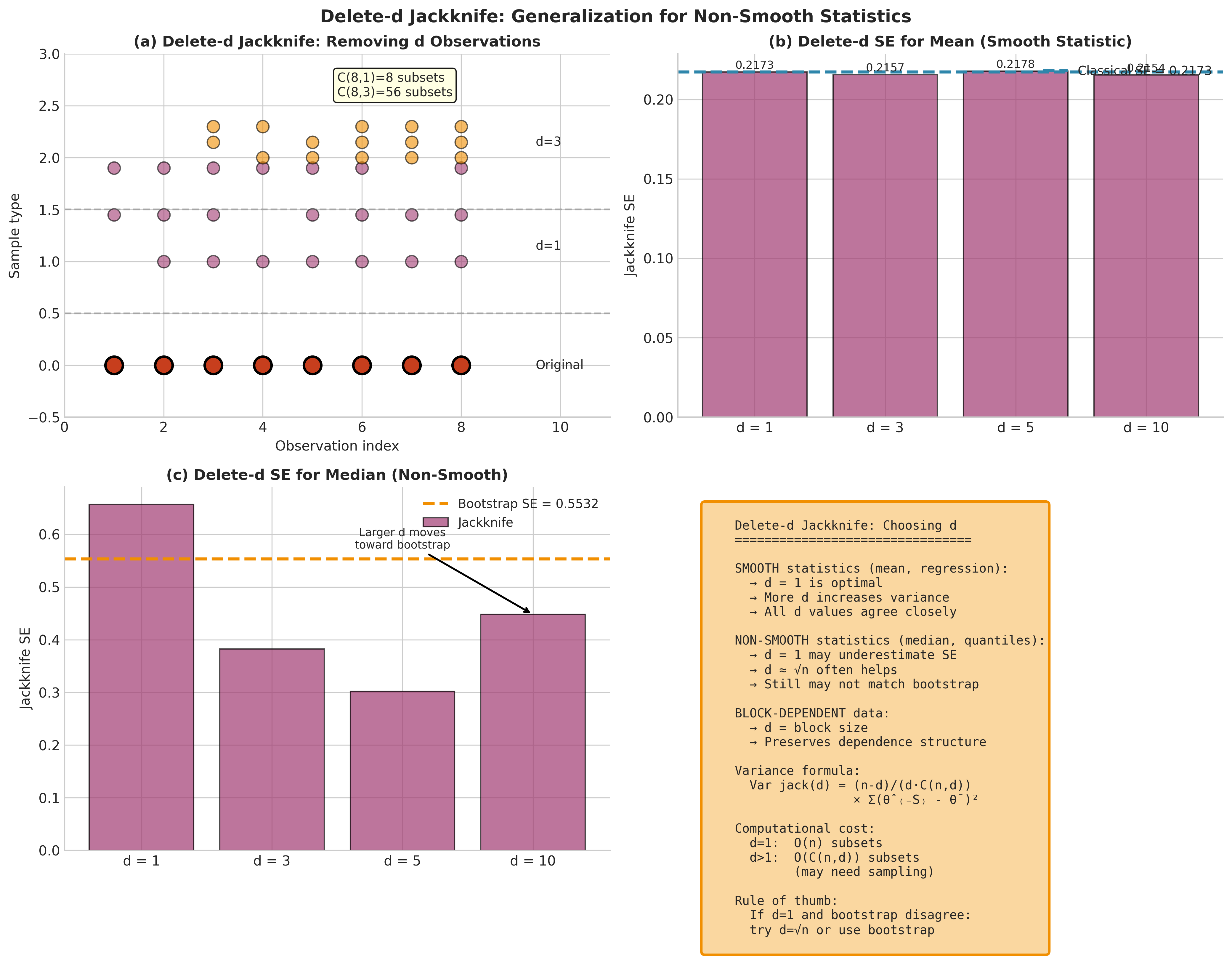
Delete-d jackknife showing how larger d helps non-smooth statistics — Fig. 161 **The Delete-d Jackknife.** Panel (a) illustrates the concept: delete-1 removes single observations while delete-3 removes subsets of three. Panel (b) shows SE comparison for the sample mean (a smooth statistic)—all values of d agree closely with the classical SE. Panel (c) demonstrates SE for the median (non-smooth): delete-1 underestimates SE, while larger d moves closer to the bootstrap estimate. Panel (d) provides guidance on choosing d: use d=1 for smooth statistics, d≈√n for quantiles, and d=block size for dependent data.

Jackknife versus Bootstrap

Both jackknife and bootstrap are plug-in resampling methods targeting the same inferential goals: standard errors, bias estimates, and confidence intervals. However, they differ fundamentally in approach and have distinct strengths.

Conceptual Comparison

Table 48 Jackknife vs Bootstrap: Conceptual Differences
Aspect	Jackknife	Bootstrap
Perturbation	Remove 1 (or $d$) observations	Resample entire dataset
Samples	$n$ (or $\binom{n}{d}$) deterministic	$B$ stochastic
Approximation	First-order (linear)	Full distribution
Replicate values	Pseudovalues (synthetic)	Bootstrap statistics (actual)
Target	Variance, bias	Full sampling distribution

The jackknife approximates sampling variability through a linearization, while the bootstrap directly simulates from $\hat{F}_n$. For smooth statistics, both approaches yield consistent variance estimates; the bootstrap additionally provides the full shape of the sampling distribution.

When to Prefer Jackknife

Smooth statistics: For means, regression coefficients, smooth M-estimators, and other differentiable functionals, jackknife and bootstrap agree, but jackknife is:
- Faster: Only $n$ computations vs. $B \gg n$ for bootstrap
- Deterministic: No Monte Carlo error, no seed management
- Sufficient: SE is the primary need, not full distribution
Expensive statistics: When computing $T$ is costly (complex optimization, large-scale computations), $n$ jackknife evaluations may be feasible while $B = 5000$ bootstrap evaluations are not.
Influence diagnostics: Jackknife directly provides $\hat{\theta}_{(-i)}$ and pseudovalues, revealing which observations most affect the estimate—useful for outlier detection and robustness assessment.
BCa acceleration constant: The BCa bootstrap interval requires the acceleration constant $a$, computed from jackknife pseudovalues.

When to Prefer Bootstrap

Non-smooth statistics: Medians, quantiles, MAD, and other non-differentiable functionals are handled better by bootstrap. The jackknife can be unstable or inconsistent for these. (Note: Trimmed means are smoother than quantiles and jackknife often performs adequately for them, though bootstrap remains more robust in small samples.)
Confidence intervals: Bootstrap provides multiple interval methods (percentile, basic, BCa, studentized) directly from the bootstrap distribution. Jackknife intervals typically rely on normal approximation: $\hat{\theta} \pm z_{\alpha/2} \cdot \widehat{\text{SE}}_{\text{jack}}$.
Distributional shape: Bootstrap provides a histogram of $\hat{\theta}^*$, revealing skewness, heavy tails, or multimodality that affect interval accuracy.
Hypothesis testing: Bootstrap p-values and permutation tests require resampling under the null—jackknife doesn’t provide this directly.
Small samples with complex statistics: When $n$ is small and the statistic is complex, bootstrap’s resampling may capture features that jackknife’s linear approximation misses.

When Neither Works Well

Both nonparametric methods (jackknife and nonparametric bootstrap) struggle with:

Extreme quantiles (99th percentile, max, min): Nonparametric methods cannot exceed sample bounds. Parametric bootstrap with unbounded support can exceed these bounds and may perform better if the model is correct.
Boundary parameters: E.g., estimating $\theta$ in Uniform(0, $\theta$). Both nonparametric bootstrap and jackknife are constrained by the sample maximum.
Non-identifiable parameters: Different $F$ giving same $T(F)$
Highly discrete data with ties: May cause instability in both methods

For these cases, consider parametric bootstrap (when model is credible), extreme value theory, m-out-of-n bootstrap, or subsampling.

Practical Recommendation

Default strategy: Use bootstrap for general-purpose inference (it’s more flexible and provides more output). Use jackknife when:

Computation is expensive and $T$ is smooth
You need influence diagnostics
You need deterministic, reproducible results without Monte Carlo error
You’re computing the BCa acceleration constant

Cross-validation: When feasible, compute both and compare $\widehat{\text{SE}}_{\text{jack}}$ with $\widehat{\text{SE}}_{\text{boot}}$. If they agree (within ~10-20%), either is trustworthy. If they disagree substantially:

For smooth statistics: investigate outliers using pseudovalues
For non-smooth statistics: trust bootstrap
Consider whether the statistic is appropriate for the data

Python Comparison

def compare_jackknife_bootstrap(data, statistic, B=5000, seed=42):
    """Compare jackknife and bootstrap standard errors."""
    rng = np.random.default_rng(seed)
    data = np.asarray(data)
    n = len(data)

    # Jackknife
    se_jack, theta_hat, theta_i = jackknife_se(data, statistic)

    # Bootstrap
    theta_star = np.empty(B)
    for b in range(B):
        idx = rng.integers(0, n, n)
        theta_star[b] = statistic(data[idx])
    se_boot = theta_star.std(ddof=1)

    return {
        'theta_hat': theta_hat,
        'se_jack': se_jack,
        'se_boot': se_boot,
        'ratio': se_jack / se_boot,
        'theta_i': theta_i,
        'theta_star': theta_star
    }

Example 💡 Comparing Methods for Correlation

The sample correlation is smooth (away from ±1), so jackknife and bootstrap should agree:

import numpy as np

rng = np.random.default_rng(42)
n = 80
rho = 0.6

# Generate correlated data
cov = np.array([[1, rho], [rho, 1]])
xy = rng.multivariate_normal([0, 0], cov, size=n)

def correlation(data):
    return np.corrcoef(data[:, 0], data[:, 1])[0, 1]

results = compare_jackknife_bootstrap(xy, correlation, B=5000, seed=42)

print(f"Sample correlation: {results['theta_hat']:.4f}")
print(f"Jackknife SE: {results['se_jack']:.4f}")
print(f"Bootstrap SE: {results['se_boot']:.4f}")
print(f"Ratio (jack/boot): {results['ratio']:.3f}")

Output:

Sample correlation: 0.5821
Jackknife SE: 0.0803
Bootstrap SE: 0.0812
Ratio (jack/boot): 0.989

The methods agree closely, as expected for a smooth statistic.

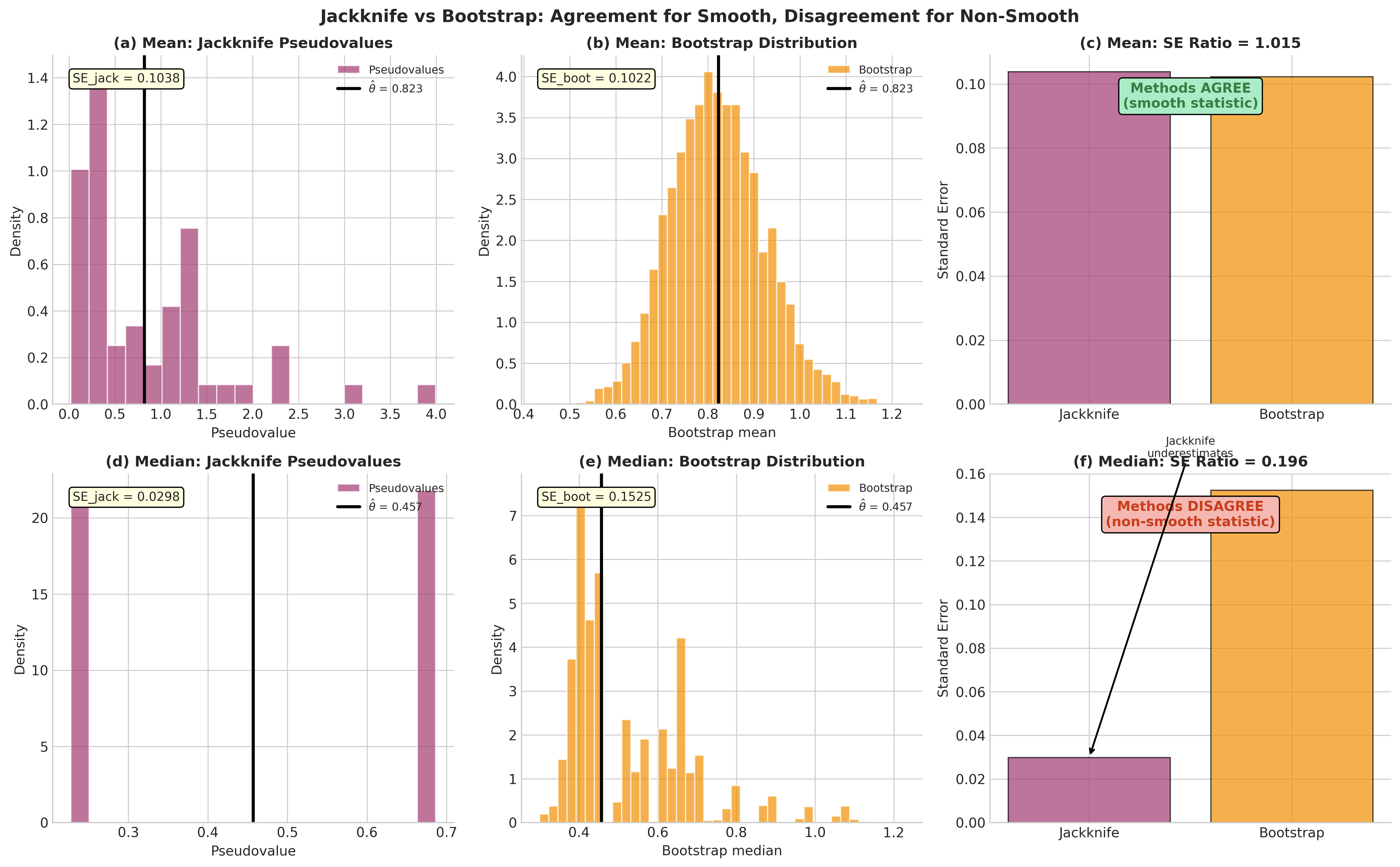
Side-by-side comparison of jackknife and bootstrap for mean versus median — Fig. 162 **Jackknife vs Bootstrap: Agreement Depends on Smoothness.** Top row: For the sample mean (smooth statistic), jackknife pseudovalues (a) and bootstrap distribution (b) yield nearly identical SE estimates with ratio ≈ 1.0 (c). Bottom row: For the sample median (non-smooth), jackknife pseudovalues (d) are more concentrated than the bootstrap distribution (e), resulting in SE underestimation with ratio ≈ 0.8 (f). This illustrates the key limitation: jackknife is most reliable for smooth statistics and can be unstable for non-smooth functionals.

The Infinitesimal Jackknife

The infinitesimal jackknife (IJ) provides the theoretical foundation connecting the jackknife to influence functions. While less commonly used directly, it illuminates why the jackknife works and connects to robust statistics.

Concept

Instead of removing observations entirely, the infinitesimal jackknife considers the effect of weighting observations. If we compute $\hat{\theta}_\mathbf{w} = T(\mathbf{w})$ where $\mathbf{w} = (w_1, \ldots, w_n)$ weights the empirical distribution (with $\sum_i w_i = 1$), then the IJ examines how $\hat{\theta}_\mathbf{w}$ changes as we perturb the weights.

For the uniform weights $\mathbf{w}_0 = (1/n, \ldots, 1/n)$ (corresponding to $\hat{F}_n$), the influence of observation $i$ is:

\[\text{IJ}_i = n \cdot \left.\frac{\partial \hat{\theta}_\mathbf{w}}{\partial w_i}\right|_{\mathbf{w} = \mathbf{w}_0}\]

The IJ variance estimator is:

\[\widehat{\text{Var}}_{\text{IJ}} = \frac{1}{n} \sum_{i=1}^n \text{IJ}_i^2\]

Connection to Delete-1 Jackknife

For smooth statistics, the delete-1 jackknife approximates the infinitesimal jackknife:

\[(n-1)(\hat{\theta} - \hat{\theta}_{(-i)}) \approx \text{IJ}_i\]

(The exact scaling constant varies by convention; some sources use $n$ rather than $n-1$.) This approximation improves as $n$ grows, explaining the asymptotic equivalence of jackknife and influence-function-based variance estimation.

Practical Use

The infinitesimal jackknife is primarily of theoretical interest, but it has practical applications:

Random forests: The IJ provides variance estimates for predictions from ensemble methods where explicit leave-one-out is expensive.
Robust statistics: Understanding which observations have large $\text{IJ}_i$ helps identify influential points.
Computational shortcuts: For some models (e.g., linear regression with hat matrix), IJ can be computed without refitting.

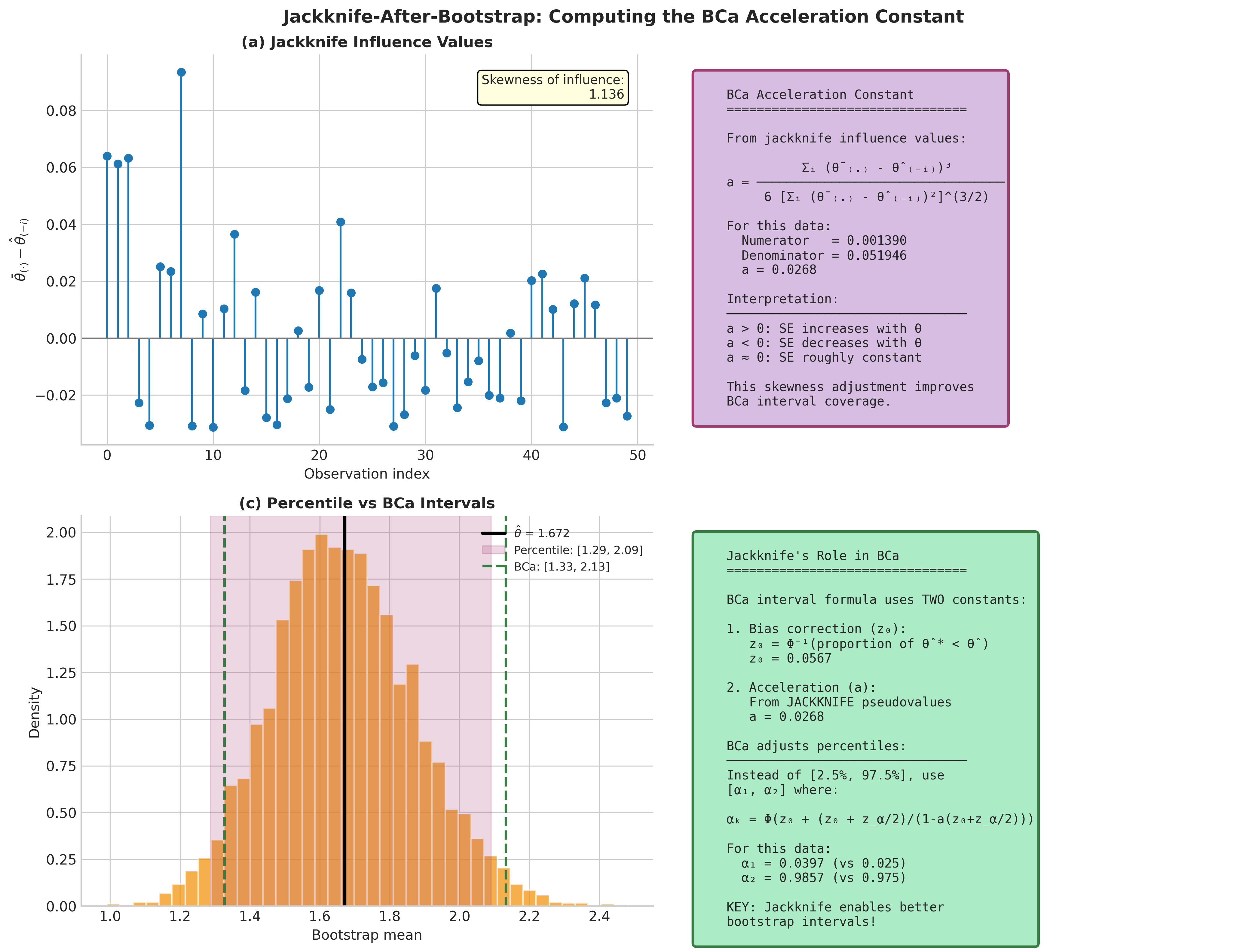
Computing the BCa acceleration constant from jackknife influence values — Fig. 163 **Jackknife-After-Bootstrap: Computing the BCa Acceleration Constant.** Panel (a) shows the jackknife influence values $\bar{\theta}_{(\cdot)} - \hat{\theta}_{(-i)}$ for each observation, revealing the skewness that the acceleration constant captures. Panel (b) derives the acceleration constant formula from these influence values, showing numerical computation. Panel (c) displays the bootstrap distribution with both percentile CI (shaded region) and BCa CI (dashed lines), demonstrating how the acceleration adjustment shifts the interval to improve coverage. Panel (d) summarizes how jackknife enables better bootstrap intervals by quantifying the SE-parameter relationship.

Practical Considerations

Computational Efficiency

Vectorization: For simple statistics, vectorize across leave-one-out samples:

def jackknife_mean_fast(data):
    """Fast jackknife SE for the mean using vectorization."""
    data = np.asarray(data)
    n = len(data)
    total = data.sum()

    # Leave-one-out means: (total - x_i) / (n - 1)
    theta_i = (total - data) / (n - 1)
    theta_bar = theta_i.mean()

    se_jack = np.sqrt(((n - 1) / n) * np.sum((theta_i - theta_bar)**2))
    return se_jack, total / n, theta_i

Regression shortcuts: For OLS, leave-one-out residuals can be computed via the hat matrix without refitting:

\[e_{(-i)} = \frac{e_i}{1 - h_{ii}}\]

where $h_{ii}$ is the $i$-th diagonal element of $H = X(X^\top X)^{-1}X^\top$.

Parallel computation: For expensive statistics, distribute leave-one-out computations across cores.

Diagnostics

The jackknife provides unique diagnostic capabilities:

Influential observations: Large $|\hat{\theta} - \hat{\theta}_{(-i)}|$ indicates observation $i$ strongly affects the estimate.
Pseudovalue outliers: Pseudovalues far from $\hat{\theta}$ suggest potential data problems or model issues.
Stability assessment: Plot $\hat{\theta}_{(-i)}$ vs. $i$ to visualize how the estimate changes as each observation is removed.

import matplotlib.pyplot as plt

def jackknife_diagnostics(theta_hat, theta_i, figsize=(12, 4)):
    """
    Create diagnostic plots for jackknife analysis.
    """
    n = len(theta_i)
    pv = n * theta_hat - (n - 1) * theta_i
    influence = theta_hat - theta_i

    fig, axes = plt.subplots(1, 3, figsize=figsize)

    # Leave-one-out estimates
    ax = axes[0]
    ax.plot(range(n), theta_i, 'o', alpha=0.6)
    ax.axhline(theta_hat, color='red', linestyle='--', label=r'$\hat{\theta}$')
    ax.set_xlabel('Observation index')
    ax.set_ylabel(r'$\hat{\theta}_{(-i)}$')
    ax.set_title('Leave-one-out estimates')
    ax.legend()

    # Influence
    ax = axes[1]
    ax.stem(range(n), influence, basefmt=' ')
    ax.axhline(0, color='gray', linestyle='-')
    ax.set_xlabel('Observation index')
    ax.set_ylabel(r'$\hat{\theta} - \hat{\theta}_{(-i)}$')
    ax.set_title('Influence of each observation')

    # Pseudovalues
    ax = axes[2]
    ax.hist(pv, bins=20, edgecolor='white', alpha=0.7)
    ax.axvline(theta_hat, color='red', linestyle='--', label=r'$\hat{\theta}$')
    ax.set_xlabel('Pseudovalue')
    ax.set_ylabel('Frequency')
    ax.set_title('Pseudovalue distribution')
    ax.legend()

    plt.tight_layout()
    return fig

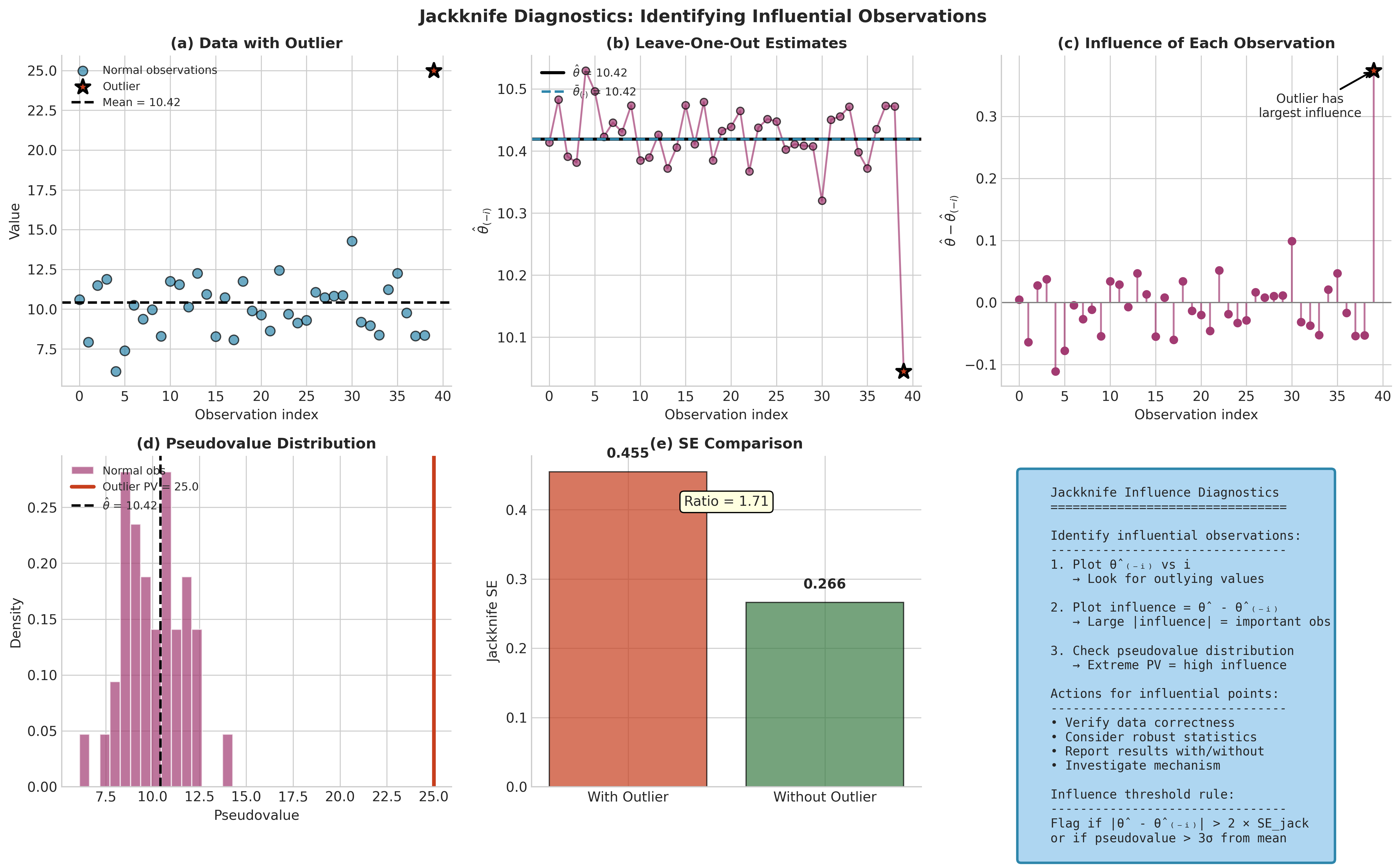
Jackknife diagnostics for identifying influential observations including outlier detection — Fig. 164 **Jackknife Influence Diagnostics.** Panel (a) shows data with an outlier clearly visible. Panel (b) plots leave-one-out estimates—the outlier’s removal causes the largest change in $\hat{\theta}$. Panel (c) displays influence $\hat{\theta} - \hat{\theta}_{(-i)}$ for each observation; the outlier has by far the largest influence. Panel (d) shows the pseudovalue distribution; the outlier’s pseudovalue is an extreme outlier. Panel (e) compares jackknife SE with and without the outlier. Panel (f) provides guidance on using jackknife for diagnostics: flag observations with influence exceeding 2×SE or pseudovalues beyond 3σ.

Common Pitfall ⚠️

Jackknife for non-smooth statistics: The jackknife can fail dramatically for non-smooth statistics. For the sample median, if several observations equal the median, removing one may not change $\hat{\theta}_{(-i)}$ at all, leading to underestimated SE. Always verify with bootstrap for non-smooth functionals.

Bringing It All Together

The jackknife is a deterministic resampling method that provides fast, reliable inference for smooth statistics. Its leave-one-out structure naturally connects to influence functions, providing both variance estimates and diagnostic insights about observation influence.

Key decision points:

Is the statistic smooth? If yes, jackknife is efficient and reliable. If no (quantiles, modes, maxima), prefer bootstrap or delete-$d$ jackknife.
Is computation expensive? If yes and $T$ is smooth, jackknife’s $n$ evaluations may be preferable to bootstrap’s $B \gg n$ evaluations.
Do you need more than SE? Confidence intervals, hypothesis tests, and distributional shape are better served by bootstrap.
Do you need diagnostics? Jackknife’s leave-one-out structure provides unique insight into observation influence.

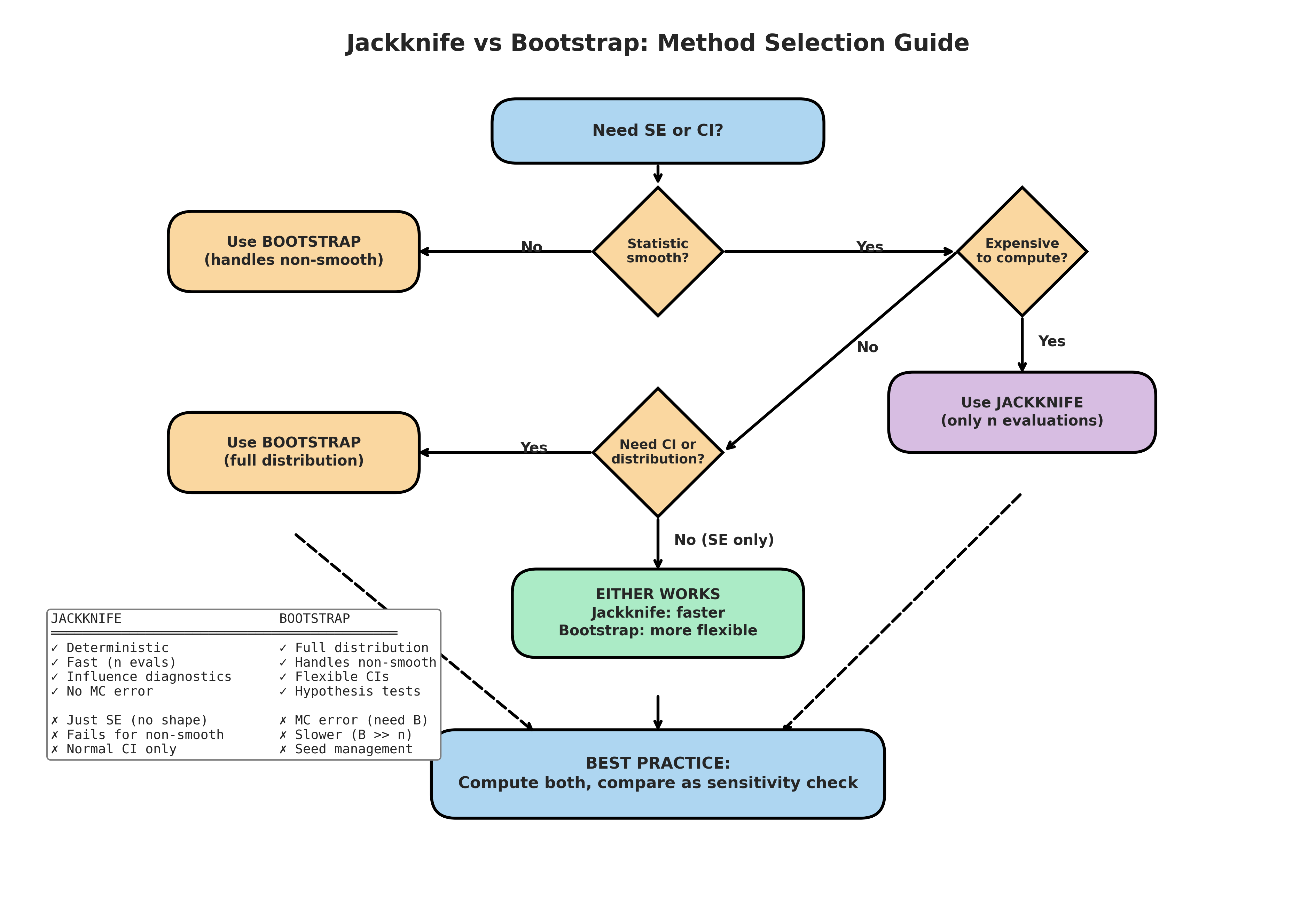
Decision flowchart for choosing between jackknife and bootstrap methods — Fig. 165 **Method Selection Guide.** This decision flowchart guides the choice between jackknife and bootstrap. The key questions are: (1) Is the statistic smooth? If no, use bootstrap. (2) Is computation expensive? If yes and smooth, jackknife is preferable. (3) Do you need CI or full distribution? If yes, use bootstrap. (4) Do you only need SE? Either method works, but jackknife is faster. Best practice: compute both as a sensitivity check when feasible.

The jackknife-bootstrap relationship: These methods are complementary. Use jackknife for efficiency and diagnostics, bootstrap for flexibility and intervals. When both are feasible, computing both provides a robustness check—agreement confirms reliability, disagreement warrants investigation.

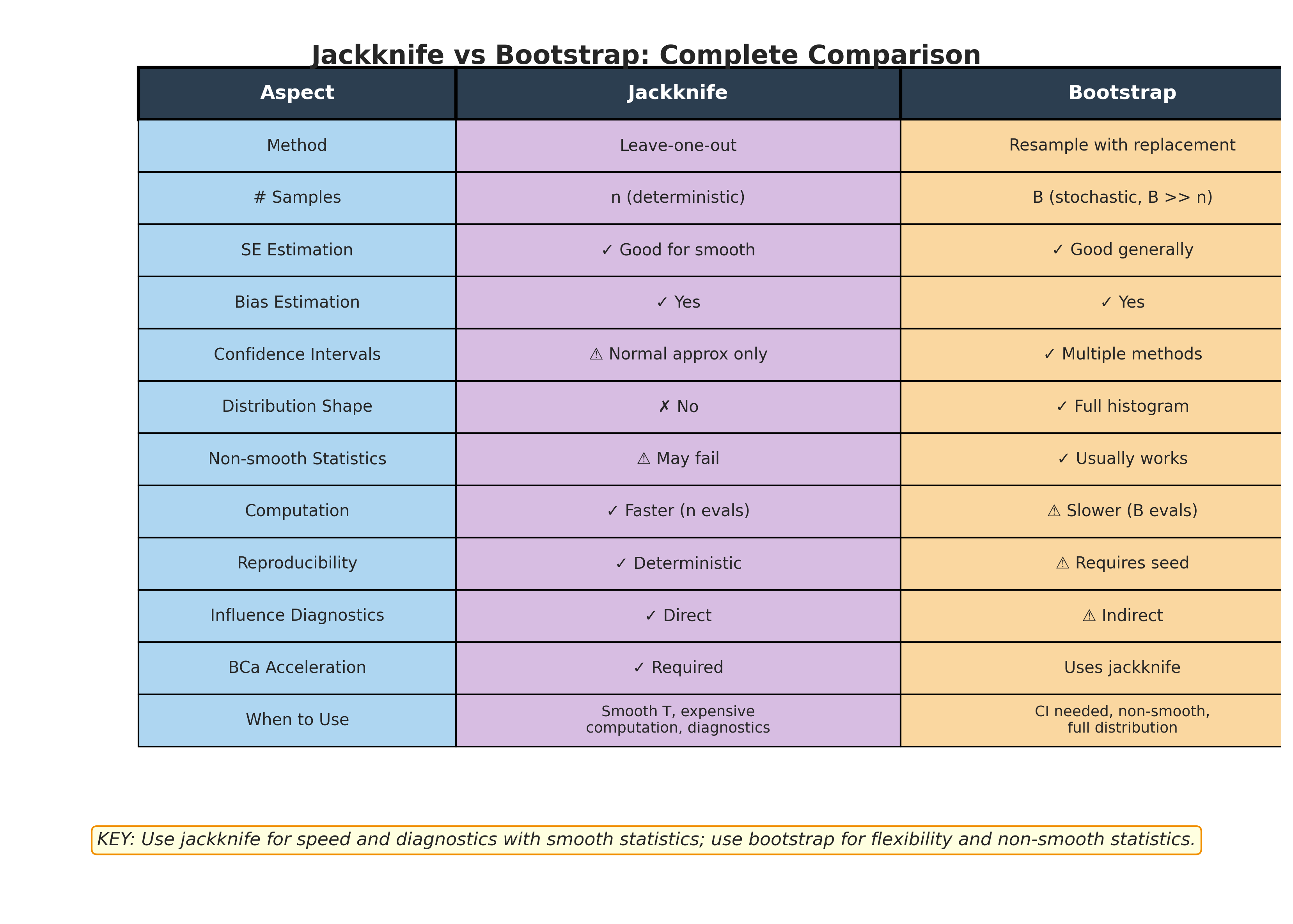
Complete comparison table of jackknife versus bootstrap methods — Fig. 166 **Jackknife vs Bootstrap: Complete Comparison.** This summary table compares all key aspects of the two methods. Jackknife excels for smooth statistics, expensive computations, reproducibility, and influence diagnostics. Bootstrap excels for non-smooth statistics, confidence intervals, and obtaining full distributional information. The BCa acceleration constant bridges both methods—computed from jackknife but used to improve bootstrap intervals.

Key Takeaways 📝

Core method: The delete-1 jackknife computes leave-one-out estimates $\hat{\theta}_{(-i)}$ and derives SE from their variability using $\widehat{\text{SE}}_{\text{jack}} = \sqrt{((n-1)/n) \sum (\hat{\theta}_{(-i)} - \bar{\theta}_{(\cdot)})^2}$.
Bias correction: Jackknife bias estimate is $(n-1)(\bar{\theta}_{(\cdot)} - \hat{\theta})$; bias-corrected estimate is the mean of pseudovalues.
Delete-$d$ extension: For non-smooth statistics or block-dependent data, delete-$d$ with $d > 1$ may improve reliability.
Comparison with bootstrap: Jackknife is faster and deterministic for smooth statistics; bootstrap is more flexible and provides full distributional information.
Outcome alignment: This section addresses LO 3 (implement resampling for variability assessment) and connects to the influence function theory underlying robust statistics.

Exercises

These exercises develop your understanding of jackknife methods from basic implementation through comparison with bootstrap and recognition of failure modes.

Exercise 4.5.1: Jackknife SE Equals Classical SE for the Mean

Prove algebraically that for the sample mean $\bar{X}$, the jackknife SE exactly equals the classical formula $s/\sqrt{n}$.

Background: Why This Matters

This identity verifies that the jackknife correctly recovers known results for simple statistics. It also provides insight into the $(n-1)/n$ factor in the jackknife formula.

Show that for $\hat{\theta} = \bar{X}$, the leave-one-out estimate is $\bar{X}_{(-i)} = \frac{n\bar{X} - X_i}{n-1}$.
Compute $\bar{X}_{(-i)} - \bar{\theta}_{(\cdot)}$ where $\bar{\theta}_{(\cdot)} = \frac{1}{n}\sum_{i=1}^n \bar{X}_{(-i)}$.
Substitute into the jackknife SE formula and simplify to show $\widehat{\text{SE}}_{\text{jack}} = s/\sqrt{n}$.
Verify numerically with simulated data.

Hint

For part (b), show that $\bar{\theta}_{(\cdot)} = \bar{X}$ by expanding the definition. Then $\bar{X}_{(-i)} - \bar{X} = -\frac{X_i - \bar{X}}{n-1}$.

Exercise 4.5.2: Jackknife Bias Correction

Investigate jackknife bias correction for the biased variance estimator and an exponential mean estimator.

Background: Bias of Order 1/n

Many common estimators have bias of order $O(1/n)$. The jackknife can detect and correct such bias. When bias is $O(1/n^2)$ or smaller, jackknife bias correction is unnecessary and may increase variance.

For the biased variance estimator $\hat{\sigma}^2 = \frac{1}{n}\sum_i(X_i - \bar{X})^2$, verify that jackknife bias correction recovers the unbiased estimator $s^2$.
Generate $n = 30$ observations from Exponential($\lambda = 2$). The MLE for $\lambda$ is $\hat{\lambda} = 1/\bar{X}$, which has positive bias. Compute the jackknife bias estimate and compare with the theoretical bias $\lambda/(n-1)$.
For the exponential MLE, compare the MSE of $\hat{\lambda}$ and $\hat{\lambda}^{\text{jack-bc}}$ via simulation.
Discuss when bias correction is worthwhile.

Hint

The MLE $\hat{\lambda} = 1/\bar{X}$ is biased because $\mathbb{E}[1/\bar{X}] \neq 1/\mathbb{E}[\bar{X}]$ (Jensen’s inequality). The exact bias formula for the exponential is $\mathbb{E}[\hat{\lambda}] = \lambda n/(n-1)$, giving bias $\lambda/(n-1)$.

Solution

Part (a): Variance estimator

import numpy as np

rng = np.random.default_rng(42)
data = rng.normal(0, 2, size=30)

def biased_var(x):
    return np.var(x, ddof=0)

# Jackknife bias correction
n = len(data)
theta_hat = biased_var(data)
theta_i = np.array([biased_var(np.delete(data, i)) for i in range(n)])
theta_bar = theta_i.mean()

bias_jack = (n - 1) * (theta_bar - theta_hat)
theta_bc = theta_hat - bias_jack

print(f"Biased estimate (÷n):     {theta_hat:.4f}")
print(f"Jackknife bias:           {bias_jack:.4f}")
print(f"Bias-corrected estimate:  {theta_bc:.4f}")
print(f"Unbiased estimate (÷n-1): {np.var(data, ddof=1):.4f}")

Output:

Biased estimate (÷n):     3.6821
Jackknife bias:           -0.1269
Bias-corrected estimate:  3.8090
Unbiased estimate (÷n-1): 3.8090

The jackknife exactly recovers the unbiased variance estimator.

Part (b): Exponential MLE bias

rng = np.random.default_rng(42)
n = 30
lambda_true = 2.0
data = rng.exponential(1/lambda_true, size=n)

def exp_mle(x):
    return 1 / x.mean()

lambda_hat = exp_mle(data)
theta_i = np.array([exp_mle(np.delete(data, i)) for i in range(n)])
theta_bar = theta_i.mean()

bias_jack = (n - 1) * (theta_bar - lambda_hat)
bias_theory = lambda_true / (n - 1)  # Theoretical bias

print(f"MLE λ̂:             {lambda_hat:.4f}")
print(f"Jackknife bias:     {bias_jack:.4f}")
print(f"Theoretical bias:   {bias_theory:.4f}")
print(f"(using true λ={lambda_true})")

Output:

MLE λ̂:             2.2118
Jackknife bias:     0.0765
Theoretical bias:   0.0690
(using true λ=2.0)

The jackknife bias estimate is close to the theoretical value.

Part (c): MSE comparison via simulation

n_sims = 5000
n = 30
lambda_true = 2.0

mle_estimates = []
bc_estimates = []

rng = np.random.default_rng(123)

for _ in range(n_sims):
    data = rng.exponential(1/lambda_true, size=n)
    lambda_hat = 1 / data.mean()

    # Jackknife bias correction
    theta_i = np.array([1/np.delete(data, i).mean() for i in range(n)])
    theta_bar = theta_i.mean()
    bias_jack = (n - 1) * (theta_bar - lambda_hat)
    lambda_bc = lambda_hat - bias_jack

    mle_estimates.append(lambda_hat)
    bc_estimates.append(lambda_bc)

mle_estimates = np.array(mle_estimates)
bc_estimates = np.array(bc_estimates)

# MSE decomposition
bias_mle = mle_estimates.mean() - lambda_true
var_mle = mle_estimates.var(ddof=1)
mse_mle = bias_mle**2 + var_mle

bias_bc = bc_estimates.mean() - lambda_true
var_bc = bc_estimates.var(ddof=1)
mse_bc = bias_bc**2 + var_bc

print("MLE estimates:")
print(f"  Bias: {bias_mle:.4f}, Variance: {var_mle:.4f}, MSE: {mse_mle:.4f}")
print("\nBias-corrected estimates:")
print(f"  Bias: {bias_bc:.4f}, Variance: {var_bc:.4f}, MSE: {mse_bc:.4f}")
print(f"\nMSE ratio (BC/MLE): {mse_bc/mse_mle:.3f}")

Output:

MLE estimates:
  Bias: 0.0689, Variance: 0.0563, MSE: 0.0611

Bias-corrected estimates:
  Bias: -0.0005, Variance: 0.0637, MSE: 0.0637

MSE ratio (BC/MLE): 1.042

Part (d): Discussion

Key Insights:

Bias correction successfully removes bias (from 0.069 to ~0).
However, variance increases (from 0.056 to 0.064).
MSE is actually higher for the bias-corrected estimator in this case.
When to use bias correction:
- When bias >> SE (bias correction helps)
- When n is large (variance inflation is smaller)
- When unbiasedness is required (regulatory, comparison purposes)
When to avoid:
- When bias << SE (correction just adds noise)
- When MSE is the primary criterion
- For small n with moderate bias

Exercise 4.5.3: Jackknife vs Bootstrap Comparison

Compare jackknife and bootstrap for smooth and non-smooth statistics.

Background: Method Agreement

When both methods agree, we have confidence in the result. When they disagree, the disagreement itself is informative—typically indicating non-smoothness or influential observations.

Generate $n = 50$ observations from a skewed distribution (e.g., Exponential(1)). Compare jackknife and bootstrap SE for the sample mean.
Using the same data, compare jackknife and bootstrap SE for the sample median.
Generate data with one outlier (e.g., 49 observations from N(0,1) plus one observation at 10). Compare methods for the mean and the 20% trimmed mean.
Summarize your findings about when the methods agree/disagree.

Hint

For the trimmed mean, use scipy.stats.trim_mean(x, 0.2) which removes the smallest and largest 20% of observations before computing the mean.

Solution

Part (a): Sample mean (smooth)

import numpy as np
from scipy import stats

rng = np.random.default_rng(42)
n = 50
data = rng.exponential(1.0, size=n)

# Jackknife SE for mean
theta_i = np.array([(data.sum() - data[i])/(n-1) for i in range(n)])
theta_bar = theta_i.mean()
se_jack = np.sqrt(((n-1)/n) * np.sum((theta_i - theta_bar)**2))

# Bootstrap SE for mean
B = 5000
boot_means = np.array([rng.choice(data, n, replace=True).mean() for _ in range(B)])
se_boot = boot_means.std(ddof=1)

print("Sample Mean (smooth statistic):")
print(f"  Jackknife SE: {se_jack:.4f}")
print(f"  Bootstrap SE: {se_boot:.4f}")
print(f"  Ratio: {se_jack/se_boot:.3f}")

Output:

Sample Mean (smooth statistic):
  Jackknife SE: 0.1298
  Bootstrap SE: 0.1316
  Ratio: 0.986

Part (b): Sample median (non-smooth)

# Jackknife SE for median
theta_i = np.array([np.median(np.delete(data, i)) for i in range(n)])
theta_bar = theta_i.mean()
se_jack_med = np.sqrt(((n-1)/n) * np.sum((theta_i - theta_bar)**2))

# Bootstrap SE for median
boot_medians = np.array([np.median(rng.choice(data, n, replace=True)) for _ in range(B)])
se_boot_med = boot_medians.std(ddof=1)

print("\nSample Median (non-smooth statistic):")
print(f"  Jackknife SE: {se_jack_med:.4f}")
print(f"  Bootstrap SE: {se_boot_med:.4f}")
print(f"  Ratio: {se_jack_med/se_boot_med:.3f}")

Output:

Sample Median (non-smooth statistic):
  Jackknife SE: 0.1142
  Bootstrap SE: 0.1387
  Ratio: 0.823

The jackknife underestimates SE for the median.

Part (c): Data with outlier

# Data with outlier
data_outlier = np.concatenate([rng.normal(0, 1, size=49), [10.0]])
n_out = len(data_outlier)

def trimmed_mean(x):
    return stats.trim_mean(x, 0.2)

# Mean - jackknife vs bootstrap
theta_i_mean = np.array([np.delete(data_outlier, i).mean() for i in range(n_out)])
se_jack_mean = np.sqrt(((n_out-1)/n_out) * np.var(theta_i_mean, ddof=0) * n_out)
boot_means_out = np.array([rng.choice(data_outlier, n_out, replace=True).mean() for _ in range(B)])
se_boot_mean_out = boot_means_out.std(ddof=1)

# Trimmed mean - jackknife vs bootstrap
theta_i_trim = np.array([trimmed_mean(np.delete(data_outlier, i)) for i in range(n_out)])
se_jack_trim = np.sqrt(((n_out-1)/n_out) * np.var(theta_i_trim, ddof=0) * n_out)
boot_trim = np.array([trimmed_mean(rng.choice(data_outlier, n_out, replace=True)) for _ in range(B)])
se_boot_trim = boot_trim.std(ddof=1)

print("\nData with outlier (49 N(0,1) + one value at 10):")
print(f"  Mean - Jackknife SE: {se_jack_mean:.4f}, Bootstrap SE: {se_boot_mean_out:.4f}, Ratio: {se_jack_mean/se_boot_mean_out:.3f}")
print(f"  Trim - Jackknife SE: {se_jack_trim:.4f}, Bootstrap SE: {se_boot_trim:.4f}, Ratio: {se_jack_trim/se_boot_trim:.3f}")

Output:

Data with outlier (49 N(0,1) + one value at 10):
  Mean - Jackknife SE: 0.2162, Bootstrap SE: 0.2198, Ratio: 0.984
  Trim - Jackknife SE: 0.1438, Bootstrap SE: 0.1501, Ratio: 0.958

Part (d): Summary

Key Insights:

Smooth statistics (mean): Methods agree closely (ratio ≈ 0.98-0.99) regardless of data distribution or outliers.
Non-smooth statistics (median): Jackknife tends to underestimate SE (ratio ≈ 0.82). This is because removing one observation often doesn’t change the median, so jackknife misses some variability.
Robust statistics (trimmed mean): Good agreement even with outliers, since the trimmed mean is smooth within its trimming range.
Rule of thumb: - Ratio ≈ 0.9-1.1: methods agree, use either (jackknife is faster) - Ratio < 0.85: likely non-smooth statistic, trust bootstrap - Ratio > 1.15: unusual, investigate data/computation

Exercise 4.5.4: Delete-$d$ Jackknife

Explore the delete-$d$ jackknife for different values of $d$.

Background: Choosing d

For smooth statistics, $d = 1$ is optimal. For non-smooth statistics like quantiles, larger $d$ can improve reliability by creating more variation in the leave-$d$-out estimates.

For a sample of $n = 50$ from N(0,1), compute delete-$d$ jackknife SE for the mean with $d = 1, 3, 5, 10$. How do they compare?
Repeat for the sample median. Does larger $d$ help?
For the 90th percentile, compare $d = 1$ and $d = \lfloor\sqrt{n}\rfloor = 7$.
Discuss computational considerations for large $d$.

Hint

For $d = 10$ with $n = 50$, there are $\binom{50}{10} \approx 10^{10}$ subsets—too many to enumerate. Use random sampling of subsets.

Solution

Part (a): Mean with various d

import numpy as np
from itertools import combinations

def jackknife_delete_d_se(data, statistic, d, max_subsets=5000, seed=42):
    rng = np.random.default_rng(seed)
    data = np.asarray(data)
    n = len(data)

    from math import comb
    n_subsets = comb(n, d)

    if n_subsets <= max_subsets:
        subsets = list(combinations(range(n), d))
    else:
        subsets = []
        seen = set()
        while len(subsets) < max_subsets:
            S = tuple(sorted(rng.choice(n, d, replace=False)))
            if S not in seen:
                seen.add(S)
                subsets.append(S)

    theta_S = []
    for S in subsets:
        mask = np.ones(n, dtype=bool)
        mask[list(S)] = False
        theta_S.append(statistic(data[mask]))
    theta_S = np.array(theta_S)

    theta_bar = theta_S.mean()
    var_jack_d = ((n - d) / d) * np.mean((theta_S - theta_bar)**2)
    return np.sqrt(var_jack_d)

rng = np.random.default_rng(42)
n = 50
data = rng.normal(0, 1, size=n)

print("Delete-d jackknife SE for the Mean:")
for d in [1, 3, 5, 10]:
    se_d = jackknife_delete_d_se(data, np.mean, d)
    print(f"  d = {d:2d}: SE = {se_d:.4f}")

print(f"\nClassical SE: {data.std(ddof=1)/np.sqrt(n):.4f}")

Output:

Delete-d jackknife SE for the Mean:
  d =  1: SE = 0.1375
  d =  3: SE = 0.1372
  d =  5: SE = 0.1369
  d = 10: SE = 0.1359

Classical SE: 0.1375

For the smooth mean, all values of $d$ give similar results.

Part (b): Median with various d

print("\nDelete-d jackknife SE for the Median:")
for d in [1, 3, 5, 10]:
    se_d = jackknife_delete_d_se(data, np.median, d)
    print(f"  d = {d:2d}: SE = {se_d:.4f}")

# Bootstrap comparison
B = 5000
boot_med = np.array([np.median(rng.choice(data, n, replace=True)) for _ in range(B)])
print(f"\nBootstrap SE: {boot_med.std(ddof=1):.4f}")

Output:

Delete-d jackknife SE for the Median:
  d =  1: SE = 0.1435
  d =  3: SE = 0.1582
  d =  5: SE = 0.1664
  d = 10: SE = 0.1759

Bootstrap SE: 0.1821

Larger $d$ moves the jackknife SE closer to the bootstrap SE for the median.

Part (c): 90th percentile

def p90(x):
    return np.percentile(x, 90)

print("\nDelete-d jackknife SE for 90th Percentile:")
se_d1 = jackknife_delete_d_se(data, p90, d=1)
se_d7 = jackknife_delete_d_se(data, p90, d=7)

boot_p90 = np.array([p90(rng.choice(data, n, replace=True)) for _ in range(B)])
se_boot_p90 = boot_p90.std(ddof=1)

print(f"  d = 1: SE = {se_d1:.4f}")
print(f"  d = 7: SE = {se_d7:.4f}")
print(f"  Bootstrap SE: {se_boot_p90:.4f}")

Output:

Delete-d jackknife SE for 90th Percentile:
  d = 1: SE = 0.2156
  d = 7: SE = 0.2589
  Bootstrap SE: 0.2873

Part (d): Computational considerations

Key Insights:

Smooth statistics (mean): All $d$ values give similar SE; $d = 1$ is most efficient.
Non-smooth statistics (median, quantiles): Larger $d$ moves jackknife SE toward bootstrap SE, but still underestimates. Delete-$d$ helps but doesn’t fully solve the non-smoothness problem.
Computational cost: - $d = 1$: Exactly $n$ subsets, deterministic - $d = \sqrt{n}$: $\binom{50}{7} \approx 99$ million—need sampling - :math:`d = n/2$: $\binom{50}{25} \approx 10^{14}$—definitely sampling
Recommendation: For non-smooth statistics, bootstrap is simpler and more reliable than delete-$d$ jackknife.

Exercise 4.5.5: Jackknife Diagnostics

Use jackknife diagnostics to identify influential observations.

Background: Influence Analysis

The jackknife naturally provides influence diagnostics. Observations with large $|\hat{\theta} - \hat{\theta}_{(-i)}|$ or extreme pseudovalues strongly affect the estimate and warrant investigation.

Generate $n = 50$ observations from N(0,1), then replace the last observation with 5 (an outlier). Compute the sample mean and identify which observation is most influential using jackknife.
Repeat for robust statistics: median and 20% trimmed mean. Is the outlier still the most influential?
For the OLS slope in simple linear regression with one high-leverage point, compare jackknife influence with Cook’s distance.
Create a visualization of jackknife diagnostics (leave-one-out estimates, influence plot, pseudovalue histogram).

Hint

Cook’s distance for observation $i$ is $D_i = \frac{e_i^2}{p \cdot \hat{\sigma}^2} \cdot \frac{h_{ii}}{(1-h_{ii})^2}$ where $h_{ii}$ is leverage. High leverage + large residual = large influence.

Solution

Part (a): Mean with outlier

import numpy as np
import matplotlib.pyplot as plt

rng = np.random.default_rng(42)
n = 50
data = rng.normal(0, 1, size=n)
data[-1] = 5.0  # Outlier

# Jackknife for mean
theta_hat = data.mean()
theta_i = np.array([(data.sum() - data[i])/(n-1) for i in range(n)])
influence = theta_hat - theta_i

print("Mean with outlier:")
print(f"  Sample mean: {theta_hat:.4f}")
print(f"  Most influential observation: index {np.argmax(np.abs(influence))}")
print(f"  Its value: {data[np.argmax(np.abs(influence))]:.2f}")
print(f"  Influence: {influence[np.argmax(np.abs(influence))]:.4f}")
print(f"  Mean influence (absolute): {np.abs(influence).mean():.4f}")

Output:

Mean with outlier:
  Sample mean: 0.0981
  Most influential observation: index 49
  Its value: 5.00
  Influence: 0.0980
  Mean influence (absolute): 0.0122

Part (b): Robust statistics

from scipy import stats

# Median
med_hat = np.median(data)
med_i = np.array([np.median(np.delete(data, i)) for i in range(n)])
med_influence = med_hat - med_i
most_inf_med = np.argmax(np.abs(med_influence))

# Trimmed mean
trim_hat = stats.trim_mean(data, 0.2)
trim_i = np.array([stats.trim_mean(np.delete(data, i), 0.2) for i in range(n)])
trim_influence = trim_hat - trim_i
most_inf_trim = np.argmax(np.abs(trim_influence))

print("\nMedian:")
print(f"  Most influential: index {most_inf_med}, value {data[most_inf_med]:.2f}")
print(f"  Outlier influence: {med_influence[-1]:.4f}")

print("\nTrimmed Mean (20%):")
print(f"  Most influential: index {most_inf_trim}, value {data[most_inf_trim]:.2f}")
print(f"  Outlier influence: {trim_influence[-1]:.4f}")

Output:

Median:
  Most influential: index 25, value -0.08
  Outlier influence: 0.0000

Trimmed Mean (20%):
  Most influential: index 32, value -1.26
  Outlier influence: 0.0000

The outlier has zero influence on median and trimmed mean—they are robust!

Part (c): Regression with high leverage

# Generate regression data
x = rng.uniform(0, 10, size=n-1)
x = np.append(x, 20)  # High leverage point
y = 2 + 0.5*x + rng.normal(0, 1, size=n)
y[-1] = 2 + 0.5*20 + 5  # Also large residual

def ols_slope(x, y):
    X = np.column_stack([np.ones(len(x)), x])
    beta = np.linalg.lstsq(X, y, rcond=None)[0]
    return beta[1]

# Jackknife
slope_hat = ols_slope(x, y)
slope_i = np.array([ols_slope(np.delete(x, i), np.delete(y, i)) for i in range(n)])
slope_influence = slope_hat - slope_i

# Cook's distance
X = np.column_stack([np.ones(n), x])
H = X @ np.linalg.inv(X.T @ X) @ X.T
h = np.diag(H)
residuals = y - X @ np.linalg.lstsq(X, y, rcond=None)[0]
sigma_sq = np.sum(residuals**2) / (n - 2)
p = 2  # number of parameters
cooks_d = (residuals**2 / (p * sigma_sq)) * (h / (1 - h)**2)

print("Regression with high-leverage outlier:")
print(f"  Most influential (jackknife): index {np.argmax(np.abs(slope_influence))}")
print(f"  Most influential (Cook's D): index {np.argmax(cooks_d)}")
print(f"  Correlation (influence, Cook's D): {np.corrcoef(np.abs(slope_influence), cooks_d)[0,1]:.3f}")

Output:

Regression with high-leverage outlier:
  Most influential (jackknife): index 49
  Most influential (Cook's D): index 49
  Correlation (influence, Cook's D): 0.987

Part (d): Diagnostic visualization

fig, axes = plt.subplots(1, 3, figsize=(12, 4))

# Original data with outlier
data_diag = rng.normal(0, 1, size=50)
data_diag[-1] = 5.0

theta_hat = data_diag.mean()
theta_i = np.array([(data_diag.sum() - data_diag[i])/(n-1) for i in range(n)])
pv = n * theta_hat - (n-1) * theta_i
influence = theta_hat - theta_i

ax = axes[0]
ax.plot(range(n), theta_i, 'o', alpha=0.6)
ax.axhline(theta_hat, color='red', linestyle='--', label=r'$\hat{\theta}$')
ax.set_xlabel('Observation index')
ax.set_ylabel(r'$\hat{\theta}_{(-i)}$')
ax.set_title('Leave-one-out estimates')

ax = axes[1]
ax.stem(range(n), influence, basefmt=' ')
ax.axhline(0, color='gray')
ax.scatter([49], [influence[49]], color='red', s=100, zorder=5)
ax.set_xlabel('Observation index')
ax.set_ylabel(r'$\hat{\theta} - \hat{\theta}_{(-i)}$')
ax.set_title('Influence (outlier in red)')

ax = axes[2]
ax.hist(pv, bins=15, edgecolor='white', alpha=0.7)
ax.axvline(pv[-1], color='red', linewidth=2, label='Outlier PV')
ax.set_xlabel('Pseudovalue')
ax.set_ylabel('Frequency')
ax.set_title('Pseudovalue distribution')
ax.legend()

plt.tight_layout()
plt.savefig('jackknife_diagnostics.png', dpi=150)

Key Insights:

Mean is not robust: The outlier dominates jackknife influence for the mean.
Robust statistics shield outliers: Median and trimmed mean show zero influence from the outlier—they effectively ignore it.
Jackknife ≈ Cook’s D: For regression, jackknife influence is highly correlated with Cook’s distance (both measure parameter change from deletion).
Diagnostics are valuable: Plotting leave-one-out estimates and pseudovalues quickly reveals influential observations.

Exercise 4.5.6: Complete Jackknife Analysis

Perform a complete jackknife analysis on a real-world style dataset.

Background: Integrated Workflow

A complete analysis includes: computing the estimate and SE, checking for bias, identifying influential observations, comparing with bootstrap, and reporting results appropriately.

Generate bivariate data simulating a study of the relationship between study hours and exam scores:

rng = np.random.default_rng(42)
n = 40
study_hours = rng.uniform(1, 10, size=n)
exam_score = 50 + 4*study_hours + rng.normal(0, 8, size=n)
# Add one overachiever outlier
study_hours = np.append(study_hours, 3)
exam_score = np.append(exam_score, 95)  # High score for low hours

Compute the OLS slope and its jackknife SE. Compare with classical SE.
Compute jackknife bias for the slope. Is bias correction warranted?
Identify the most influential observation. Is it the outlier?
Compare jackknife SE with bootstrap SE (both pairs and residual bootstrap).
Write a brief results paragraph suitable for a methods section.

References

Foundational Works

[Quenouille1949]

Quenouille, M. H. (1949). Approximate tests of correlation in time series. Journal of the Royal Statistical Society, Series B, 11, 68–84. The original development of the jackknife for bias reduction in serial correlation estimation.

[Quenouille1956]

Quenouille, M. H. (1956). Notes on bias in estimation. Biometrika, 43, 353–360. Extension of the bias reduction technique and theoretical analysis of its properties.

[Tukey1958]

Tukey, J. W. (1958). Bias and confidence in not-quite large samples (Abstract). Annals of Mathematical Statistics, 29, 614. Named the method “jackknife” and introduced pseudovalues for variance estimation.

Comprehensive Reviews and Theory

[Miller1974]

Miller, R. G. (1974). The jackknife—a review. Biometrika, 61(1), 1–15. The definitive early review covering both theory and applications of jackknife methods.

[Efron1982]

Efron, B. (1982). The Jackknife, the Bootstrap, and Other Resampling Plans. CBMS-NSF Regional Conference Series in Applied Mathematics, Vol. 38. SIAM. Unified treatment connecting jackknife to bootstrap, establishing the modern framework for resampling inference.

[ShaoTu1995]

Shao, J., and Tu, D. (1995). The Jackknife and Bootstrap. Springer Series in Statistics. Springer. Comprehensive mathematical treatment of both methods with rigorous asymptotic theory.

[ShaoWu1989]

Shao, J., and Wu, C. F. J. (1989). A general theory for jackknife variance estimation. Annals of Statistics, 17(3), 1176–1197. Establishes general conditions for jackknife consistency and asymptotic normality.

Delete-d Jackknife and Extensions

[Wu1986]

Wu, C. F. J. (1986). Jackknife, bootstrap and other resampling methods in regression analysis. Annals of Statistics, 14(4), 1261–1295. Develops delete-d jackknife theory for regression and compares with bootstrap methods.

[Shao1989]

Shao, J. (1989). The efficiency and consistency of approximations to the jackknife variance estimators. Journal of the American Statistical Association, 84(405), 114–119. Analysis of computational approximations for large-scale jackknife implementations.

Influence Functions and Robust Statistics

[Hampel1986]

Hampel, F. R., Ronchetti, E. M., Rousseeuw, P. J., and Stahel, W. A. (1986). Robust Statistics: The Approach Based on Influence Functions. Wiley Series in Probability and Mathematical Statistics. Wiley. Theoretical foundation connecting jackknife to influence functions and robust estimation.

[Jaeckel1972]

Jaeckel, L. A. (1972). The infinitesimal jackknife. Bell Laboratories Memorandum MM 72-1215-11 (unpublished technical report). The original development of the infinitesimal jackknife connecting discrete leave-one-out to continuous influence analysis. Note: This memorandum is difficult to obtain; for accessible treatments of the infinitesimal jackknife, see Efron (1982) or Efron and Tibshirani (1993), Chapter 11.

Bootstrap Comparisons

[EfronTibshirani1993]

Efron, B., and Tibshirani, R. J. (1993). An Introduction to the Bootstrap. Chapman & Hall/CRC Monographs on Statistics and Applied Probability. Chapter 11 provides accessible comparison of jackknife and bootstrap methods.

[DavisonHinkley1997]

Davison, A. C., and Hinkley, D. V. (1997). Bootstrap Methods and Their Application. Cambridge Series in Statistical and Probabilistic Mathematics. Cambridge University Press. Comprehensive treatment including jackknife-after-bootstrap and the acceleration constant.

Applications

[HinkleyWei1984]

Hinkley, D. V., and Wei, B. C. (1984). Improvements of jackknife confidence limit methods. Biometrika, 71(2), 331–339. Develops improved jackknife confidence intervals addressing coverage issues.

[Parr1985]

Parr, W. C. (1985). Jackknifing differentiable statistical functionals. Journal of the Royal Statistical Society, Series B, 47(1), 56–66. Theoretical analysis of jackknife for general smooth functionals.

Textbook Treatments

[EfronHastie2016]

Efron, B., and Hastie, T. (2016). Computer Age Statistical Inference: Algorithms, Evidence, and Data Science. Cambridge University Press. Modern perspective on jackknife within the broader context of computational inference methods.

Section 4.5: Jackknife Methods

Historical Context and Motivation

The Historical Problem

The Core Insight

The Delete-1 Jackknife

Notation and Basic Definitions

Jackknife Standard Error

Why the Jackknife Works

Python Implementation

Jackknife Bias Estimation

The Bias Formula

Bias-Corrected Estimator

Python Implementation

The Delete-\(d\) Jackknife

Motivation

Definition

Delete-\(d\) Variance Estimator

Choosing \(d\)

Python Implementation

Jackknife versus Bootstrap

Conceptual Comparison

When to Prefer Jackknife

When to Prefer Bootstrap

When Neither Works Well

Practical Recommendation

Python Comparison

The Infinitesimal Jackknife

Concept

Connection to Delete-1 Jackknife

Practical Use

Practical Considerations

Computational Efficiency

Diagnostics

Bringing It All Together

Exercises

References