Probability Distributions: Theory and Computation
From Abstract Foundations to Concrete Tools
In Chapter 1.1, we established probability’s mathematical foundation through Kolmogorov’s axioms and explored what probability means—whether as long-run frequencies, physical propensities, or degrees of belief. We worked with probability spaces abstractly: sample spaces \(\Omega\), events as subsets, and probability measures \(P\) satisfying three elegant axioms. We defined random variables as functions mapping outcomes to numbers and explored how they’re described through probability mass functions (PMFs), probability density functions (PDFs), and cumulative distribution functions (CDFs).
But abstract foundations alone don’t solve data science problems. When analyzing real data, we don’t start from first principles each time, defining custom probability functions for every new dataset. Instead, we recognize patterns: customer arrivals follow one distribution, equipment failures another, measurement errors yet another. These recurring patterns are captured by families of probability distributions—parametric models that have been studied, catalogued, and implemented because they arise naturally from common data-generating processes.
This chapter bridges the abstract and the concrete. We’ll explore the major probability distributions used throughout data science, understanding both why they arise (mathematical foundations, limit theorems, relationships) and how to use them (Python implementation, computational properties, practical applications). Every distribution we study serves dual purposes: as a theoretical object with provable properties and as a computational tool for modeling real phenomena.
The Moment of Discovery: De Moivre’s Insight
Our story begins in early 18th century London. Abraham de Moivre, a French mathematician who fled religious persecution, made his living tutoring and consulting for gamblers. While studying the binomial distribution—the pattern emerging from repeated coin flips—de Moivre noticed something extraordinary. As the number of flips increased, the jagged discrete histogram began to resemble a smooth, continuous bell-shaped curve.
In his 1733 work “The Doctrine of Chances,” de Moivre derived the mathematical form of this limiting curve—what we now call the normal distribution. Though it would take another century for the full significance to emerge (formalized by Laplace and Gauss), de Moivre had discovered one of nature’s fundamental patterns: when many small, independent factors contribute to an outcome, the result follows a predictable bell curve.
This wasn’t mere mathematical curiosity. De Moivre had uncovered a deep truth: nature exhibits regular patterns in randomness. Today, probability distributions are indispensable tools throughout data science:
Modeling uncertainty: Mathematical frameworks for random phenomena—from radioactive decay to customer behavior
Statistical inference: Foundations for making statements about populations from samples
Predictive modeling: Building blocks of machine learning algorithms and generative models
Risk quantification: Tools for decision-making under uncertainty in finance, medicine, and engineering
Simulation and validation: Engines for generating synthetic data to test methods and validate systems
Road Map 🧭
Understand: The major probability distributions, their properties, and when they arise naturally
Develop: Ability to prove key relationships and derive distribution properties from first principles
Implement: Proficiency in Python for generating samples, computing probabilities, and visualizing distributions
Evaluate: Skill in choosing the appropriate distribution for your data and application
This Chapter’s Philosophy: Theory Meets Computation
This chapter embodies the course’s dual emphasis on rigorous mathematics and practical implementation. For each distribution, we:
Derive properties mathematically: Prove means, variances, memoryless properties, and limit theorems from first principles
Implement computationally: Generate samples, evaluate probabilities, and visualize using Python’s scientific stack
Demonstrate relationships: Show how distributions connect through limit theorems, transformations, and special cases
Apply to real problems: Illustrate when and why each distribution appears in practice
We’ll prove the De Moivre-Laplace theorem showing binomial convergence to normal, demonstrate the exponential distribution’s memoryless property, construct the t-distribution as a ratio of normal and chi-square variables, and show the Beta distribution emerging from order statistics of uniform random variables—all with both rigorous proofs and computational demonstrations.
This approach prepares you for:
Chapter 2 (Simulation): Using distribution theory to generate random samples via inverse CDF, rejection sampling, and Box-Muller transformation
Chapters 3-4 (Inference & Resampling): Using distributions for inference—estimation, hypothesis testing, bootstrap, cross-validation
Chapter 5 (Bayesian Methods): Using distributions as priors and posteriors in Bayesian models, implementing MCMC
Probability distributions are the common language across all statistical paradigms and computational methods. The CDFs and quantile functions you learn here become essential for simulation. The limit theorems justify asymptotic inference. The conjugate relationships enable efficient Bayesian computation.
Structure of This Chapter
We begin with Python’s ecosystem for probability—understanding when to use built-in random, vectorized NumPy, or comprehensive SciPy. Then we explore:
Discrete Distributions: Bernoulli, Binomial, Poisson, Geometric, Negative Binomial—for modeling counts, trials, and discrete events
Continuous Distributions: Uniform, Normal, Exponential, Gamma, Beta—for modeling measurements, durations, and proportions
Inference Distributions: Student’s t, Chi-squared, F—arising in statistical inference from normal populations
For each distribution, we provide:
Definition and parameterization (noting different conventions)
Historical context explaining why it was discovered and matters
Mathematical properties with rigorous derivations
Computational implementation with complete Python examples
Relationships to other distributions through theorems and proofs
Practical applications showing when to use it
By chapter’s end, you’ll have both deep theoretical understanding and practical fluency with the probability distributions that form data science’s foundation. Let’s begin.
Prerequisites Check ✓
Before proceeding, ensure you’re comfortable with:
Random variables (defined in Chapter 1.1)
PMFs, PDFs, and CDFs (covered in Chapter 1.1)
Basic calculus (derivatives, integrals, Taylor series)
Limit notation and convergence concepts
Python basics and NumPy arrays
If any of these feel shaky, review Chapter 1.1’s “Mathematical Preliminaries” section.
The Python Ecosystem for Probability
SciPy provides a unified interface for all distributions through scipy.stats:
from scipy import stats
import numpy as np

# Example: Normal distribution
dist = stats.norm(loc=0, scale=1)  # N(0, 1)

# PDF/PMF evaluation
x = 0.5
pdf_value = dist.pdf(x)  # For continuous
# pmf_value = dist.pmf(x)  # For discrete

# CDF evaluation
cdf_value = dist.cdf(x)  # P(X ≤ x)

# Quantile function (inverse CDF)
p = 0.95
quantile = dist.ppf(p)  # Find x such that P(X ≤ x) = 0.95

# Survival function (complement of CDF)
sf_value = dist.sf(x)  # P(X > x) = 1 - F(x)

# Random sampling
samples = dist.rvs(size=1000, random_state=42)

# Moments
mean = dist.mean()
variance = dist.var()
std = dist.std()

print(f"PDF at {x}: {pdf_value}")
print(f"CDF at {x}: {cdf_value}")
print(f"95th percentile: {quantile}")
print(f"Mean: {mean}, Variance: {variance}")
Computational Best Practices 💻
For discrete distributions:
Use .pmf(x) for probabilities
CDF is right-continuous step function
Quantile function may have flat regions
For continuous distributions:
Use .pdf(x) for density (not probability!)
Remember \(P(X = x) = 0\) for any specific \(x\)
Compute interval probabilities: cdf(b) - cdf(a)
Numerical considerations:
For extreme quantiles (p near 0 or 1), use log-scale functions when available
Be aware of numerical precision limits in tail probabilities
For simulation, always set random_state for reproducibility
Practical Example: Complete Distribution Analysis
Let’s bring everything together with a complete analysis:
import numpy as np
import matplotlib.pyplot as plt
from scipy import stats

def analyze_distribution(dist, name, x_range):
    """Complete distribution analysis: PMF/PDF, CDF, quantiles."""

    fig, ((ax1, ax2), (ax3, ax4)) = plt.subplots(2, 2, figsize=(12, 10))

    x = np.linspace(x_range[0], x_range[1], 1000)

    # Determine if discrete or continuous
    is_discrete = hasattr(dist, 'pmf')

    # 1. PMF/PDF
    if is_discrete:
        x_discrete = np.arange(int(x_range[0]), int(x_range[1]) + 1)
        pmf = dist.pmf(x_discrete)
        ax1.stem(x_discrete, pmf, basefmt=" ")
        ax1.set_ylabel('P(X = x)')
        ax1.set_title(f'PMF of {name}')
    else:
        pdf = dist.pdf(x)
        ax1.plot(x, pdf, 'b-', linewidth=2)
        ax1.fill_between(x, 0, pdf, alpha=0.3)
        ax1.set_ylabel('f(x)')
        ax1.set_title(f'PDF of {name}')

    ax1.set_xlabel('x')
    ax1.grid(True, alpha=0.3)

    # 2. CDF
    cdf = dist.cdf(x)
    ax2.plot(x, cdf, 'b-', linewidth=2)
    ax2.set_xlabel('x')
    ax2.set_ylabel('F(x) = P(X ≤ x)')
    ax2.set_title(f'CDF of {name}')
    ax2.grid(True, alpha=0.3)
    ax2.set_ylim(-0.05, 1.05)

    # Mark quartiles
    quartiles = [0.25, 0.5, 0.75]
    for q in quartiles:
        x_q = dist.ppf(q)
        if x_range[0] <= x_q <= x_range[1]:
            ax2.plot([x_q, x_q], [0, q], 'r--', alpha=0.5)
            ax2.plot([x_range[0], x_q], [q, q], 'r--', alpha=0.5)
            ax2.plot(x_q, q, 'ro', markersize=6)

    # 3. Quantile function
    p = np.linspace(0.01, 0.99, 1000)
    quantiles = dist.ppf(p)
    ax3.plot(p, quantiles, 'b-', linewidth=2)
    ax3.set_xlabel('Probability (p)')
    ax3.set_ylabel('F⁻¹(p)')
    ax3.set_title(f'Quantile Function of {name}')
    ax3.grid(True, alpha=0.3)

    # Mark same quartiles
    for q in [0.25, 0.5, 0.75]:
        x_q = dist.ppf(q)
        ax3.plot(q, x_q, 'ro', markersize=6)

    # 4. Random samples and histogram
    samples = dist.rvs(size=10000, random_state=42)
    ax4.hist(samples, bins=50, density=True, alpha=0.6, label='Sample histogram')

    if is_discrete:
        x_plot = np.arange(int(samples.min()), int(samples.max()) + 1)
        ax4.plot(x_plot, dist.pmf(x_plot), 'ro-', linewidth=2,
                 markersize=6, label='True PMF')
    else:
        x_plot = np.linspace(samples.min(), samples.max(), 200)
        ax4.plot(x_plot, dist.pdf(x_plot), 'r-', linewidth=2,
                 label='True PDF')

    ax4.set_xlabel('x')
    ax4.set_ylabel('Density/Probability')
    ax4.set_title(f'Sample Distribution (n=10,000)')
    ax4.legend()
    ax4.grid(True, alpha=0.3)

    plt.tight_layout()
    plt.show()

    # Print summary statistics
    print(f"\n{name} Summary Statistics:")
    print(f"Mean: {dist.mean():.4f}")
    print(f"Variance: {dist.var():.4f}")
    print(f"Std Dev: {dist.std():.4f}")
    print(f"Median (50th percentile): {dist.ppf(0.5):.4f}")
    print(f"Q1 (25th percentile): {dist.ppf(0.25):.4f}")
    print(f"Q3 (75th percentile): {dist.ppf(0.75):.4f}")
    print(f"IQR: {dist.ppf(0.75) - dist.ppf(0.25):.4f}")

# Example 1: Continuous distribution
normal_dist = stats.norm(loc=5, scale=2)
analyze_distribution(normal_dist, "Normal(5, 2²)", x_range=(0, 10))

# Example 2: Discrete distribution
poisson_dist = stats.poisson(mu=4)
analyze_distribution(poisson_dist, "Poisson(4)", x_range=(0, 15))
Why Study Named Distributions?
Rather than define a new probability function for every problem, we use families of distributions characterized by parameters. This is practical for several reasons:
Parsimony: A few parameters (e.g., \(\mu, \sigma\) for Normal) capture complex behavior
Theory: Well-understood properties (mean, variance, limit theorems)
Relationships: Distributions connect to each other in elegant ways
Software: Pre-implemented in libraries like SciPy
Communication: “Normal(100, 15²)” conveys complete information compactly
The distributions we study aren’t arbitrary—they arise naturally from common data-generating processes and satisfy important theoretical properties.
Course Context and Computational Focus
This chapter emphasizes computational implementation alongside theory. For each distribution, we:
Derive key properties mathematically (PMF/PDF, CDF, moments)
Implement generation and computation in Python
Visualize behavior and relationships
Connect to real applications
This dual focus—rigorous mathematics and practical code—prepares you for both statistical inference (Chapters 3-4) and computational simulation (Chapter 2). The distributions learned here are the building blocks for Monte Carlo methods, resampling techniques, and Bayesian analysis throughout the course.
Connection to Course Trajectory 🗺️
This chapter: Probability distributions as computational/theoretical tools (PMFs, PDFs, CDFs)
Chapter 2: Using distributions to generate random samples (inverse CDF, rejection sampling, Box-Muller)
Chapters 3-4: Using distributions for inference (estimation, hypothesis testing, bootstrap)
Chapter 5: Using distributions in Bayesian models (priors, posteriors, MCMC)
Distributions are the common language across all paradigms and methods in computational data science. The CDF and quantile functions you’ve learned here are especially crucial for simulation methods in Chapter 2.
Now that we understand how distributions are described mathematically (PMF, PDF, CDF) and computationally (Python/SciPy), we explore the major probability distributions used in data science. We'll see their theoretical properties, computational implementation, and practical applications—all building on the foundation of distribution functions established above.
Introduction: Why Probability Distributions Matter
[Continue with the existing de Moivre historical introduction…]
In the early 18th century, Abraham de Moivre made a discovery that would revolutionize mathematics and science. While helping gamblers calculate their odds, he was studying the binomial distribution—the pattern that emerges when you flip a coin many times and count the heads. De Moivre noticed something remarkable: as the number of flips increased, the jagged discrete distribution began to resemble a smooth, bell-shaped curve. In his 1733 work “The Doctrine of Chances,” he derived what we now call the normal distribution, though it would take another century for its full significance to be appreciated.
This discovery was more than a mathematical curiosity. It revealed a deep truth about nature: many phenomena, when influenced by numerous small, independent factors, follow predictable patterns. Today, probability distributions are essential tools in data science for several reasons:
Modeling uncertainty: They provide mathematical models for random phenomena
Statistical inference: They enable us to make statements about populations based on samples
Predictive modeling: They form the basis for many machine learning algorithms
Risk assessment: They help quantify and manage uncertainty in decision-making
Simulation: They allow us to generate synthetic data for testing and validation
In this chapter, we’ll explore the major probability distributions, their properties, relationships, and applications. We’ll implement each distribution using Python, demonstrating both theoretical concepts and practical usage. We’ll derive key properties, prove important relationships, and build a comprehensive understanding of how these distributions connect to form a unified framework.
Learning Objectives
By the end of this chapter, you will be able to:
Understand the key properties and applications of major probability distributions
Generate random samples from various distributions using Python
Compute probabilities, quantiles, and other distribution properties
Prove and understand relationships between different distributions
Derive important properties like memorylessness from first principles
Choose the appropriate Python library and distribution for your problem
The Python Ecosystem for Probability
Before diving into specific distributions, let’s understand the tools at our disposal. Python offers multiple libraries for working with probability distributions, each with its own strengths:
import random              # Python's built-in module
import numpy as np        # Fast array operations
from scipy import stats   # Statistical functions
import statistics        # Basic statistical operations
import matplotlib.pyplot as plt
from collections import Counter

# Set seeds for reproducibility
random.seed(42)
np.random.seed(42)
When to use each library:
random: Built into Python, no dependencies needed. Perfect for simple sampling and teaching.numpy.random: Vectorized operations, much faster for large datasets. Your go-to for simulations.scipy.stats: The full statistical toolkit—PDFs, CDFs, quantiles, and parameter fitting.
Let’s see the performance difference:
import time

n = 10000  # number of samples to generate

# Using Python's random module (scalar operations)
start = time.time()
python_randoms = [random.random() for _ in range(n)]
python_time = time.time() - start

# Using NumPy (vectorized operations)
start = time.time()
numpy_randoms = np.random.random(n)
numpy_time = time.time() - start

print(f"Python random: {python_time:.4f} seconds")
print(f"NumPy random: {numpy_time:.4f} seconds")
print(f"NumPy is {python_time/numpy_time:.1f}x faster!")
Discrete Distributions
Discrete probability distributions model random variables that can take on a countable number of distinct values. These distributions are fundamental for modeling count data, categorical outcomes, and discrete events.
Bernoulli Distribution
Definition
The Bernoulli distribution models a single binary trial with two possible outcomes: success (1) with probability \(p\) and failure (0) with probability \(1-p\).
A random variable \(X \sim \text{Bernoulli}(p)\) has probability mass function:
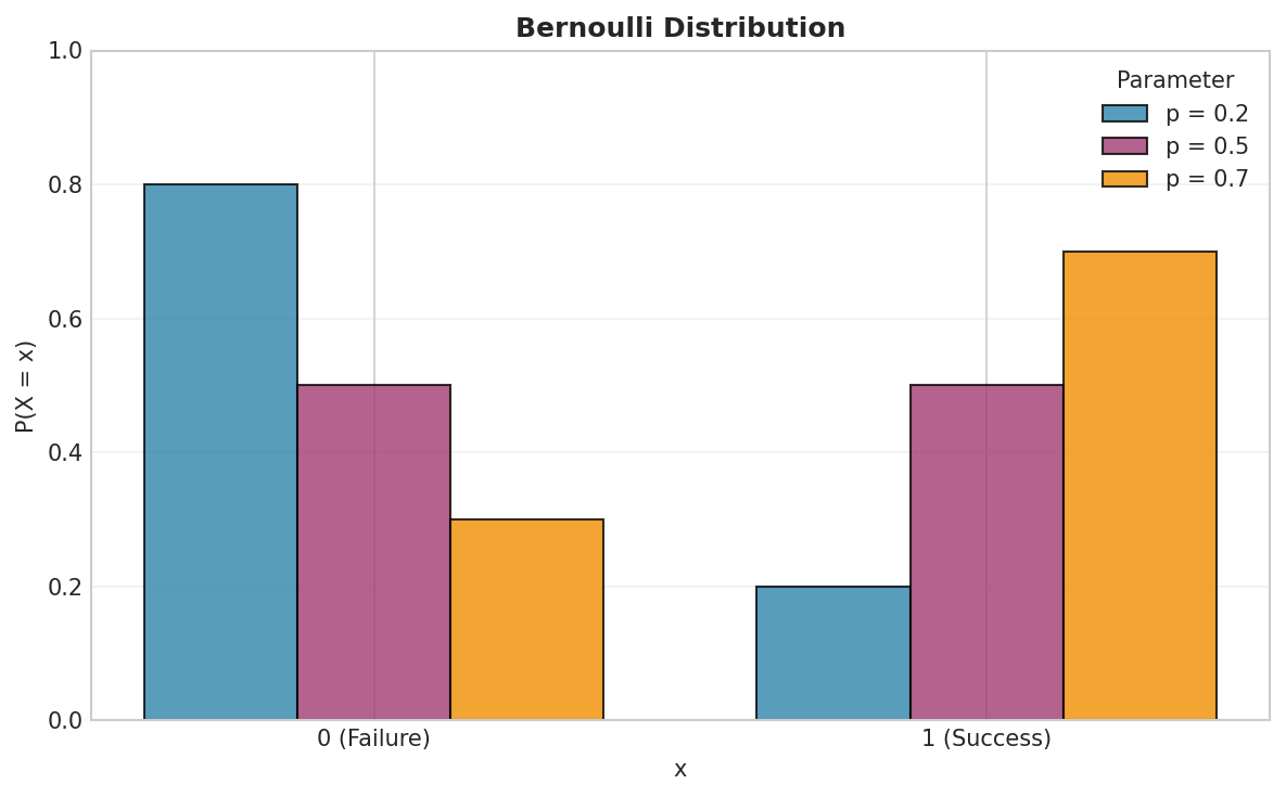
Fig. 8 The Bernoulli distribution is the simplest discrete distribution, modeling a single binary trial. As \(p\) increases, probability mass shifts from failure (0) to success (1).
Historical Context:
The Bernoulli distribution is named after Jacob Bernoulli (1654-1705), a Swiss mathematician from the famous Bernoulli family of scientists. His groundbreaking work “Ars Conjectandi” (The Art of Conjecturing), published posthumously in 1713, established probability theory as a mathematical discipline. In this work, Bernoulli proved the first version of the law of large numbers, showing that as the number of trials increases, the observed frequency of success converges to the true probability. This was revolutionary—it provided a mathematical bridge between theoretical probability and observed frequencies, laying the foundation for statistical inference.
Properties:
Mean: \(E[X] = p\)
Variance: \(\text{Var}(X) = p(1-p)\)
Moment Generating Function: \(M_X(t) = (1-p) + pe^t\)
Support: \(\{0, 1\}\)
Derivation: Mean and Variance
Mean:
Variance:
Let’s explore this distribution computationally:
def bernoulli_exploration(p=0.3, n_trials=1000):
    """Explore Bernoulli distribution through multiple methods."""

    # Method 1: Using random module
    successes_random = sum(1 for _ in range(n_trials) if random.random() < p)

    # Method 2: Using NumPy (vectorized)
    successes_numpy = np.sum(np.random.random(n_trials) < p)

    # Method 3: Using NumPy's binomial with n=1
    successes_binom = np.sum(np.random.binomial(1, p, n_trials))

    # Method 4: Using SciPy for exact probabilities
    bernoulli_dist = stats.bernoulli(p)

    print(f"Bernoulli Distribution with p = {p}")
    print(f"Theoretical mean: {p}")
    print(f"Theoretical variance: {p*(1-p):.3f}")
    print(f"Simulated mean (random): {successes_random/n_trials:.3f}")
    print(f"Simulated mean (numpy): {successes_numpy/n_trials:.3f}")
    print(f"\nExact probabilities:")
    print(f"P(X=0) = {bernoulli_dist.pmf(0):.3f}")
    print(f"P(X=1) = {bernoulli_dist.pmf(1):.3f}")

# Run the exploration
bernoulli_exploration(p=0.7)
Now let’s visualize the convergence to the true probability:
# Visualize convergence - Law of Large Numbers
def plot_bernoulli_convergence(p=0.7, n_trials=1000):
    # Generate a sequence of trials
    trials = np.random.binomial(1, p, n_trials)

    # Running mean
    running_mean = np.cumsum(trials) / np.arange(1, n_trials + 1)

    plt.figure(figsize=(10, 6))
    plt.plot(running_mean, alpha=0.8, linewidth=2)
    plt.axhline(y=p, color='r', linestyle='--', label=f'True mean = {p}')
    plt.xlabel('Number of trials')
    plt.ylabel('Running mean')
    plt.title('Law of Large Numbers: Bernoulli Distribution')
    plt.legend()
    plt.grid(True, alpha=0.3)
    plt.show()

plot_bernoulli_convergence()
Binomial Distribution
Definition
The Binomial distribution models the number of successes in \(n\) independent Bernoulli trials, each with success probability \(p\).
Parameterization: Binomial(n = number of trials, p = success probability)
A random variable \(X \sim \text{Binomial}(n, p)\) has probability mass function:
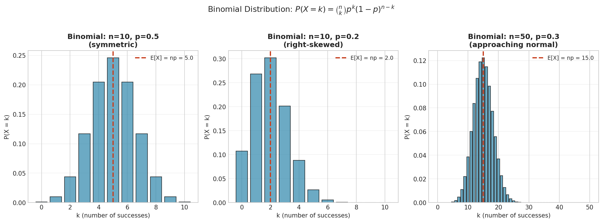
Fig. 9 Binomial distribution shapes. Left: Binomial(10, 0.5) is symmetric around the mean \(np = 5\). Center: Binomial(10, 0.2) is right-skewed when \(p < 0.5\). Right: Binomial(50, 0.3) approaches a normal distribution as \(n\) grows large (CLT).
Historical Context:
The binomial distribution’s history is intertwined with the development of probability theory itself. Jacob Bernoulli studied it extensively in the late 1600s, but it was Abraham de Moivre who made the breakthrough connection to the normal distribution. In 1733, de Moivre showed that for large n, the binomial distribution could be approximated by what we now call the normal distribution. This was one of the first limit theorems in probability, predating the formal central limit theorem by nearly two centuries. The approximation was crucial for practical calculations in an era before computers—computing binomial probabilities for large n was computationally intractable.
Properties:
Mean: \(E[X] = np\)
Variance: \(\text{Var}(X) = np(1-p)\)
Moment Generating Function: \(M_X(t) = [(1-p) + pe^t]^n\)
Support: \(\{0, 1, 2, ..., n\}\)
Theorem: Sum of Bernoulli Trials
If \(X_1, X_2, ..., X_n\) are independent \(\text{Bernoulli}(p)\) random variables, then:
Proof: Using moment generating functions:
This is the MGF of \(\text{Binomial}(n, p)\), proving the result.
Theorem: Normal Approximation (De Moivre-Laplace)
For \(X \sim \text{Binomial}(n, p)\), as \(n \to \infty\):
Proof:
Write \(X = \sum_{i=1}^n X_i\) where \(X_i \sim \text{Bernoulli}(p)\)
Each \(X_i\) has mean \(\mu = p\) and variance \(\sigma^2 = p(1-p)\)
By the Central Limit Theorem:
\[\frac{\sum_{i=1}^n X_i - n\mu}{\sigma\sqrt{n}} = \frac{X - np}{\sqrt{np(1-p)}} \xrightarrow{d} \mathcal{N}(0, 1)\]
The binomial distribution implementation:
def binomial_calculations(n=20, p=0.3):
    """Demonstrate binomial distribution calculations."""

    # Generate samples
    samples = np.random.binomial(n, p, 10000)

    # Theoretical moments
    mean_theory = n * p
    var_theory = n * p * (1 - p)

    print(f"Binomial({n}, {p}) Properties:")
    print(f"Theoretical mean: {mean_theory}")
    print(f"Empirical mean: {np.mean(samples):.2f}")
    print(f"Theoretical variance: {var_theory:.2f}")
    print(f"Empirical variance: {np.var(samples):.2f}")

    # Calculate some probabilities
    k_values = range(0, n+1)
    pmf_values = stats.binom.pmf(k_values, n, p)

    # Find mode
    mode = int((n + 1) * p)
    if (n + 1) * p == mode:  # Check if there are two modes
        print(f"Modes: {mode-1} and {mode}")
    else:
        print(f"Mode: {mode}")

    return samples, pmf_values

samples, pmf_values = binomial_calculations()
Visualizing the normal approximation:
def plot_normal_approximation(n=100, p=0.3):
    """Demonstrate the De Moivre-Laplace theorem."""

    # Binomial distribution
    x_binom = np.arange(0, n+1)
    pmf_binom = stats.binom.pmf(x_binom, n, p)

    # Normal approximation parameters
    mu = n * p
    sigma = np.sqrt(n * p * (1 - p))

    # For continuous approximation
    x_norm = np.linspace(0, n, 1000)
    pdf_norm = stats.norm.pdf(x_norm, mu, sigma)

    plt.figure(figsize=(12, 6))

    # Subplot 1: Direct comparison
    plt.subplot(1, 2, 1)
    plt.bar(x_binom, pmf_binom, alpha=0.5, label='Binomial', width=1.0)
    plt.plot(x_norm, pdf_norm, 'r-', linewidth=2,
             label='Normal approximation')

    plt.xlabel('Number of successes')
    plt.ylabel('Probability/Density')
    plt.title(f'Binomial({n}, {p}) vs Normal({mu:.1f}, {sigma:.1f}²)')
    plt.legend()
    plt.xlim(mu - 4*sigma, mu + 4*sigma)
    plt.grid(True, alpha=0.3)

    # Subplot 2: Standardized comparison
    plt.subplot(1, 2, 2)
    x_standard = (x_binom - mu) / sigma
    plt.bar(x_standard, pmf_binom * sigma, alpha=0.5,
            label='Standardized Binomial', width=1/sigma)

    z = np.linspace(-4, 4, 1000)
    plt.plot(z, stats.norm.pdf(z), 'r-', linewidth=2,
             label='Standard Normal')

    plt.xlabel('Standardized value')
    plt.ylabel('Density')
    plt.title('Standardized Comparison')
    plt.legend()
    plt.xlim(-4, 4)
    plt.grid(True, alpha=0.3)

    plt.tight_layout()
    plt.show()

plot_normal_approximation()
Poisson Distribution
Definition
The Poisson distribution models the number of events occurring in a fixed interval of time or space, given a constant average rate \(\lambda\).
Parameterization: Poisson(λ = average rate of events)
A random variable \(X \sim \text{Poisson}(\lambda)\) has probability mass function:
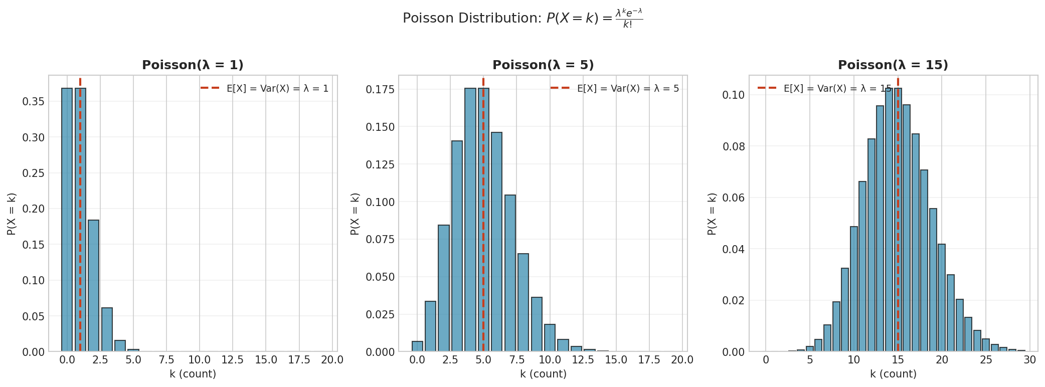
Fig. 10 Poisson distribution for different rates. As \(\lambda\) increases, the distribution shifts rightward and becomes more symmetric. Note that \(E[X] = Var(X) = \lambda\)—a defining characteristic used to identify Poisson-distributed count data.
Historical Context:
Siméon Denis Poisson introduced this distribution in 1837 while studying the probability of wrongful convictions in French courts. He was interested in modeling rare events—specifically, the chance that a given jury would convict an innocent person. The distribution gained practical prominence through Ladislaus Bortkiewicz’s famous 1898 analysis of deaths by horse kicks in the Prussian cavalry. Over 20 years, 10 cavalry corps experienced 196 deaths, averaging 0.61 per corps per year. Bortkiewicz showed that the number of deaths per corps per year followed a Poisson distribution almost perfectly, demonstrating the distribution’s utility for modeling rare, random events.
Properties:
Mean: \(E[X] = \lambda\)
Variance: \(\text{Var}(X) = \lambda\) (mean equals variance!)
Moment Generating Function: \(M_X(t) = e^{\lambda(e^t - 1)}\)
Support: \(\{0, 1, 2, ...\}\)
Derivation: Mean Equals Variance Property
Mean:
Second Moment:
Theorem: Poisson Limit Theorem
Let \(X_n \sim \text{Binomial}(n, p_n)\) where \(p_n = \lambda/n\) for fixed \(\lambda > 0\). Then as \(n \to \infty\):
Proof:
As \(n \to \infty\): - \(\frac{n(n-1)...(n-k+1)}{n^k} \to 1\) - \(\left(1-\frac{\lambda}{n}\right)^n \to e^{-\lambda}\) - \(\left(1-\frac{\lambda}{n}\right)^{-k} \to 1\)
Therefore: \(P(X_n = k) \to \frac{\lambda^k e^{-\lambda}}{k!}\), which is the probability mass function of Poisson(\(\lambda\)).
Let’s explore the Poisson distribution:
def poisson_mean_variance_property(lambda_param=4):
    """Demonstrate that mean equals variance for Poisson."""

    # Generate samples
    samples = np.random.poisson(lambda_param, 10000)

    print(f"Poisson({lambda_param}) Mean = Variance Property:")
    print(f"Theoretical mean = variance = {lambda_param}")
    print(f"Empirical mean: {np.mean(samples):.3f}")
    print(f"Empirical variance: {np.var(samples):.3f}")
    print(f"Ratio variance/mean: {np.var(samples)/np.mean(samples):.3f}")

    # Calculate index of dispersion
    dispersion = np.var(samples) / np.mean(samples)
    print(f"Index of dispersion: {dispersion:.3f} (should be ≈ 1)")

poisson_mean_variance_property()
Demonstrating the Poisson limit theorem:
def plot_poisson_limit_theorem(lam=5):
    """Show how Binomial converges to Poisson for rare events."""

    x = np.arange(0, 15)

    plt.figure(figsize=(10, 6))

    # Poisson distribution
    poisson_pmf = stats.poisson.pmf(x, lam)
    plt.plot(x, poisson_pmf, 'ko-', linewidth=2, markersize=8,
             label=f'Poisson({lam})')

    # Binomial approximations with increasing n
    for n in [20, 50, 100, 500]:
        p = lam / n
        binom_pmf = stats.binom.pmf(x, n, p)
        plt.plot(x, binom_pmf, 'o--', alpha=0.7, markersize=5,
                 label=f'Binomial({n}, {p:.4f})')

    plt.xlabel('k')
    plt.ylabel('P(X=k)')
    plt.title('Poisson Limit Theorem: Binomial → Poisson as n→∞, p→0, np→λ')
    plt.legend()
    plt.grid(True, alpha=0.3)
    plt.show()

plot_poisson_limit_theorem()
Connection to exponential distribution:
def plot_poisson_exponential_connection(lambda_rate=2, T=10):
    """Show connection between Poisson counts and exponential waiting times."""

    # Generate a Poisson process
    n_events = np.random.poisson(lambda_rate * T)

    # Method 1: Uniform arrival times
    arrival_times = np.sort(np.random.uniform(0, T, n_events))

    # Calculate inter-arrival times
    inter_arrivals = np.diff(np.concatenate([[0], arrival_times]))

    fig, (ax1, ax2) = plt.subplots(1, 2, figsize=(12, 5))

    # Plot 1: The process
    ax1.eventplot(arrival_times, colors='blue', linewidths=2)
    ax1.set_xlim(0, T)
    ax1.set_ylim(0.5, 1.5)
    ax1.set_xlabel('Time')
    ax1.set_title(f'Poisson Process (λ={lambda_rate} events/time unit)')
    ax1.set_yticks([])
    ax1.grid(True, alpha=0.3)

    # Plot 2: Inter-arrival distribution
    ax2.hist(inter_arrivals, bins=20, density=True, alpha=0.7,
             label='Inter-arrival times')

    x = np.linspace(0, max(inter_arrivals), 100)
    ax2.plot(x, lambda_rate * np.exp(-lambda_rate * x), 'r-',
             linewidth=2, label=f'Exponential(λ={lambda_rate})')

    ax2.set_xlabel('Time between events')
    ax2.set_ylabel('Density')
    ax2.set_title('Inter-arrival Times are Exponential')
    ax2.legend()
    ax2.grid(True, alpha=0.3)

    plt.tight_layout()
    plt.show()

plot_poisson_exponential_connection()
Geometric Distribution
Definition
The Geometric distribution models the number of trials needed to get the first success in a sequence of independent Bernoulli trials.
Parameterization: Geometric(p = probability of success per trial)
Important: Different sources use different conventions:
SciPy convention (used throughout this chapter): X = number of trials until first success, support {1, 2, 3, …}
Alternative convention: X = number of failures before first success, support {0, 1, 2, …}
Using SciPy’s convention, \(X \sim \text{Geometric}(p)\) has probability mass function:
Properties:
Mean: \(E[X] = \frac{1}{p}\) (average number of trials until success)
Variance: \(\text{Var}(X) = \frac{1-p}{p^2}\)
Moment Generating Function: \(M_X(t) = \frac{pe^t}{1-(1-p)e^t}\) for \(t < -\ln(1-p)\)
Memoryless property: \(P(X > s+t | X > s) = P(X > t)\)
Theorem: Memoryless Property
The geometric distribution is the only discrete distribution with the memoryless property:
Proof:
First, note that \(P(X > k) = (1-p)^k\) for \(k \geq 0\).
Derivation: Mean and Variance
Mean: Using the fact that \(\sum_{k=1}^{\infty} k x^{k-1} = \frac{1}{(1-x)^2}\) for \(|x| < 1\):
Variance: First compute \(E[X^2]\):
Demonstrating the memoryless property:
def demonstrate_memoryless_property(p=0.3):
    """Show the memoryless property of geometric distribution."""

    n_simulations = 100000
    samples = np.random.geometric(p, n_simulations)

    # Test memoryless property: P(X > s+t | X > s) = P(X > t)
    s, t = 5, 3

    # P(X > t)
    prob_greater_t = np.mean(samples > t)

    # P(X > s+t | X > s)
    samples_greater_s = samples[samples > s]
    prob_conditional = np.mean(samples_greater_s > s + t)

    # Theoretical value
    theoretical = (1 - p) ** t

    print(f"Memoryless Property Test (p={p}):")
    print(f"P(X > {t}) = {prob_greater_t:.4f}")
    print(f"P(X > {s+t} | X > {s}) = {prob_conditional:.4f}")
    print(f"Theoretical value: {theoretical:.4f}")
    print(f"\nInterpretation: Past failures don't affect future probability!")
    print(f"Having already waited {s} trials doesn't change the probability")
    print(f"of waiting {t} more trials.")

demonstrate_memoryless_property()
Expected waiting time visualization:
def plot_geometric_analysis(p=0.2):
    """Comprehensive analysis of geometric distribution."""

    fig, ((ax1, ax2), (ax3, ax4)) = plt.subplots(2, 2, figsize=(12, 10))

    # PMF for different p values
    x = np.arange(1, 21)
    for p_val in [0.1, 0.3, 0.5, 0.7]:
        pmf = stats.geom.pmf(x, p_val)
        ax1.plot(x, pmf, 'o-', label=f'p={p_val}', markersize=6)

    ax1.set_xlabel('Number of trials until first success')
    ax1.set_ylabel('Probability')
    ax1.set_title('Geometric Distribution PMF')
    ax1.legend()
    ax1.grid(True, alpha=0.3)

    # Survival function (log scale)
    x_surv = np.arange(0, 50)
    for p_val in [0.1, 0.3, 0.5]:
        survival = (1 - p_val) ** x_surv
        ax2.semilogy(x_surv, survival, 'o-', label=f'p={p_val}', markersize=4)

    ax2.set_xlabel('k')
    ax2.set_ylabel('P(X > k)')
    ax2.set_title('Survival Function (Log Scale)')
    ax2.legend()
    ax2.grid(True, alpha=0.3)

    # Convergence to expected value
    n_samples = 1000
    samples = np.random.geometric(p, n_samples)
    running_mean = np.cumsum(samples) / np.arange(1, n_samples + 1)

    ax3.plot(running_mean, alpha=0.8, linewidth=2)
    ax3.axhline(y=1/p, color='red', linestyle='--',
                label=f'Expected value = 1/p = {1/p:.1f}')
    ax3.set_xlabel('Number of experiments')
    ax3.set_ylabel('Average trials until first success')
    ax3.set_title(f'Convergence to Expected Waiting Time (p={p})')
    ax3.legend()
    ax3.grid(True, alpha=0.3)

    # Memoryless property visualization
    trials = 100
    paths = 20
    for i in range(paths):
        wait_times = []
        current_pos = 0
        while current_pos < trials:
            wait = np.random.geometric(p)
            current_pos += wait
            wait_times.append(current_pos)
        ax4.plot(wait_times, range(len(wait_times)), 'o-', alpha=0.3, markersize=3)

    ax4.set_xlabel('Trial number')
    ax4.set_ylabel('Number of successes')
    ax4.set_title(f'Sample Paths (p={p})')
    ax4.grid(True, alpha=0.3)

    plt.tight_layout()
    plt.show()

plot_geometric_analysis()
Negative Binomial Distribution
Definition
The Negative Binomial distribution models the number of failures before the \(r\)-th success in a sequence of independent Bernoulli trials.
Parameterization: NegativeBinomial(r = target number of successes, p = success probability per trial)
Output: Number of failures before achieving r successes
A random variable \(X \sim \text{NegBinomial}(r, p)\) has probability mass function:
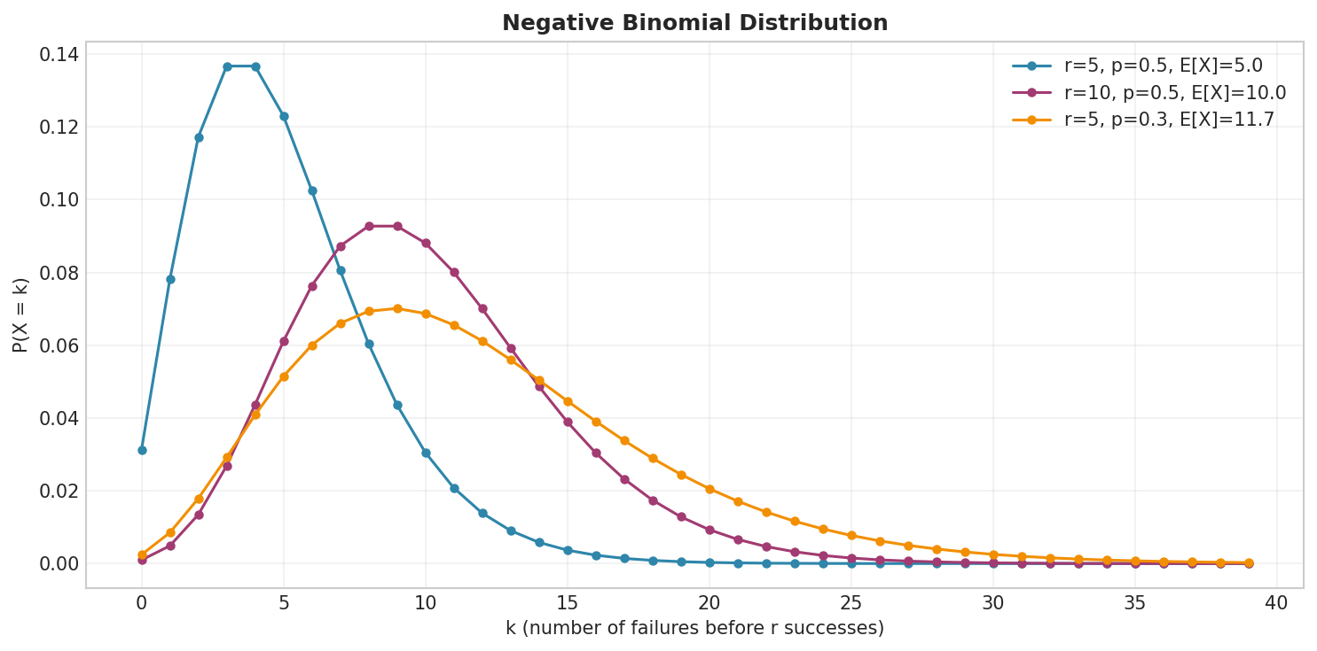
Fig. 11 Negative Binomial distribution models the number of failures before \(r\) successes. Increasing \(r\) shifts and spreads the distribution; decreasing \(p\) increases the expected number of failures.
Alternative Interpretation: The Negative Binomial can also be viewed as a Poisson distribution where the rate parameter itself follows a Gamma distribution (Gamma-Poisson mixture). This makes it excellent for modeling overdispersed count data.
Properties:
Mean: \(E[X] = \frac{r(1-p)}{p}\) (average number of failures before r successes)
Variance: \(\text{Var}(X) = \frac{r(1-p)}{p^2}\)
Moment Generating Function: \(M_X(t) = \left(\frac{p}{1-(1-p)e^t}\right)^r\) for \(t < -\ln(1-p)\)
Overdispersion: Variance > Mean (unlike Poisson where Variance = Mean)
Theorem: Sum of Geometric Random Variables
If \(Y_1, Y_2, ..., Y_r\) are independent \(\text{Geometric}(p)\) random variables (number of trials until success, SciPy convention), then:
where \(X\) represents the number of failures before the \(r\)-th success.
Proof: The \(r\)-th success occurs after \(\sum Y_i\) total trials, which includes \(r\) successes and \(X = \sum Y_i - r\) failures.
Note: With SciPy’s convention, if \(Y \sim \text{Geometric}(p)\) and \(X \sim \text{NegBinomial}(1, p)\), then \(Y = X + 1\) (since Geometric counts trials, NegBinomial counts failures).
Relationship: Gamma-Poisson Mixture
If \(\Lambda \sim \text{Gamma}(\alpha, \beta)\) and \(X|\Lambda \sim \text{Poisson}(\Lambda)\), then marginally:
This explains why the negative binomial models overdispersed count data.
Let’s explore the negative binomial:
def demonstrate_overdispersion():
    """Compare Poisson and Negative Binomial for overdispersed data."""

    mean_val = 10

    # Poisson with same mean
    poisson_samples = np.random.poisson(mean_val, 10000)

    # Negative Binomial with same mean but higher variance
    r = 5
    p = r / (r + mean_val)  # This gives mean = r(1-p)/p = 10
    nbinom_samples = stats.nbinom.rvs(r, p, size=10000)

    print("Overdispersion Comparison:")
    print(f"Target mean: {mean_val}")
    print(f"\nPoisson (mean = variance):")
    print(f"  Sample mean: {np.mean(poisson_samples):.2f}")
    print(f"  Sample variance: {np.var(poisson_samples):.2f}")
    print(f"  Variance/Mean ratio: {np.var(poisson_samples)/np.mean(poisson_samples):.2f}")
    print(f"\nNegative Binomial (overdispersed):")
    print(f"  Sample mean: {np.mean(nbinom_samples):.2f}")
    print(f"  Sample variance: {np.var(nbinom_samples):.2f}")
    print(f"  Variance/Mean ratio: {np.var(nbinom_samples)/np.mean(nbinom_samples):.2f}")

    # Theoretical variance for negative binomial
    var_theory = r * (1 - p) / p**2
    print(f"\n  Theoretical variance: {var_theory:.2f}")

demonstrate_overdispersion()
Demonstrating the sum of geometrics relationship:
def show_nbinom_as_sum_of_geometric():
    """Show that Negative Binomial is sum of Geometric random variables."""

    r = 5  # number of successes
    p = 0.3  # success probability
    n_simulations = 10000

    # Method 1: Sum of geometric distributions
    failures_from_geometric = []
    for _ in range(n_simulations):
        total_trials = sum(np.random.geometric(p) for _ in range(r))
        failures = total_trials - r
        failures_from_geometric.append(failures)

    # Method 2: Direct negative binomial
    nbinom_direct = stats.nbinom.rvs(r, p, size=n_simulations)

    fig, (ax1, ax2) = plt.subplots(1, 2, figsize=(12, 5))

    # Histogram comparison
    bins = np.arange(0, max(max(failures_from_geometric), max(nbinom_direct)) + 1)
    ax1.hist(failures_from_geometric, bins=bins, density=True, alpha=0.5,
             label='Sum of Geometric - r')
    ax1.hist(nbinom_direct, bins=bins, density=True, alpha=0.5,
             label='Direct Negative Binomial')

    # Theoretical PMF
    x = np.arange(0, 40)
    pmf = stats.nbinom.pmf(x, r, p)
    ax1.plot(x, pmf, 'r-', linewidth=2, label='Theoretical PMF')

    ax1.set_xlabel('Number of failures before r successes')
    ax1.set_ylabel('Density')
    ax1.set_title(f'Negative Binomial as Sum of Geometric (r={r}, p={p})')
    ax1.legend()
    ax1.grid(True, alpha=0.3)

    # QQ plot
    from scipy.stats import probplot
    probplot(failures_from_geometric, dist=stats.nbinom(r, p), plot=ax2)
    ax2.set_title('Q-Q Plot: Sum of Geometric vs NegBinom Theory')
    ax2.grid(True, alpha=0.3)

    plt.tight_layout()
    plt.show()

show_nbinom_as_sum_of_geometric()
Continuous Distributions
Continuous probability distributions model random variables that can take any value within a continuous range. These distributions are fundamental for modeling measurements, time intervals, and other continuous phenomena.
Uniform Distribution
Definition
The Uniform distribution assigns equal probability to all values in an interval [a, b].
Parameterization: Uniform(a = lower bound, b = upper bound)
A random variable \(X \sim \text{Uniform}(a, b)\) has probability density function:
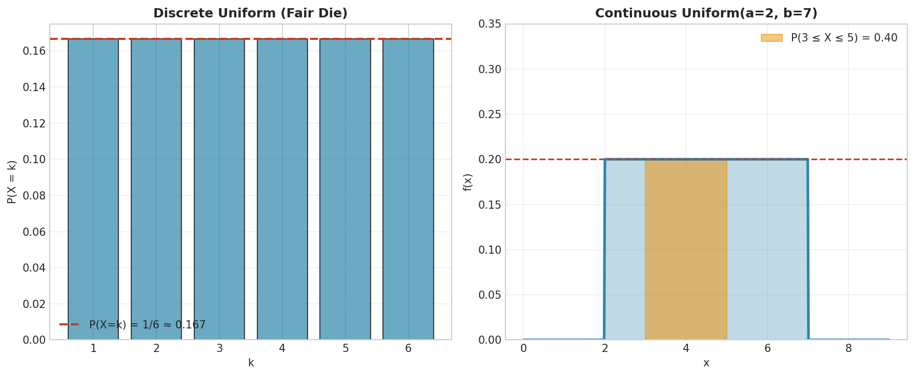
Fig. 12 Uniform distributions. Left: Discrete uniform on {1, 2, 3, 4, 5, 6} (fair die)—each outcome has equal probability 1/6. Right: Continuous Uniform(2, 7) with constant density \(f(x) = 0.2\); the shaded region shows \(P(3 \leq X \leq 5) = 0.4\).
Historical Context:
The uniform distribution is perhaps the most intuitive probability distribution, representing complete ignorance within known bounds. Its theoretical importance was recognized by Pierre-Simon Laplace, who used it as the foundation for his “principle of insufficient reason” (later called the principle of indifference): when we have no information favoring one outcome over another, we should assign equal probabilities. This principle, while philosophically controversial, makes the uniform distribution the starting point for many analyses. The principle of indifference can be traced back to Jacob Bernoulli’s “Ars Conjectandi” (1713), though Laplace formalized and popularized it. The uniform distribution also serves as the foundation for random number generation—most pseudo-random number generators produce uniform(0,1) values that are then transformed to other distributions.
Properties:
Mean: \(E[X] = \frac{a+b}{2}\)
Variance: \(\text{Var}(X) = \frac{(b-a)^2}{12}\)
Moment Generating Function: \(M_X(t) = \frac{e^{tb} - e^{ta}}{t(b-a)}\) for \(t \neq 0\)
Standard uniform: When \(a = 0, b = 1\), used for random number generation
Derivation: Mean and Variance
Mean:
Variance:
Theorem: Probability Integral Transform
If \(X\) is a continuous random variable with CDF \(F_X\), then:
Conversely, if \(U \sim \text{Uniform}(0, 1)\) and \(F\) is a CDF, then:
Proof of first part: For \(u \in [0, 1]\):
This is the CDF of Uniform(0, 1).
Let’s explore the uniform distribution:
def explore_uniform_properties():
    """Comprehensive exploration of uniform distribution."""

    a, b = -3.0, 2.0
    n = 10000

    # Generate samples
    samples = np.random.uniform(a, b, n)

    # Theoretical values
    theo_mean = 0.5 * (a + b)
    theo_var = (b - a)**2 / 12
    theo_median = (a + b) / 2

    print(f"Uniform({a}, {b}) Properties:")
    print(f"Theoretical mean: {theo_mean:.4f}")
    print(f"Empirical mean: {np.mean(samples):.4f}")
    print(f"Theoretical variance: {theo_var:.4f}")
    print(f"Empirical variance: {np.var(samples):.4f}")
    print(f"Theoretical median: {theo_median:.4f}")
    print(f"Empirical median: {np.median(samples):.4f}")

    # Test uniformity
    bins = 20
    counts, edges = np.histogram(samples, bins=bins, range=(a, b))
    expected_count = n / bins
    chi2_stat = np.sum((counts - expected_count)**2 / expected_count)

    print(f"\nUniformity test (Chi-square):")
    print(f"Chi-square statistic: {chi2_stat:.2f}")
    print(f"Critical value (α=0.05, df={bins-1}): {stats.chi2.ppf(0.95, bins-1):.2f}")

explore_uniform_properties()
Demonstrating the probability integral transform:
def demonstrate_probability_integral_transform():
    """Show the probability integral transform in action."""

    n = 10000

    # Start with exponential random variables
    lambda_param = 2.0
    exp_samples = np.random.exponential(1/lambda_param, n)

    # Apply the CDF to get uniform
    uniform_transformed = 1 - np.exp(-lambda_param * exp_samples)

    # Generate uniform and transform to exponential
    uniform_samples = np.random.uniform(0, 1, n)
    exp_transformed = -np.log(1 - uniform_samples) / lambda_param

    fig, ((ax1, ax2), (ax3, ax4)) = plt.subplots(2, 2, figsize=(12, 10))

    # Original exponential
    ax1.hist(exp_samples, bins=50, density=True, alpha=0.7,
             label='Original Exponential')
    x = np.linspace(0, max(exp_samples), 100)
    ax1.plot(x, lambda_param * np.exp(-lambda_param * x), 'r-',
             linewidth=2, label='Theory')
    ax1.set_xlabel('Value')
    ax1.set_ylabel('Density')
    ax1.set_title('Original Exponential Distribution')
    ax1.legend()
    ax1.grid(True, alpha=0.3)

    # Transformed to uniform
    ax2.hist(uniform_transformed, bins=50, density=True, alpha=0.7,
             label='F(X) where X ~ Exp')
    ax2.axhline(y=1, color='r', linestyle='--', linewidth=2,
                label='Uniform(0,1)')
    ax2.set_xlabel('Value')
    ax2.set_ylabel('Density')
    ax2.set_title('CDF Transform → Uniform')
    ax2.legend()
    ax2.grid(True, alpha=0.3)

    # Original uniform
    ax3.hist(uniform_samples, bins=50, density=True, alpha=0.7,
             label='Original Uniform')
    ax3.axhline(y=1, color='r', linestyle='--', linewidth=2,
                label='Theory')
    ax3.set_xlabel('Value')
    ax3.set_ylabel('Density')
    ax3.set_title('Original Uniform Distribution')
    ax3.legend()
    ax3.grid(True, alpha=0.3)

    # Transformed to exponential
    ax4.hist(exp_transformed, bins=50, density=True, alpha=0.7,
             label='F⁻¹(U) where U ~ Unif')
    x = np.linspace(0, max(exp_transformed), 100)
    ax4.plot(x, lambda_param * np.exp(-lambda_param * x), 'r-',
             linewidth=2, label='Exponential')
    ax4.set_xlabel('Value')
    ax4.set_ylabel('Density')
    ax4.set_title('Inverse CDF Transform → Exponential')
    ax4.legend()
    ax4.grid(True, alpha=0.3)

    plt.tight_layout()
    plt.show()

demonstrate_probability_integral_transform()
Normal (Gaussian) Distribution
Definition
The Normal distribution is characterized by its bell-shaped curve and is defined by two parameters.
Parameterization: Normal(μ = mean, σ² = variance) or Normal(μ = mean, σ = standard deviation)
A random variable \(X \sim \mathcal{N}(\mu, \sigma^2)\) has probability density function:
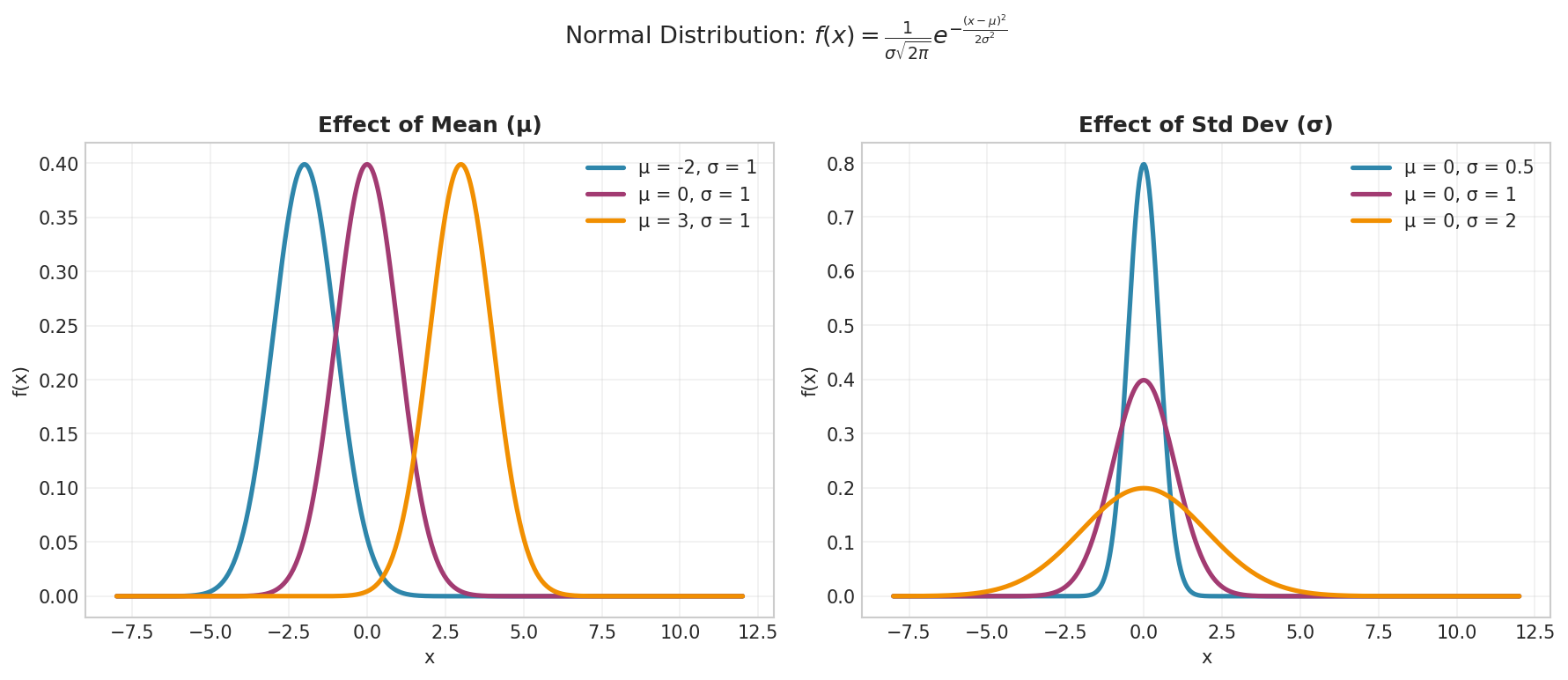
Fig. 13 Normal distribution parameter effects. Left: Changing \(\mu\) shifts the distribution along the x-axis without affecting shape. Right: Changing \(\sigma\) controls spread—smaller \(\sigma\) produces a taller, narrower curve; larger \(\sigma\) produces a flatter, wider curve.
Historical Context:
The normal distribution has a rich history involving multiple independent discoveries. Abraham de Moivre first derived it in 1733 as an approximation to the binomial distribution. Pierre-Simon Laplace extended this work, developing what we now call the Central Limit Theorem. However, the distribution bears Carl Friedrich Gauss’s name because of his 1809 work on astronomical measurement errors. Gauss showed that if errors are due to many small, independent causes, they follow this distribution—hence “Gaussian distribution.” The term “normal” was popularized by Francis Galton, who viewed it as the natural state of variation. Today, we know the normal distribution emerges whenever many independent factors contribute additively to an outcome, making it ubiquitous in nature and statistics.
Properties:
Mean: \(E[X] = \mu\)
Variance: \(\text{Var}(X) = \sigma^2\)
Moment Generating Function: \(M_X(t) = \exp(\mu t + \frac{\sigma^2 t^2}{2})\)
Support: \((-\infty, \infty)\)
Symmetry: Symmetric about the mean
68-95-99.7 Rule: Approximately 68%, 95%, and 99.7% of values lie within 1, 2, and 3 standard deviations of the mean
Theorem: Central Limit Theorem
Let \(X_1, X_2, ..., X_n\) be independent and identically distributed random variables with mean \(\mu\) and variance \(\sigma^2 < \infty\). Then:
where \(\bar{X}_n = \frac{1}{n}\sum_{i=1}^n X_i\) is the sample mean.
Proof Sketch (using characteristic functions):
Let \(Y_i = \frac{X_i - \mu}{\sigma}\) (standardized)
The characteristic function of \(Y_i\) is \(\phi_Y(t) = 1 - \frac{t^2}{2} + o(t^2)\)
For \(S_n = \frac{\sum Y_i}{\sqrt{n}}\), we have \(\phi_{S_n}(t) = \left[\phi_Y(t/\sqrt{n})\right]^n\)
As \(n \to \infty\): \(\phi_{S_n}(t) \to e^{-t^2/2}\), which is the characteristic function of \(\mathcal{N}(0,1)\)
Derivation: 68-95-99.7 Rule
For \(Z \sim \mathcal{N}(0, 1)\):
For general \(X \sim \mathcal{N}(\mu, \sigma^2)\), use \(Z = (X - \mu)/\sigma\).
Let’s explore the normal distribution:
def explore_normal_properties(mu=0, sigma=1):
    """Comprehensive exploration of normal distribution."""

    # Generate samples
    n = 100000
    samples = np.random.normal(mu, sigma, n)

    print(f"Normal({mu}, {sigma}²) Properties:")
    print(f"Theoretical mean: {mu}")
    print(f"Empirical mean: {np.mean(samples):.4f}")
    print(f"Theoretical std: {sigma}")
    print(f"Empirical std: {np.std(samples):.4f}")

    # Check 68-95-99.7 rule
    within_1sigma = np.mean(np.abs(samples - mu) <= sigma)
    within_2sigma = np.mean(np.abs(samples - mu) <= 2*sigma)
    within_3sigma = np.mean(np.abs(samples - mu) <= 3*sigma)

    print(f"\n68-95-99.7 Rule:")
    print(f"Within 1σ: {within_1sigma:.1%} (theory: 68.3%)")
    print(f"Within 2σ: {within_2sigma:.1%} (theory: 95.4%)")
    print(f"Within 3σ: {within_3sigma:.1%} (theory: 99.7%)")

    # Compute higher moments
    standardized = (samples - mu) / sigma
    skewness = np.mean(standardized**3)
    kurtosis = np.mean(standardized**4)

    print(f"\nHigher moments (standardized):")
    print(f"Skewness: {skewness:.4f} (theory: 0)")
    print(f"Excess kurtosis: {kurtosis - 3:.4f} (theory: 0)")

explore_normal_properties(mu=100, sigma=15)
Demonstrating the Central Limit Theorem:
def demonstrate_clt():
    """Show CLT with various starting distributions."""

    n_samples = 10000
    sample_sizes = [1, 2, 5, 30]

    fig, axes = plt.subplots(2, 2, figsize=(12, 10))

    # Different starting distributions
    distributions = [
        ('Exponential', lambda n: np.random.exponential(1, n), 1, 1),
        ('Uniform', lambda n: np.random.uniform(0, 1, n), 0.5, 1/12),
        ('Chi-square', lambda n: np.random.chisquare(3, n), 3, 6),
        ('Beta', lambda n: np.random.beta(2, 5, n), 2/7, 10/343)
    ]

    for idx, (name, generator, true_mean, true_var) in enumerate(distributions):
        ax = axes[idx // 2, idx % 2]

        for n in sample_sizes:
            # Generate sample means
            sample_means = []
            for _ in range(n_samples):
                sample = generator(n)
                sample_means.append(np.mean(sample))

            # Standardize
            sample_means = np.array(sample_means)
            standardized = (sample_means - true_mean) / np.sqrt(true_var / n)

            # Plot histogram
            ax.hist(standardized, bins=50, density=True, alpha=0.5,
                    label=f'n={n}')

        # Overlay standard normal
        x = np.linspace(-4, 4, 100)
        ax.plot(x, stats.norm.pdf(x), 'k-', linewidth=2, label='N(0,1)')

        ax.set_xlabel('Standardized Sample Mean')
        ax.set_ylabel('Density')
        ax.set_title(f'CLT: {name} Distribution')
        ax.legend()
        ax.set_xlim(-4, 4)
        ax.grid(True, alpha=0.3)

    plt.tight_layout()
    plt.suptitle('Central Limit Theorem with Different Starting Distributions',
                 y=1.02, fontsize=14)
    plt.show()

demonstrate_clt()
Sum of normal random variables:
def demonstrate_normal_sum_property():
    """Show that sum of independent normals is normal."""

    # Parameters
    mu1, sigma1 = 2, 1
    mu2, sigma2 = -1, 2
    n = 10000

    # Generate independent normals
    X1 = np.random.normal(mu1, sigma1, n)
    X2 = np.random.normal(mu2, sigma2, n)

    # Sum
    X_sum = X1 + X2

    # Theoretical parameters of sum
    mu_sum = mu1 + mu2
    sigma_sum = np.sqrt(sigma1**2 + sigma2**2)

    plt.figure(figsize=(10, 6))

    # Plot empirical distribution
    plt.hist(X_sum, bins=50, density=True, alpha=0.7,
             label='X₁ + X₂ (empirical)')

    # Plot theoretical distribution
    x = np.linspace(mu_sum - 4*sigma_sum, mu_sum + 4*sigma_sum, 1000)
    pdf = stats.norm.pdf(x, mu_sum, sigma_sum)
    plt.plot(x, pdf, 'r-', linewidth=2,
             label=f'N({mu_sum}, {sigma_sum:.2f}²) (theory)')

    plt.xlabel('Value')
    plt.ylabel('Density')
    plt.title('Sum of Independent Normal Random Variables')
    plt.legend()
    plt.grid(True, alpha=0.3)

    print(f"X₁ ~ N({mu1}, {sigma1}²), X₂ ~ N({mu2}, {sigma2}²)")
    print(f"X₁ + X₂ ~ N({mu_sum}, {sigma_sum:.2f}²)")
    print(f"Empirical mean: {np.mean(X_sum):.3f}")
    print(f"Empirical std: {np.std(X_sum):.3f}")

    plt.show()

demonstrate_normal_sum_property()
Exponential Distribution
Definition
The Exponential distribution models the time between events in a Poisson process, characterized by a constant hazard rate.
Parameterization: - Rate parameterization: Exponential(λ = rate), where λ > 0 - Scale parameterization: Exponential(scale = 1/λ)
Note: NumPy uses scale parameterization, SciPy supports both.
Using rate parameterization, \(X \sim \text{Exp}(\lambda)\) has probability density function:
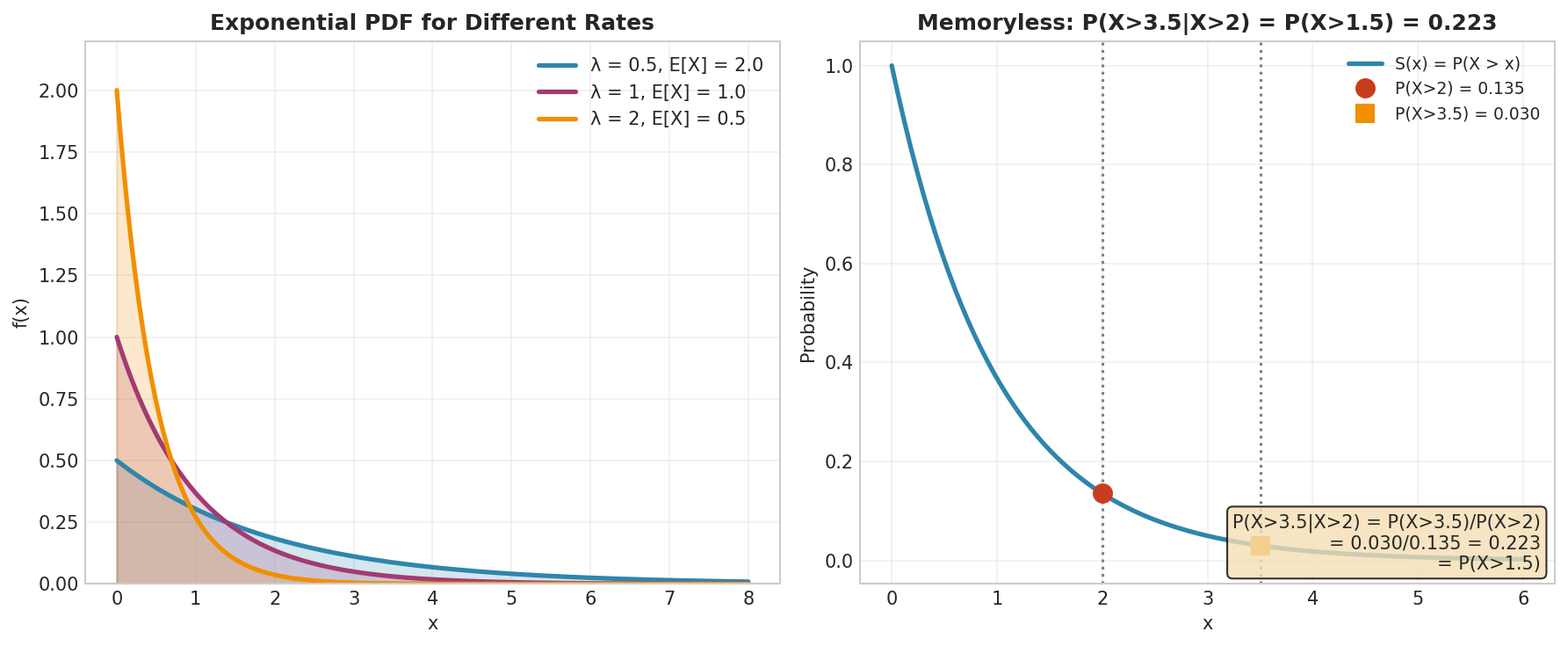
Fig. 14 Exponential distribution. Left: Higher rate \(\lambda\) means shorter expected waiting time (\(E[X] = 1/\lambda\)). Right: The memoryless property: \(P(X > s+t \mid X > s) = P(X > t)\). The conditional probability of surviving another \(t\) units is independent of how long you’ve already waited.
Historical Context:
The exponential distribution naturally arises from the Poisson process and was studied extensively in queueing theory by Agner Krarup Erlang in the early 1900s. Working for the Copenhagen Telephone Company, Erlang needed to determine how many telephone circuits were needed to provide acceptable service. He discovered that call durations followed an exponential distribution, and the time between calls also followed an exponential distribution. This work laid the foundation for queueing theory and operations research. The exponential distribution’s memoryless property made calculations tractable in an era before computers.
Properties:
Mean: \(E[X] = \frac{1}{\lambda}\)
Variance: \(\text{Var}(X) = \frac{1}{\lambda^2}\)
Moment Generating Function: \(M_X(t) = \frac{\lambda}{\lambda - t}\) for \(t < \lambda\)
Memoryless property: \(P(X > s + t | X > s) = P(X > t)\)
Relationship to Poisson: Inter-arrival times in a Poisson process
Minimum of exponentials: If \(X_i \sim \text{Exp}(\lambda_i)\), then \(\min(X_1, ..., X_n) \sim \text{Exp}(\sum \lambda_i)\)
Theorem: Memoryless Property
The exponential distribution is the only continuous distribution with the memoryless property:
Proof:
For \(X \sim \text{Exp}(\lambda)\), we have \(P(X > x) = e^{-\lambda x}\).
Converse: If \(P(X > s + t) = P(X > s)P(X > t)\) for all \(s, t > 0\), then setting \(g(x) = P(X > x)\):
This functional equation has solution \(g(x) = e^{-\lambda x}\), proving exponential is unique.
Derivation: Mean and Variance
Mean (using integration by parts):
Second Moment (using Gamma function):
Variance:
Let’s explore the exponential distribution:
def explore_exponential_basics(lam=2.0):
    """Basic properties of exponential distribution."""

    n = 10000

    # Note: NumPy uses scale parameter (1/λ), not rate
    samples_numpy = np.random.exponential(1/lam, n)

    # Using SciPy (which can use either parameterization)
    exp_dist = stats.expon(scale=1/lam)
    samples_scipy = exp_dist.rvs(n)

    print(f"Exponential({lam}) Properties:")
    print(f"Note: Using rate parameterization (λ={lam})")
    print(f"NumPy uses scale=1/λ={1/lam:.3f}")
    print(f"\nTheoretical mean: {1/lam:.4f}")
    print(f"Empirical mean: {np.mean(samples_numpy):.4f}")
    print(f"Theoretical std: {1/lam:.4f}")
    print(f"Empirical std: {np.std(samples_numpy):.4f}")

    # Verify variance = mean²
    print(f"\nMean² = {(1/lam)**2:.4f}")
    print(f"Variance = {np.var(samples_numpy):.4f}")

explore_exponential_basics()
Demonstrating the memoryless property:
def demonstrate_exponential_memoryless(lam=2.0):
    """Show the memoryless property of exponential distribution."""

    n = 100000
    samples = np.random.exponential(1/lam, n)

    # Test memoryless property at different values
    test_cases = [(1.0, 0.5), (2.0, 1.0), (0.5, 1.5)]

    print(f"Memoryless Property Test (λ={lam}):")
    print("-" * 60)

    for s, t in test_cases:
        # P(X > t)
        prob_greater_t = np.mean(samples > t)

        # P(X > s+t | X > s)
        samples_greater_s = samples[samples > s]
        if len(samples_greater_s) > 0:
            prob_conditional = np.mean(samples_greater_s > s + t)
        else:
            prob_conditional = 0

        # Theoretical value
        theoretical = np.exp(-lam * t)

        print(f"s={s}, t={t}:")
        print(f"  P(X > {t}) = {prob_greater_t:.4f}")
        print(f"  P(X > {s+t} | X > {s}) = {prob_conditional:.4f}")
        print(f"  Theoretical value: {theoretical:.4f}")
        print()

demonstrate_exponential_memoryless()
Relationship between exponential and Poisson:
def demonstrate_exponential_poisson_relationship(lam=3.0, T=10):
    """Show how exponential relates to Poisson process."""

    # Generate exponential inter-arrival times
    inter_arrivals = []
    current_time = 0
    while current_time < T:
        inter_arrival = np.random.exponential(1/lam)
        current_time += inter_arrival
        if current_time < T:
            inter_arrivals.append(inter_arrival)

    arrival_times = np.cumsum(inter_arrivals)
    n_events = len(arrival_times)

    fig, ((ax1, ax2), (ax3, ax4)) = plt.subplots(2, 2, figsize=(12, 10))

    # Plot 1: The Poisson process
    ax1.eventplot(arrival_times, colors='blue', linewidths=2)
    ax1.set_xlim(0, T)
    ax1.set_ylim(0.5, 1.5)
    ax1.set_xlabel('Time')
    ax1.set_title(f'Poisson Process (λ={lam} events/unit)')
    ax1.set_yticks([])
    ax1.grid(True, alpha=0.3)
    ax1.text(0.02, 0.95, f'Total events: {n_events}',
             transform=ax1.transAxes, verticalalignment='top')

    # Plot 2: Inter-arrival distribution
    ax2.hist(inter_arrivals, bins=30, density=True, alpha=0.7,
             label='Observed inter-arrivals')

    x = np.linspace(0, max(inter_arrivals) if inter_arrivals else 1, 100)
    ax2.plot(x, lam * np.exp(-lam * x), 'r-', linewidth=2,
             label=f'Exponential(λ={lam})')

    ax2.set_xlabel('Time between events')
    ax2.set_ylabel('Density')
    ax2.set_title('Inter-arrival Times')
    ax2.legend()
    ax2.grid(True, alpha=0.3)

    # Plot 3: Counting process
    count_times = np.linspace(0, T, 1000)
    counts = [np.sum(arrival_times <= t) for t in count_times]

    ax3.plot(count_times, counts, 'b-', linewidth=2, label='N(t)')
    ax3.plot(count_times, lam * count_times, 'r--', linewidth=2,
             label=f'E[N(t)] = λt')

    ax3.set_xlabel('Time')
    ax3.set_ylabel('Number of events')
    ax3.set_title('Counting Process N(t)')
    ax3.legend()
    ax3.grid(True, alpha=0.3)

    # Plot 4: Test Poisson distribution at fixed time
    n_sim = 1000
    counts_at_T = []
    for _ in range(n_sim):
        times = []
        t = 0
        while t < T:
            t += np.random.exponential(1/lam)
            if t < T:
                times.append(t)
        counts_at_T.append(len(times))

    k_values = np.arange(0, max(counts_at_T) + 1)
    observed_freq = [counts_at_T.count(k) / n_sim for k in k_values]
    theoretical_pmf = stats.poisson.pmf(k_values, lam * T)

    ax4.bar(k_values - 0.2, observed_freq, width=0.4, alpha=0.7,
            label='Observed')
    ax4.bar(k_values + 0.2, theoretical_pmf, width=0.4, alpha=0.7,
            label=f'Poisson({lam * T})')

    ax4.set_xlabel(f'Number of events in [0, {T}]')
    ax4.set_ylabel('Probability')
    ax4.set_title('Distribution of N(T)')
    ax4.legend()
    ax4.grid(True, alpha=0.3, axis='y')

    plt.tight_layout()
    plt.show()

demonstrate_exponential_poisson_relationship()
Minimum of exponentials property:
def demonstrate_minimum_exponentials():
    """Show that minimum of exponentials is exponential."""

    # System with multiple components
    component_rates = [1.0, 0.5, 2.0]  # Different failure rates
    n_sim = 10000

    # Simulate system failures
    min_times = []
    first_component = []

    for _ in range(n_sim):
        component_times = [np.random.exponential(1/rate)
                          for rate in component_rates]
        min_time = min(component_times)
        min_times.append(min_time)
        first_component.append(np.argmin(component_times))

    # Theoretical: min ~ Exp(sum of rates)
    total_rate = sum(component_rates)

    fig, (ax1, ax2) = plt.subplots(1, 2, figsize=(12, 5))

    # Distribution of minimum
    ax1.hist(min_times, bins=50, density=True, alpha=0.7,
             label='Simulated minimum')

    x = np.linspace(0, 3, 1000)
    ax1.plot(x, total_rate * np.exp(-total_rate * x), 'r-', linewidth=2,
             label=f'Exponential(λ={total_rate:.1f})')

    ax1.set_xlabel('Time to first failure')
    ax1.set_ylabel('Density')
    ax1.set_title('Minimum of Independent Exponentials')
    ax1.legend()
    ax1.grid(True, alpha=0.3)

    # Which component fails first
    component_labels = [f'Component {i+1}\n(λ={rate})'
                       for i, rate in enumerate(component_rates)]
    failure_probs = np.array(component_rates) / total_rate

    ax2.bar(range(len(component_rates)),
            [first_component.count(i)/n_sim for i in range(len(component_rates))],
            alpha=0.7, label='Observed')
    ax2.bar(range(len(component_rates)), failure_probs,
            alpha=0.7, width=0.5, label='Theoretical')

    ax2.set_xlabel('Component')
    ax2.set_ylabel('Probability of failing first')
    ax2.set_title('Which Component Fails First?')
    ax2.set_xticks(range(len(component_rates)))
    ax2.set_xticklabels(component_labels)
    ax2.legend()
    ax2.grid(True, alpha=0.3, axis='y')

    plt.tight_layout()
    plt.show()

    print(f"Component rates: {component_rates}")
    print(f"Sum of rates: {total_rate}")
    print(f"Theoretical mean time to first failure: {1/total_rate:.3f}")
    print(f"Observed mean: {np.mean(min_times):.3f}")
    print(f"\nProbability each component fails first:")
    for i, rate in enumerate(component_rates):
        print(f"  Component {i+1}: {rate/total_rate:.3f} (theoretical)")

demonstrate_minimum_exponentials()
Gamma Distribution
Definition
The Gamma distribution is a two-parameter family of continuous distributions that generalizes the exponential distribution.
Parameterization: - Shape-Rate: Gamma(α = shape, β = rate) - Shape-Scale: Gamma(α = shape, scale = 1/β)
Important: SciPy uses shape-scale parameterization (scale = 1/β)
Using shape-rate parameterization, \(X \sim \text{Gamma}(\alpha, \beta)\) has probability density function:
where \(\Gamma(\alpha)\) is the gamma function.
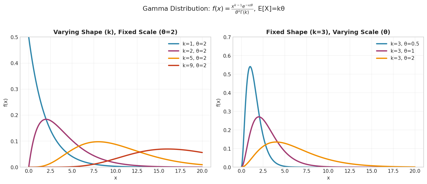
Fig. 15 Gamma distribution parameter effects. Left: Increasing shape \(k\) shifts the mode away from zero and makes the distribution more symmetric. When \(k = 1\), Gamma reduces to Exponential. Right: Increasing scale \(\theta\) stretches the distribution horizontally, increasing both mean and variance.
Historical Context:
The Gamma distribution emerged from studying the gamma function, introduced by Leonhard Euler in 1729. The distribution gained practical importance through Karl Pearson’s work on skewed distributions in the 1890s. It became fundamental in queueing theory through Erlang’s work—the special case with integer shape parameter is called the Erlang distribution. The gamma distribution’s flexibility in modeling positive, skewed data made it invaluable in fields from hydrology to finance.
Properties:
Mean: \(E[X] = \frac{\alpha}{\beta}\)
Variance: \(\text{Var}(X) = \frac{\alpha}{\beta^2}\)
Mode: \(\frac{\alpha-1}{\beta}\) for \(\alpha > 1\)
Moment Generating Function: \(M_X(t) = \left(\frac{\beta}{\beta - t}\right)^\alpha\) for \(t < \beta\)
Special cases:
\(\alpha = 1\): Exponential(β)
\(\alpha = n/2, \beta = 1/2\): Chi-squared with n degrees of freedom
\(\alpha = k\) where \(k \in \mathbb{N}\): Erlang distribution (integer shape parameter)
Theorem: Sum of Exponentials
If \(X_1, ..., X_n\) are independent \(\text{Exp}(\beta)\), then:
Proof (using MGFs):
This is the MGF of \(\text{Gamma}(n, \beta)\).
Theorem: Relationship to Chi-Squared
The chi-squared distribution is a special case of the gamma distribution:
Proof: If \(Z_1, ..., Z_k\) are independent \(\mathcal{N}(0,1)\), then \(\sum Z_i^2 \sim \chi^2(k)\).
Since \(Z^2 \sim \text{Gamma}(1/2, 1/2)\) (can be shown via transformation), the sum follows \(\text{Gamma}(k/2, 1/2)\).
Let’s explore the gamma distribution:
def explore_gamma_distribution():
    """Comprehensive exploration of gamma distribution."""

    fig, ((ax1, ax2), (ax3, ax4)) = plt.subplots(2, 2, figsize=(12, 10))

    # Shape parameter effects
    x = np.linspace(0, 10, 1000)
    beta = 1.0  # Fix rate

    for alpha in [0.5, 1, 2, 5, 10]:
        # Note: SciPy uses scale parameterization, so scale = 1/beta
        pdf = stats.gamma.pdf(x, a=alpha, scale=1/beta)
        label = f'α={alpha}'
        if alpha == 1:
            label += ' (Exponential)'
        ax1.plot(x, pdf, label=label, linewidth=2)

    ax1.set_xlabel('x')
    ax1.set_ylabel('Density')
    ax1.set_title(f'Gamma PDFs with β={beta} (varying shape)')
    ax1.legend()
    ax1.grid(True, alpha=0.3)
    ax1.set_ylim(0, 1.5)

    # Rate parameter effects
    alpha_fixed = 3
    for beta in [0.5, 1, 2, 4]:
        # Note: SciPy uses scale parameterization, so scale = 1/beta
        pdf = stats.gamma.pdf(x, a=alpha_fixed, scale=1/beta)
        ax2.plot(x, pdf, label=f'β={beta}', linewidth=2)

    ax2.set_xlabel('x')
    ax2.set_ylabel('Density')
    ax2.set_title(f'Gamma PDFs with α={alpha_fixed} (varying rate)')
    ax2.legend()
    ax2.grid(True, alpha=0.3)

    # Sum of exponentials
    n_exp = 5
    lam = 2.0
    n_sim = 10000

    # Sum of exponentials
    # Note: NumPy exponential uses scale parameterization
    exp_sum = np.sum([np.random.exponential(1/lam, n_sim)
                     for _ in range(n_exp)], axis=0)

    # Direct gamma - SciPy uses scale = 1/rate
    gamma_samples = stats.gamma.rvs(a=n_exp, scale=1/lam, size=n_sim)

    ax3.hist(exp_sum, bins=50, density=True, alpha=0.5,
             label=f'Sum of {n_exp} Exp({lam})')
    ax3.hist(gamma_samples, bins=50, density=True, alpha=0.5,
             label=f'Gamma({n_exp}, {lam})')

    # Theoretical PDF
    x_theory = np.linspace(0, max(exp_sum.max(), gamma_samples.max()), 1000)
    pdf_theory = stats.gamma.pdf(x_theory, a=n_exp, scale=1/lam)
    ax3.plot(x_theory, pdf_theory, 'r-', linewidth=2, label='Theory')

    ax3.set_xlabel('Value')
    ax3.set_ylabel('Density')
    ax3.set_title('Gamma as Sum of Exponentials')
    ax3.legend()
    ax3.grid(True, alpha=0.3)

    # Chi-squared connection
    x_chi = np.linspace(0, 20, 1000)

    for df in [2, 4, 6]:
        # Chi-squared is Gamma(df/2, 1/2)
        alpha = df / 2
        beta = 0.5

        # Plot both to show they're identical
        chi2_pdf = stats.chi2.pdf(x_chi, df)
        # Note: SciPy gamma uses scale = 1/beta
        gamma_pdf = stats.gamma.pdf(x_chi, a=alpha, scale=1/beta)

        ax4.plot(x_chi, chi2_pdf, '-', linewidth=2, label=f'χ²({df})')
        ax4.plot(x_chi[::20], gamma_pdf[::20], 'o', markersize=5)

    ax4.set_xlabel('x')
    ax4.set_ylabel('Density')
    ax4.set_title('Chi-squared as Gamma: χ²(k) = Gamma(k/2, 1/2)')
    ax4.legend()
    ax4.grid(True, alpha=0.3)
    ax4.set_xlim(0, 20)

    plt.tight_layout()
    plt.show()

explore_gamma_distribution()
Gamma function and factorial relationship:
def explore_gamma_function():
    """Show gamma function properties and relation to factorial."""

    from scipy.special import gamma

    # For integers, Γ(n) = (n-1)!
    print("Gamma function for integers:")
    for n in range(1, 8):
        gamma_val = gamma(n)
        factorial_val = np.math.factorial(n-1) if n > 1 else 1
        print(f"Γ({n}) = {gamma_val:.0f} = {n-1}! = {factorial_val}")

    # Plot gamma function
    x = np.linspace(0.1, 5, 1000)
    y = gamma(x)

    plt.figure(figsize=(10, 6))
    plt.plot(x, y, 'b-', linewidth=2, label='Γ(x)')

    # Mark factorial points
    n_vals = np.arange(1, 6)
    factorial_vals = [gamma(n) for n in n_vals]
    plt.plot(n_vals, factorial_vals, 'ro', markersize=8,
             label='(n-1)! points')

    plt.xlabel('x')
    plt.ylabel('Γ(x)')
    plt.title('The Gamma Function')
    plt.ylim(0, 25)
    plt.legend()
    plt.grid(True, alpha=0.3)
    plt.show()

    # Special values
    print(f"\nSpecial values:")
    print(f"Γ(1/2) = √π = {gamma(0.5):.6f}")
    print(f"Γ(3/2) = √π/2 = {gamma(1.5):.6f}")

explore_gamma_function()
Beta Distribution
Definition
The Beta distribution is a continuous distribution on the interval [0, 1], making it ideal for modeling proportions and probabilities.
Parameterization: Beta(α = shape1, β = shape2)
A random variable \(X \sim \text{Beta}(\alpha, \beta)\) has probability density function:
Historical Context:
The Beta distribution was first studied by Euler and Legendre in connection with the Beta function in the 1730s. It gained statistical prominence through Karl Pearson’s work on the Pearson system of distributions. The Beta distribution’s bounded support makes it natural for modeling proportions, while its flexibility allows it to take many shapes—uniform, U-shaped, bell-shaped, or skewed.
Properties:
Mean: \(E[X] = \frac{\alpha}{\alpha + \beta}\)
Variance: \(\text{Var}(X) = \frac{\alpha\beta}{(\alpha+\beta)^2(\alpha+\beta+1)}\)
Mode: \(\frac{\alpha-1}{\alpha+\beta-2}\) for \(\alpha, \beta > 1\)
Moment Generating Function: No closed form, but moments can be computed
Special cases: - \(\alpha = \beta = 1\): Uniform(0, 1) - \(\alpha = \beta\): Symmetric about 0.5 - \(\alpha = \beta = 0.5\): Arcsine distribution (U-shaped)
Theorem: Order Statistics of Uniform
If \(U_1, ..., U_n\) are independent \(\text{Uniform}(0,1)\) and \(U_{(k)}\) is the \(k\)-th order statistic, then:
Proof: The CDF of \(U_{(k)}\) is:
Taking the derivative:
Relationship: Beta and Gamma
If \(X \sim \text{Gamma}(\alpha, \lambda)\) and \(Y \sim \text{Gamma}(\beta, \lambda)\) are independent, then:
This relationship is fundamental in many applications.
Let’s explore the beta distribution:
def explore_beta_shapes():
    """Explore how α and β affect the Beta distribution shape."""

    x = np.linspace(0, 1, 1000)

    fig, ((ax1, ax2), (ax3, ax4)) = plt.subplots(2, 2, figsize=(12, 10))

    # Different shape combinations
    params_groups = [
        # U-shaped and uniform
        [(0.5, 0.5, 'U-shaped'), (1, 1, 'Uniform')],
        # Symmetric shapes
        [(2, 2, 'Bell'), (5, 5, 'Concentrated'), (10, 10, 'Highly concentrated')],
        # Skewed shapes
        [(2, 5, 'Left skewed'), (5, 2, 'Right skewed')],
        # Extreme shapes
        [(0.5, 2, 'J-shaped'), (2, 0.5, 'Reverse J')]
    ]

    axes = [ax1, ax2, ax3, ax4]
    titles = ['U-shaped and Uniform', 'Symmetric Shapes',
              'Skewed Shapes', 'Extreme Shapes']

    for ax, params, title in zip(axes, params_groups, titles):
        for (a, b, desc) in params:
            pdf = stats.beta.pdf(x, a, b)
            ax.plot(x, pdf, linewidth=2, label=f'α={a}, β={b}: {desc}')

        ax.set_xlabel('x')
        ax.set_ylabel('Density')
        ax.set_title(title)
        ax.legend()
        ax.grid(True, alpha=0.3)
        ax.set_ylim(bottom=0)

    plt.tight_layout()
    plt.show()

explore_beta_shapes()
Order statistics demonstration:
def demonstrate_beta_order_statistics():
    """Show that order statistics of Uniform(0,1) follow Beta."""

    n = 10  # Sample size
    k = 3   # We want the k-th smallest
    n_simulations = 10000

    # Simulate k-th order statistic
    order_stats = []
    for _ in range(n_simulations):
        sample = np.random.uniform(0, 1, n)
        sorted_sample = np.sort(sample)
        order_stats.append(sorted_sample[k-1])  # k-th smallest

    # Theoretical: k-th order statistic ~ Beta(k, n-k+1)
    alpha = k
    beta = n - k + 1

    fig, (ax1, ax2) = plt.subplots(1, 2, figsize=(12, 5))

    # Histogram vs theory
    ax1.hist(order_stats, bins=50, density=True, alpha=0.6,
             label=f'{k}-th order statistic')

    x = np.linspace(0, 1, 1000)
    pdf = stats.beta.pdf(x, alpha, beta)
    ax1.plot(x, pdf, 'r-', linewidth=2,
             label=f'Beta({alpha}, {beta})')

    ax1.set_xlabel('Value')
    ax1.set_ylabel('Density')
    ax1.set_title(f'{k}-th Order Statistic of {n} Uniform(0,1) Variables')
    ax1.legend()
    ax1.grid(True, alpha=0.3)

    # QQ plot
    from scipy.stats import probplot
    probplot(order_stats, dist=stats.beta(alpha, beta), plot=ax2)
    ax2.set_title('Q-Q Plot vs Beta Distribution')
    ax2.grid(True, alpha=0.3)

    plt.tight_layout()
    plt.show()

    # Expected value and quantiles
    print(f"Order statistic: {k}-th out of {n}")
    print(f"Distribution: Beta({alpha}, {beta})")
    print(f"Theoretical mean: {alpha/(alpha+beta):.3f}")
    print(f"Empirical mean: {np.mean(order_stats):.3f}")
    print(f"Theoretical median: {stats.beta.median(alpha, beta):.3f}")
    print(f"Empirical median: {np.median(order_stats):.3f}")

demonstrate_beta_order_statistics()
Beta-Gamma relationship:
def demonstrate_beta_gamma_relationship():
    """Show Beta arises from ratio of Gamma variables."""

    alpha, beta = 3, 5
    lambda_param = 2  # Same rate for both Gammas
    n_sim = 10000

    # Generate independent Gammas
    X = stats.gamma.rvs(a=alpha, scale=1/lambda_param, size=n_sim)
    Y = stats.gamma.rvs(a=beta, scale=1/lambda_param, size=n_sim)

    # Form ratio
    ratio = X / (X + Y)

    # Theoretical Beta
    x = np.linspace(0, 1, 1000)
    beta_pdf = stats.beta.pdf(x, alpha, beta)

    plt.figure(figsize=(10, 6))
    plt.hist(ratio, bins=50, density=True, alpha=0.6,
             label='X/(X+Y) where X~Γ(α,λ), Y~Γ(β,λ)')
    plt.plot(x, beta_pdf, 'r-', linewidth=2,
             label=f'Beta({alpha}, {beta})')

    plt.xlabel('Value')
    plt.ylabel('Density')
    plt.title('Beta Distribution from Gamma Ratio')
    plt.legend()
    plt.grid(True, alpha=0.3)
    plt.show()

    print(f"X ~ Gamma({alpha}, {lambda_param})")
    print(f"Y ~ Gamma({beta}, {lambda_param})")
    print(f"X/(X+Y) ~ Beta({alpha}, {beta})")
    print(f"\nEmpirical mean: {np.mean(ratio):.3f}")
    print(f"Theoretical mean: {alpha/(alpha+beta):.3f}")

demonstrate_beta_gamma_relationship()
Additional Important Distributions
Student’s t-Distribution
Definition
The Student’s t-distribution arises when estimating the mean of a normally distributed population when the sample size is small and population variance is unknown.
Parameterization: t(ν = degrees of freedom)
A random variable \(T \sim t(\nu)\) has probability density function:
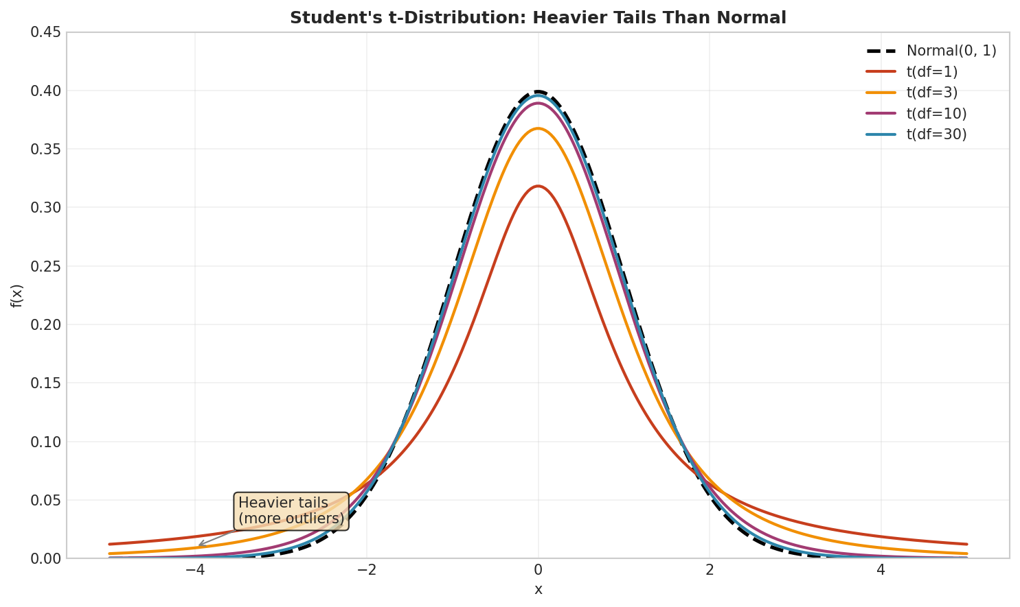
Fig. 16 Student’s t-distribution vs Normal. With low degrees of freedom, the t-distribution has heavier tails than the normal (dashed), accommodating more extreme observations. As \(df \to \infty\), the t-distribution converges to \(N(0, 1)\). The t-distribution with \(df = 1\) is the Cauchy distribution.
Historical Context:
The t-distribution was discovered by William Sealy Gosset around 1905-1906 while working as a chemist at the Guinness brewery in Dublin. Guinness was using statistics to improve beer quality but prohibited employees from publishing trade secrets. Gosset published his findings in Biometrika in 1908 under the pseudonym “Student,” giving us the “Student’s t-distribution.” His specific problem involved small samples—testing beer quality with only 4-5 samples. The normal distribution gave too-narrow confidence intervals for small samples, leading to wrong decisions. The t-distribution corrected this by accounting for the extra uncertainty from estimating variance. This work revolutionized small-sample statistics and remains fundamental to experimental science.
Properties:
Mean: \(E[T] = 0\) for \(\nu > 1\) (undefined for \(\nu = 1\))
Variance: \(\text{Var}(T) = \frac{\nu}{\nu-2}\) for \(\nu > 2\) (undefined for \(1 < \nu \leq 2\))
Heavy tails: Heavier tails than normal distribution
Convergence: As \(\nu \to \infty\), \(t(\nu) \to \mathcal{N}(0,1)\)
Theorem: t-Distribution from Normal and Chi-Square
If \(Z \sim \mathcal{N}(0,1)\) and \(V \sim \chi^2(\nu)\) are independent, then:
Proof: This follows from the ratio of a standard normal to the square root of a scaled chi-square.
In the context of sample means: if \(\bar{X}\) is the sample mean and \(S^2\) is the sample variance from a normal population, then:
Proof: Convergence to Normal
As \(\nu \to \infty\), the t-distribution converges to \(\mathcal{N}(0,1)\):
Using the fact that \(\lim_{n \to \infty} (1 + x/n)^n = e^x\).
Let’s explore the t-distribution:
def explore_t_distribution():
    """Comprehensive exploration of the t-distribution."""

    x = np.linspace(-4, 4, 1000)

    fig, ((ax1, ax2), (ax3, ax4)) = plt.subplots(2, 2, figsize=(12, 10))

    # PDF comparison with normal
    for df in [1, 2, 5, 30]:
        pdf = stats.t.pdf(x, df)
        ax1.plot(x, pdf, label=f't({df})', linewidth=2)

    # Add normal for comparison
    normal_pdf = stats.norm.pdf(x)
    ax1.plot(x, normal_pdf, 'k--', linewidth=2, label='N(0,1)')

    ax1.set_xlabel('x')
    ax1.set_ylabel('Density')
    ax1.set_title("Student's t-Distribution PDFs")
    ax1.legend()
    ax1.grid(True, alpha=0.3)

    # Heavy tails (log scale)
    ax2.semilogy(x[x > 0], stats.t.pdf(x[x > 0], 3),
                 label='t(3)', linewidth=2)
    ax2.semilogy(x[x > 0], stats.norm.pdf(x[x > 0]), 'r--',
                 label='N(0,1)', linewidth=2)

    ax2.set_xlabel('x')
    ax2.set_ylabel('Density (log scale)')
    ax2.set_title('Heavy Tails of t-Distribution')
    ax2.legend()
    ax2.grid(True, alpha=0.3)
    ax2.set_xlim(0, 4)
    ax2.set_ylim(1e-4, 1)

    # Variance as function of df
    df_values = np.arange(3, 31)
    variances = [df/(df-2) for df in df_values]

    ax3.plot(df_values, variances, 'b-', linewidth=2)
    ax3.axhline(y=1, color='red', linestyle='--',
                label='N(0,1) variance = 1')
    ax3.set_xlabel('Degrees of freedom')
    ax3.set_ylabel('Variance')
    ax3.set_title('t-Distribution Variance')
    ax3.legend()
    ax3.grid(True, alpha=0.3)

    # Demonstrate construction from Z and chi-square
    df = 5
    n_sim = 10000

    # Generate t as ratio
    Z = np.random.normal(0, 1, n_sim)
    V = np.random.chisquare(df, n_sim)
    T_constructed = Z / np.sqrt(V / df)

    # Direct t samples
    T_direct = stats.t.rvs(df, size=n_sim)

    ax4.hist(T_constructed, bins=50, density=True, alpha=0.5,
             label='Z/√(V/ν)')
    ax4.hist(T_direct, bins=50, density=True, alpha=0.5,
             label=f'Direct t({df})')

    x_theory = np.linspace(-4, 4, 100)
    ax4.plot(x_theory, stats.t.pdf(x_theory, df), 'r-',
             linewidth=2, label='Theory')

    ax4.set_xlabel('Value')
    ax4.set_ylabel('Density')
    ax4.set_title('t-Distribution as Ratio')
    ax4.legend()
    ax4.grid(True, alpha=0.3)
    ax4.set_xlim(-4, 4)

    plt.tight_layout()
    plt.show()

explore_t_distribution()
Chi-Square Distribution
Definition
The Chi-square distribution with \(k\) degrees of freedom is the distribution of the sum of squares of \(k\) independent standard normal random variables.
Parameterization: χ²(k = degrees of freedom)
If \(Z_1, ..., Z_k\) are independent \(\mathcal{N}(0,1)\), then:
Probability density function:
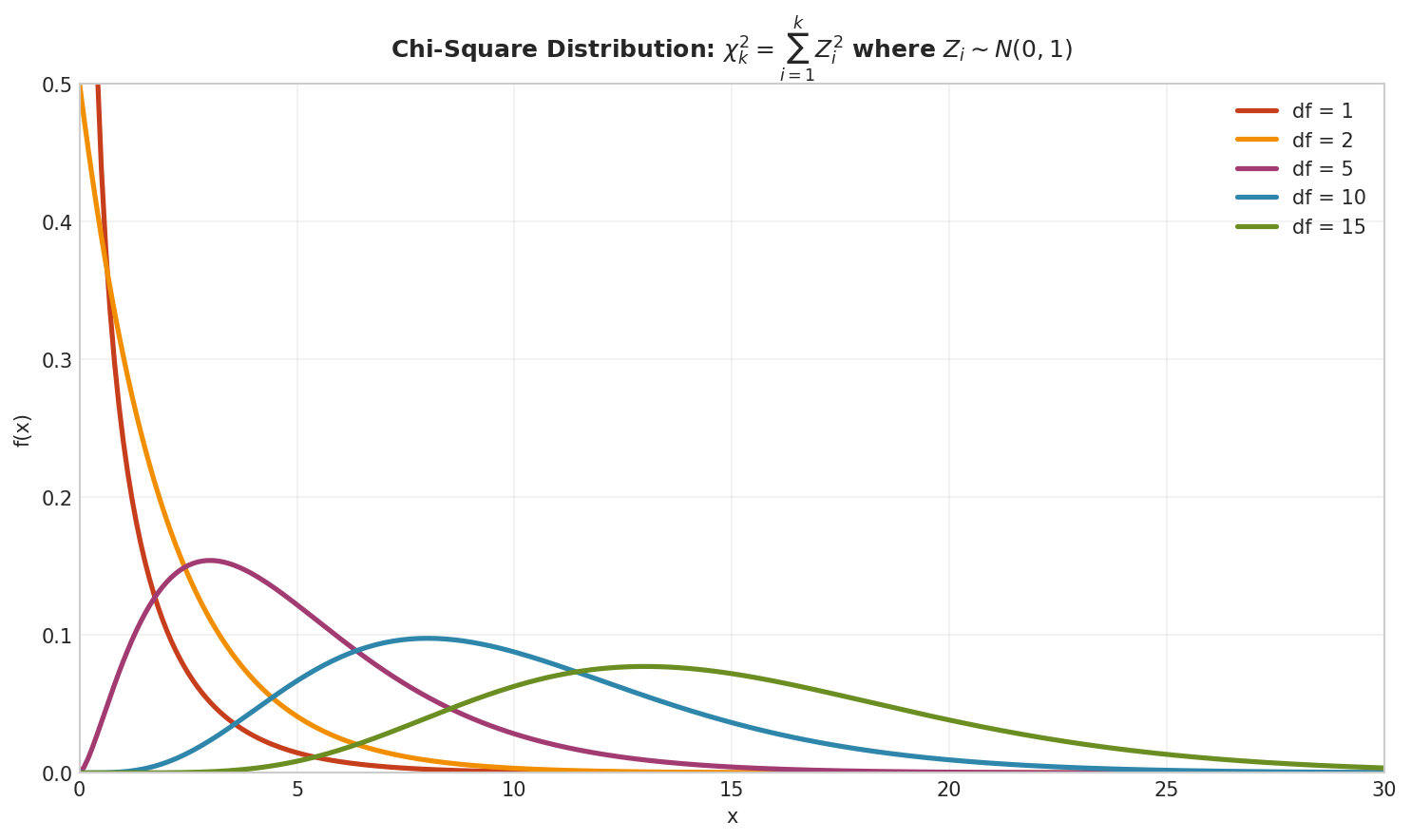
Fig. 17 Chi-square distribution. Defined as the sum of \(k\) squared standard normals, \(\chi^2_k\) is right-skewed for small \(k\) and becomes more symmetric as \(k\) increases. The mean equals \(k\) and variance equals \(2k\). Used extensively in hypothesis testing and variance estimation.
Properties:
Mean: \(E[X] = k\)
Variance: \(\text{Var}(X) = 2k\)
Mode: \(\max(k-2, 0)\)
Moment Generating Function: \(M_X(t) = (1-2t)^{-k/2}\) for \(t < 1/2\)
Relationship to Gamma: \(\chi^2(k) = \text{Gamma}(k/2, 1/2)\)
Additivity: If \(X_i \sim \chi^2(k_i)\) independent, then \(\sum X_i \sim \chi^2(\sum k_i)\)
Theorem: Additivity of Chi-Square
If \(X_1 \sim \chi^2(k_1)\) and \(X_2 \sim \chi^2(k_2)\) are independent, then:
Proof: Using the Gamma representation and MGFs:
Let’s explore the chi-square distribution:
def explore_chi_square():
    """Comprehensive exploration of chi-square distribution."""

    fig, ((ax1, ax2), (ax3, ax4)) = plt.subplots(2, 2, figsize=(12, 10))

    # PDF for different degrees of freedom
    x = np.linspace(0, 20, 1000)

    for df in [1, 2, 3, 5, 10]:
        pdf = stats.chi2.pdf(x, df)
        label = f'k={df}'
        if df == 2:
            label += ' (Exponential(1/2))'
        ax1.plot(x, pdf, label=label, linewidth=2)

    ax1.set_xlabel('x')
    ax1.set_ylabel('Density')
    ax1.set_title('Chi-Square Distribution PDFs')
    ax1.legend()
    ax1.grid(True, alpha=0.3)
    ax1.set_xlim(0, 20)
    ax1.set_ylim(0, 0.5)

    # Connection to squared normals
    df = 5
    n_sim = 10000

    # Sum of squared standard normals
    squared_normals = np.sum(np.random.normal(0, 1, (n_sim, df))**2, axis=1)

    ax2.hist(squared_normals, bins=50, density=True, alpha=0.6,
             label=f'Sum of {df} squared N(0,1)')

    x_theory = np.linspace(0, max(squared_normals), 100)
    pdf_theory = stats.chi2.pdf(x_theory, df)
    ax2.plot(x_theory, pdf_theory, 'r-', linewidth=2,
             label=f'χ²({df})')

    ax2.set_xlabel('Value')
    ax2.set_ylabel('Density')
    ax2.set_title(f'χ² as Sum of Squared Standard Normals')
    ax2.legend()
    ax2.grid(True, alpha=0.3)

    # Additivity property
    k1, k2 = 3, 4
    X1 = stats.chi2.rvs(k1, size=n_sim)
    X2 = stats.chi2.rvs(k2, size=n_sim)
    X_sum = X1 + X2

    ax3.hist(X_sum, bins=50, density=True, alpha=0.6,
             label=f'χ²({k1}) + χ²({k2})')

    x_theory = np.linspace(0, max(X_sum), 100)
    pdf_theory = stats.chi2.pdf(x_theory, k1 + k2)
    ax3.plot(x_theory, pdf_theory, 'r-', linewidth=2,
             label=f'χ²({k1 + k2})')

    ax3.set_xlabel('Value')
    ax3.set_ylabel('Density')
    ax3.set_title('Additivity of Chi-Square')
    ax3.legend()
    ax3.grid(True, alpha=0.3)

    # Mean and variance relationship
    df_values = np.arange(1, 21)

    ax4.scatter(df_values, df_values, label='Mean = k', s=50)
    ax4.scatter(df_values, 2*df_values, label='Variance = 2k', s=50)
    ax4.plot(df_values, df_values, 'b--', alpha=0.5)
    ax4.plot(df_values, 2*df_values, 'r--', alpha=0.5)

    ax4.set_xlabel('Degrees of freedom (k)')
    ax4.set_ylabel('Value')
    ax4.set_title('Chi-Square Mean and Variance')
    ax4.legend()
    ax4.grid(True, alpha=0.3)

    plt.tight_layout()
    plt.show()

explore_chi_square()
F-Distribution
Definition
The F-distribution arises as the ratio of two independent chi-square random variables divided by their respective degrees of freedom.
Parameterization: F(d₁ = numerator df, d₂ = denominator df)
If \(X_1 \sim \chi^2(d_1)\) and \(X_2 \sim \chi^2(d_2)\) are independent, then:
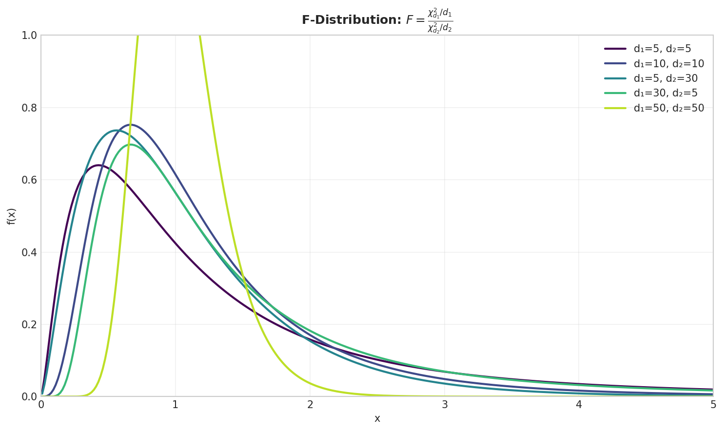
Fig. 18 F-distribution arises as the ratio of two scaled chi-square random variables. It is always right-skewed and positive. Used in ANOVA and regression for comparing variances. The shape depends on both \(d_1\) (numerator df) and \(d_2\) (denominator df).
Historical Context:
The F-distribution is named after Sir Ronald Fisher, though George Snedecor first tabulated it, leading some to call it the Fisher-Snedecor distribution. Fisher developed it in the 1920s for analysis of variance (ANOVA), revolutionizing agricultural research at Rothamsted Experimental Station. The key insight: to test if several groups have equal means, compare variation between groups to variation within groups. If groups truly have equal means, this ratio follows an F-distribution. This enabled testing multiple treatments simultaneously, dramatically improving experimental efficiency.
Properties:
Mean: \(E[F] = \frac{d_2}{d_2-2}\) for \(d_2 > 2\)
Variance: \(\text{Var}(F) = \frac{2d_2^2(d_1+d_2-2)}{d_1(d_2-2)^2(d_2-4)}\) for \(d_2 > 4\)
Mode: \(\frac{d_1-2}{d_1} \cdot \frac{d_2}{d_2+2}\) for \(d_1 > 2\)
Relationship to t: \(t^2(d) = F(1, d)\)
Theorem: Relationship to t-Distribution
If \(T \sim t(d)\), then \(T^2 \sim F(1, d)\)
Proof: From the construction of t-distribution:
Therefore:
Since \(Z^2 \sim \chi^2(1)\), this is the ratio defining \(F(1, d)\).
Let’s explore the F-distribution:
def explore_f_distribution():
    """Comprehensive exploration of F-distribution."""

    fig, ((ax1, ax2), (ax3, ax4)) = plt.subplots(2, 2, figsize=(12, 10))

    # PDF for different parameters
    x = np.linspace(0, 5, 1000)

    params = [(1, 1), (2, 1), (5, 2), (10, 10), (100, 100)]

    for d1, d2 in params:
        pdf = stats.f.pdf(x, d1, d2)
        ax1.plot(x, pdf, label=f'F({d1}, {d2})', linewidth=2)

    ax1.set_xlabel('x')
    ax1.set_ylabel('Density')
    ax1.set_title('F-Distribution PDFs')
    ax1.legend()
    ax1.grid(True, alpha=0.3)
    ax1.set_xlim(0, 5)
    ax1.set_ylim(0, 2)

    # Connection to ratio of chi-squares
    d1, d2 = 5, 10
    n_sim = 10000

    # Generate F as ratio of chi-squares
    chi2_1 = np.random.chisquare(d1, n_sim)
    chi2_2 = np.random.chisquare(d2, n_sim)
    f_ratio = (chi2_1 / d1) / (chi2_2 / d2)

    ax2.hist(f_ratio, bins=50, density=True, alpha=0.6,
             label='(χ²₁/d₁)/(χ²₂/d₂)')

    x_theory = np.linspace(0, 6, 100)
    pdf_theory = stats.f.pdf(x_theory, d1, d2)
    ax2.plot(x_theory, pdf_theory, 'r-', linewidth=2,
             label=f'F({d1}, {d2})')

    ax2.set_xlabel('Value')
    ax2.set_ylabel('Density')
    ax2.set_title('F as Ratio of Scaled Chi-Squares')
    ax2.legend()
    ax2.grid(True, alpha=0.3)
    ax2.set_xlim(0, 6)

    # Relationship to t-distribution
    df = 10
    n_sim = 10000

    # t² equals F(1, df)
    t_samples = stats.t.rvs(df, size=n_sim)
    t_squared = t_samples**2

    f_samples = stats.f.rvs(1, df, size=n_sim)

    ax3.hist(t_squared, bins=50, density=True, alpha=0.5,
             label=f't²({df})')
    ax3.hist(f_samples, bins=50, density=True, alpha=0.5,
             label=f'F(1, {df})')

    x_theory = np.linspace(0, 10, 100)
    pdf_theory = stats.f.pdf(x_theory, 1, df)
    ax3.plot(x_theory, pdf_theory, 'r-', linewidth=2, label='Theory')

    ax3.set_xlabel('Value')
    ax3.set_ylabel('Density')
    ax3.set_title('Relationship: t² = F(1, df)')
    ax3.legend()
    ax3.grid(True, alpha=0.3)
    ax3.set_xlim(0, 10)

    # Effect of degrees of freedom on shape
    x = np.linspace(0, 4, 1000)
    d2_fixed = 10

    for d1 in [1, 2, 5, 10, 20]:
        pdf = stats.f.pdf(x, d1, d2_fixed)
        ax4.plot(x, pdf, label=f'd₁={d1}', linewidth=2)

    ax4.set_xlabel('x')
    ax4.set_ylabel('Density')
    ax4.set_title(f'F-Distribution with d₂={d2_fixed} (varying d₁)')
    ax4.legend()
    ax4.grid(True, alpha=0.3)
    ax4.set_xlim(0, 4)

    plt.tight_layout()
    plt.show()

explore_f_distribution()
Summary and Practical Guidelines
Choosing the Right Distribution
Distribution Selection Guide
For Count Data:
Binomial: Fixed number of trials, constant probability
Poisson: Rare events, no upper limit, mean = variance
Negative Binomial: Overdispersed count data (variance > mean)
Geometric: Time until first success, memoryless property
For Continuous Data:
Normal: Symmetric data, sums of many factors, measurement errors
Exponential: Time between events, constant hazard rate
Gamma: Waiting times, positive skewed data, sum of exponentials
Beta: Proportions, probabilities, bounded data [0,1]
Uniform: Complete uncertainty within bounds, basis for simulation
For Statistical Inference:
t-distribution: Small sample means, unknown variance
Chi-square: Variance estimation, goodness-of-fit tests
F-distribution: Comparing variances, ANOVA, regression significance
Key Relationships Between Distributions
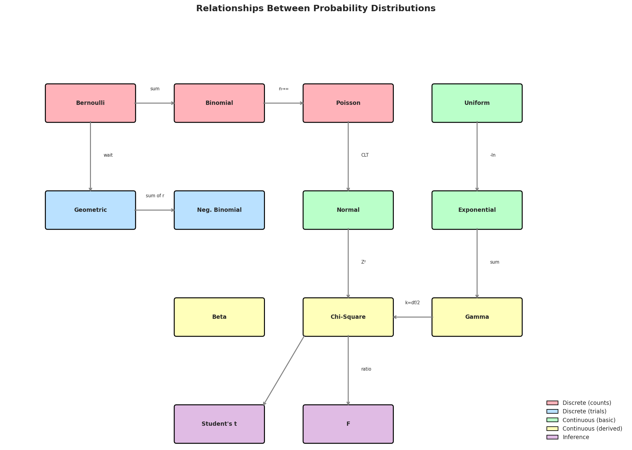
Fig. 19 Relationships between distributions. Arrows indicate how distributions connect: sums of Bernoullis give Binomial; Binomial with \(n \to \infty\) approaches Poisson; Normal arises from the CLT; \(-\ln(U)\) transforms Uniform to Exponential; sums of Exponentials give Gamma; squared Normals give Chi-square; and ratios of Chi-squares give F. Color coding: pink = discrete counts, blue = discrete trials, green = continuous basic, yellow = continuous derived, purple = inference distributions.
Comprehensive Distribution Relationships
1. Limiting Relationships:
\(\text{Binomial}(n, p) \xrightarrow{n \to \infty} \mathcal{N}(np, np(1-p))\) (De Moivre-Laplace)
\(\text{Binomial}(n, p) \xrightarrow{p \to 0, np \to \lambda} \text{Poisson}(\lambda)\) (Poisson limit)
\(t(\nu) \xrightarrow{\nu \to \infty} \mathcal{N}(0, 1)\)
\(\text{Gamma}(\alpha, \beta) \xrightarrow{\alpha \to \infty} \mathcal{N}(\alpha/\beta, \alpha/\beta^2)\) (by CLT)
2. Special Cases:
If \(X \sim \text{Bernoulli}(p)\), then \(X \sim \text{Binomial}(1, p)\)
If \(X \sim \text{Exponential}(\lambda)\), then \(X \sim \text{Gamma}(1, \lambda)\)
If \(X \sim \chi^2(k)\), then \(X \sim \text{Gamma}(k/2, 1/2)\)
If \(X \sim \text{Beta}(1, 1)\), then \(X \sim \text{Uniform}(0, 1)\)
If \(Y \sim \text{Geometric}(p)\) and \(X \sim \text{NegBinomial}(1, p)\), then \(Y = X + 1\) (SciPy convention)
3. Sums and Convolutions:
If \(X_i \sim \text{Bernoulli}(p)\) independent, then \(\sum_{i=1}^n X_i \sim \text{Binomial}(n, p)\)
If \(X_i \sim \text{Exponential}(\lambda)\) independent, then \(\sum_{i=1}^n X_i \sim \text{Gamma}(n, \lambda)\)
If \(Y_i \sim \text{Geometric}(p)\) independent, then \(\sum_{i=1}^n Y_i - n \sim \text{NegBinomial}(n, p)\)
If \(X_i \sim \mathcal{N}(\mu_i, \sigma_i^2)\) independent, then \(\sum_{i=1}^n X_i \sim \mathcal{N}(\sum \mu_i, \sum \sigma_i^2)\)
If \(X_i \sim \chi^2(k_i)\) independent, then \(\sum_{i=1}^n X_i \sim \chi^2(\sum k_i)\)
If \(X_i \sim \text{Gamma}(\alpha_i, \beta)\) independent with same \(\beta\), then \(\sum_{i=1}^n X_i \sim \text{Gamma}(\sum \alpha_i, \beta)\)
4. Transformations:
If \(X \sim \mathcal{N}(0, 1)\), then \(X^2 \sim \chi^2(1)\)
If \(U \sim \text{Uniform}(0, 1)\), then \(-\ln(U)/\lambda \sim \text{Exponential}(\lambda)\)
If \(T \sim t(\nu)\), then \(T^2 \sim F(1, \nu)\)
If \(X \sim \text{Gamma}(\alpha, \lambda)\) and \(Y \sim \text{Gamma}(\beta, \lambda)\), then \(\frac{X}{X+Y} \sim \text{Beta}(\alpha, \beta)\)
5. Constructions:
\(\frac{Z}{\sqrt{V/\nu}} \sim t(\nu)\) where \(Z \sim \mathcal{N}(0,1)\), \(V \sim \chi^2(\nu)\)
\(\frac{U/d_1}{V/d_2} \sim F(d_1, d_2)\) where \(U \sim \chi^2(d_1)\), \(V \sim \chi^2(d_2)\)
\(\min(X_1, ..., X_n) \sim \text{Exponential}(\sum \lambda_i)\) where \(X_i \sim \text{Exponential}(\lambda_i)\)
Python Tools Summary
Essential Python Functions
# Basic operations for any distribution in scipy.stats
from scipy import stats

# For distribution 'dist' with parameters
dist = stats.norm(loc=0, scale=1)  # example with normal

# PDF/PMF
dist.pdf(x)    # Probability density function
dist.pmf(x)    # Probability mass function (discrete)

# CDF and inverse CDF
dist.cdf(x)    # Cumulative distribution function
dist.ppf(q)    # Percent point function (inverse CDF/quantile)

# Random sampling
dist.rvs(size=n, random_state=seed)    # Random variates

# Moments
dist.mean()    # Mean
dist.var()     # Variance
dist.std()     # Standard deviation
dist.moment(n) # n-th moment

# Fitting
params = dist.fit(data)  # Maximum likelihood estimation

# Support
dist.support() # Valid range of values
Parameterization Notes
Important Parameterization Differences
Different libraries and sources use different parameterizations:
Exponential Distribution: - Rate parameterization: \(f(x) = \lambda e^{-\lambda x}\) (used in formulas) - Scale parameterization: \(f(x) = \frac{1}{\theta} e^{-x/\theta}\) where \(\theta = 1/\lambda\) - NumPy uses scale, so use np.random.exponential(scale=1/lambda)
Gamma Distribution: - Shape-Rate: Gamma(α, β) with mean α/β - Shape-Scale: Gamma(α, θ) with mean αθ where θ = 1/β - SciPy uses shape-scale: stats.gamma(a=alpha, scale=1/beta)
Geometric Distribution: - SciPy: Number of trials until first success, support {1, 2, 3, …} - Alternative: Number of failures before first success, support {0, 1, 2, …}
Always check documentation for the specific parameterization used!
Common Pitfalls and Best Practices
Best Practices
Always visualize your data before choosing a distribution
Check assumptions: Many tests assume normality or equal variances
Use appropriate parameterizations: Verify whether using rate or scale
Consider sample size: Small samples need t, not normal
Test goodness-of-fit: Don’t assume, verify with chi-square or K-S tests
Handle edge cases: What happens at boundaries? (e.g., p=0 or p=1)
Use vectorized operations: NumPy is much faster than loops
Set random seeds: For reproducible research
Consider transformations: Log-normal data? Take logs first
Don’t ignore overdispersion: Real count data often has variance > mean
Conclusion
Probability distributions are the fundamental language for describing uncertainty in data science. Through this chapter, we’ve explored:
The computational tools: From Python’s built-in
randommodule to NumPy’s vectorized operations and SciPy’s comprehensive statistical functionsKey distributions: Each with its own story, properties, and applications—from the humble Bernoulli to the sophisticated F-distribution
Mathematical foundations: Rigorous proofs of limit theorems, derivations of properties like memorylessness, and relationships between distributions
Practical implementation: How to generate samples, compute probabilities, and visualize distributions in Python
Historical context: Understanding how these distributions were discovered helps appreciate their significance
Real-world applications: Each distribution solves specific problems in various fields
The ability to work fluently with these distributions—understanding their properties, proving their relationships, and implementing them computationally—forms the foundation for statistical inference, machine learning, and data analysis. As you continue your journey in computational data science, these distributions will appear repeatedly in different contexts, from hypothesis testing to time series analysis to stochastic processes.
Remember: probability distributions are not just mathematical abstractions but practical tools for understanding and quantifying uncertainty in the real world. Master them, and you master a fundamental aspect of data science.
References and Further Reading
Historical Works
Bernoulli, J. (1713). Ars Conjectandi [The Art of Conjecturing]. Thurnisiorum.
de Moivre, A. (1738). The Doctrine of Chances (2nd ed.). Woodfall.
Laplace, P. S. (1812). Théorie analytique des probabilités. Courcier.
Gauss, C. F. (1809). Theoria motus corporum coelestium. Perthes et Besser. Contains the first systematic treatment of the normal distribution in the context of measurement errors.
Poisson, S. D. (1837). Recherches sur la probabilité des jugements en matière criminelle et en matière civile. Bachelier.
Bortkiewicz, L. (1898). Das Gesetz der kleinen Zahlen [The Law of Small Numbers]. Teubner. Classic application of the Poisson distribution to rare events.
Student [Gosset, W. S.] (1908). The probable error of a mean. Biometrika, 6(1), 1–25.
Fisher, R. A. (1925). Statistical Methods for Research Workers. Oliver and Boyd.
Pearson, K. (1895). Contributions to the mathematical theory of evolution. II. Skew variation in homogeneous material. Philosophical Transactions of the Royal Society A, 186, 343–414.
Comprehensive Textbooks
Casella, G., and Berger, R. L. (2002). Statistical Inference (2nd ed.). Duxbury Press.
Ross, S. M. (2019). Introduction to Probability Models (12th ed.). Academic Press.
Johnson, N. L., Kotz, S., and Balakrishnan, N. (1994–1995). Continuous Univariate Distributions (Vols. 1–2, 2nd ed.). Wiley.
Johnson, N. L., Kemp, A. W., and Kotz, S. (2005). Univariate Discrete Distributions (3rd ed.). Wiley.
Wasserman, L. (2004). All of Statistics: A Concise Course in Statistical Inference. Springer.
Computational and Applied
SciPy Community. (2024). SciPy statistical functions documentation. https://docs.scipy.org/doc/scipy/reference/stats.html
NumPy Community. (2024). NumPy random sampling documentation. https://numpy.org/doc/stable/reference/random/index.html