Paradigms of Probability and Statistical Inference

Understanding probability and statistical inference is essential for modern data science. Whether we are simulating complex stochastic systems, quantifying prediction confidence, or choosing between competing models, we must first confront a fundamental question: What does probability mean? The answer shapes not only our philosophical perspective but also our computational methods, our interpretation of results, and ultimately the questions we can answer with data.

This chapter establishes the mathematical and philosophical foundation for all computational methods in this course. We will see that while everyone agrees on the mathematical rules governing probability (Kolmogorov’s axioms), profound disagreements exist about what these numbers actually represent—and these disagreements lead to radically different approaches to statistical inference.

Road Map 🧭

• Understand: Kolmogorov’s axiomatic foundation and why it’s interpretation-neutral

• Develop: Ability to distinguish frequentist, Bayesian, and likelihood-based reasoning

• Implement: Basic probability calculations in Python that work across all paradigms

• Evaluate: When to apply different inference frameworks based on problem structure and goals

The Mathematical Foundation: Kolmogorov’s Axioms

Before discussing what probability means philosophically, we must establish its mathematical foundation. In 1933, Andrey Kolmogorov provided a rigorous axiomatic framework that unified centuries of probabilistic thinking and that all modern approaches accept, regardless of their philosophical interpretation.

The Probability Space

All of probability theory is built on the concept of a probability space. In full mathematical generality, this is formalized using measure theory as a triple \((\Omega, \mathcal{F}, P)\) involving σ-algebras. However, for computational data science, we can work with a more intuitive framework that covers all practical cases.

Note on Mathematical Rigor 📚

In advanced probability theory, σ-algebras (collections of “measurable” events) are essential for handling continuous probability spaces rigorously. Throughout this course, we’ll work with the simplified framework below, which is sufficient for all computational applications. Readers interested in measure-theoretic foundations can consult Billingsley (1995) or Durrett (2019).

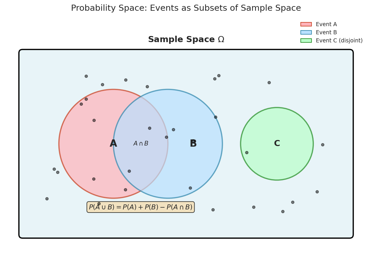
Fig. 1 A probability space consists of a sample space Ω (rectangle) containing all possible outcomes, with events as subsets. Events A and B overlap, illustrating \(P(A \cup B) = P(A) + P(B) - P(A \cap B)\). Event C is disjoint from both.

For this course, a probability space consists of:

• \(\Omega\) is the sample space—the set of all possible outcomes of a random experiment.

  • For a coin flip: \(\Omega = \{H, T\}\)

  • For a die roll: \(\Omega = \{1, 2, 3, 4, 5, 6\}\)

  • For measuring a continuous quantity: \(\Omega = \mathbb{R}\) or an interval like \([0, 1]\)

• Events are subsets of \(\Omega\) to which we can assign probabilities.

  • In discrete spaces: any subset is an event

  • In continuous spaces: “reasonable” subsets (intervals, unions of intervals, etc.) are events

• \(P\) is a probability measure—a function assigning probabilities to events that satisfies Kolmogorov’s axioms.

Kolmogorov’s Three Axioms

For computational work, we can state Kolmogorov’s axioms in an accessible form that works for both discrete and continuous probability spaces:

Axiom 1 (Non-negativity): For any event \(E\),

\[P(E) \geq 0\]

Probabilities cannot be negative—they represent a degree of certainty that is at minimum zero.

Axiom 2 (Normalization): The probability of the entire sample space is unity,

\[P(\Omega) = 1\]

Something in the sample space must occur with certainty.

Axiom 3 (Additivity): For any countable sequence of pairwise disjoint events \(E_1, E_2, E_3, \ldots\) where \(E_i \cap E_j = \emptyset\) for \(i \neq j\),

\[P\left(\bigcup_{i=1}^{\infty} E_i\right) = \sum_{i=1}^{\infty} P(E_i)\]

If events cannot occur simultaneously (are mutually exclusive), the probability that at least one occurs equals the sum of their individual probabilities.

In practice: For finite sample spaces (dice, coins, cards), we only need finite additivity. For continuous spaces (normal distribution, exponential distribution), the full countable additivity ensures consistency when dealing with limits and infinite sums.

From these three axioms, we can derive all familiar properties of probability:

• \(P(\emptyset) = 0\) (the impossible event has probability zero)

• \(0 \leq P(E) \leq 1\) for any event \(E\)

• \(P(E^c) = 1 - P(E)\) (complement rule)

• \(P(A \cup B) = P(A) + P(B) - P(A \cap B)\) (inclusion-exclusion)

• If \(A \subseteq B\), then \(P(A) \leq P(B)\) (monotonicity)

Computational Perspective

In Python, we represent probability spaces through data structures and functions. For discrete sample spaces, we can use dictionaries; for continuous spaces, we rely on probability density functions from libraries like SciPy.

Algorithm: Discrete Probability Space Construction

Input: Sample space Ω = {ω₁, ω₂, ..., ωₙ}, probability function p: Ω → [0,1]
Output: Valid probability space or error

1. Verify non-negativity: Check p(ωᵢ) ≥ 0 for all i
2. Verify normalization: Check Σᵢ p(ωᵢ) = 1 (within numerical tolerance)
3. If valid, return probability space representation
4. Else, raise ValueError with specific axiom violation

Computational Complexity: O(n) for verification of a discrete probability space with n outcomes.

Python Implementation

import numpy as np
from typing import Dict, Union

class DiscreteProbabilitySpace:
    """
    Represents a discrete probability space satisfying Kolmogorov's axioms.

    Parameters
    ----------
    outcomes : list
        Sample space Ω - list of possible outcomes
    probabilities : list or dict
        Probability mass function - either list of probabilities
        (same order as outcomes) or dict mapping outcomes to probabilities
    tol : float, optional
        Numerical tolerance for normalization check (default 1e-10)
    """

    def __init__(self, outcomes, probabilities, tol=1e-10):
        self.outcomes = outcomes

        # Convert to dictionary for convenient lookup
        if isinstance(probabilities, dict):
            self.pmf = probabilities
        else:
            self.pmf = dict(zip(outcomes, probabilities))

        # Verify Kolmogorov's axioms
        self._verify_axioms(tol)

    def _verify_axioms(self, tol):
        """Verify non-negativity and normalization."""
        # Axiom 1: Non-negativity
        for outcome, prob in self.pmf.items():
            if prob < 0:
                raise ValueError(f"Axiom 1 violated: P({outcome}) = {prob} < 0")

        # Axiom 2: Normalization
        total_prob = sum(self.pmf.values())
        if abs(total_prob - 1.0) > tol:
            raise ValueError(
                f"Axiom 2 violated: Total probability = {total_prob} ≠ 1"
            )

        # Axiom 3: For discrete finite spaces, additivity is satisfied by
        # construction when we compute event probabilities as sums over
        # disjoint outcomes.

    def prob(self, event):
        """
        Calculate probability of an event.

        Parameters
        ----------
        event : callable or iterable
            Either a function returning True for outcomes in event,
            or an iterable of outcomes in the event

        Returns
        -------
        float
            Probability of the event
        """
        if callable(event):
            # Event defined by indicator function
            return sum(self.pmf[outcome] for outcome in self.outcomes
                      if event(outcome))
        else:
            # Event defined as set of outcomes
            return sum(self.pmf.get(outcome, 0) for outcome in event)

    def complement_prob(self, event):
        """Calculate P(E^c) = 1 - P(E)."""
        return 1.0 - self.prob(event)

Example 💡: Fair Die Probability Space

Given: A fair six-sided die with outcomes {1, 2, 3, 4, 5, 6}.

Find: Verify Kolmogorov’s axioms and compute probabilities of compound events.

Mathematical approach:

The sample space is \(\Omega = \{1, 2, 3, 4, 5, 6\}\). For a fair die, each outcome has equal probability:

\[P(\{\omega\}) = \frac{1}{6} \quad \text{for each } \omega \in \Omega\]

Verify Axiom 1 (Non-negativity): \(P(\{\omega\}) = 1/6 > 0\) ✓

Verify Axiom 2 (Normalization):

\[P(\Omega) = \sum_{i=1}^{6} P(\{i\}) = 6 \times \frac{1}{6} = 1 \quad ✓\]

Verify Axiom 3 (Countable Additivity): For disjoint events \(E_1 = \{2, 4, 6\}\) (even) and \(E_2 = \{1, 3, 5\}\) (odd):

\[P(E_1 \cup E_2) = P(\Omega) = 1 = \frac{3}{6} + \frac{3}{6} = P(E_1) + P(E_2) \quad ✓\]

Python implementation:

# Create fair die probability space
die = DiscreteProbabilitySpace(
    outcomes=[1, 2, 3, 4, 5, 6],
    probabilities=[1/6, 1/6, 1/6, 1/6, 1/6, 1/6]
)

# Compute probability of rolling even
even_prob = die.prob([2, 4, 6])
print(f"P(even) = {even_prob:.4f}")  # 0.5000

# Compute probability of rolling greater than 4
greater_than_4 = die.prob(lambda x: x > 4)
print(f"P(X > 4) = {greater_than_4:.4f}")  # 0.3333

# Verify complement rule: P(even) + P(odd) = 1
odd_prob = die.complement_prob([2, 4, 6])
print(f"P(odd) = {odd_prob:.4f}")  # 0.5000
print(f"P(even) + P(odd) = {even_prob + odd_prob:.4f}")  # 1.0000

Result: All axioms verified. P(even) = 0.5, P(X > 4) = 0.3333, complement rule holds numerically.

Why This Matters 💡

These axioms are interpretation-neutral—they specify how probabilities must behave mathematically without dictating what probability actually means. All major schools of statistical thought (frequentist, Bayesian, likelihoodist) accept these axioms, yet they fundamentally disagree about how to interpret probability values and conduct inference. The axioms provide a common mathematical language while leaving philosophical room for different interpretations.

Why This Matters 💡

These axioms are interpretation-neutral—they specify how probabilities must behave mathematically without dictating what probability actually means. All major schools of statistical thought (frequentist, Bayesian, likelihoodist) accept these axioms, yet they fundamentally disagree about how to interpret probability values and conduct inference. The axioms provide a common mathematical language while leaving philosophical room for different interpretations.

Mathematical Preliminaries: Random Variables: Connecting Events to Numbers

While Kolmogorov’s axioms assign probabilities to events (subsets of the sample space), data science typically deals with numerical outcomes. A random variable provides this connection:

Definition: Random Variable

A random variable \(X\) is a function from the sample space to the real numbers:

\[X: \Omega \to \mathbb{R}\]

For this course, we work with random variables without formal measure-theoretic details. Intuitively, \(X\) assigns a numerical value to each outcome \(\omega \in \Omega\).

Example: Consider flipping a coin twice.

• Sample space: \(\Omega = \{HH, HT, TH, TT\}\)

• Random variable \(X\) = “number of heads”

• Mapping: \(X(HH) = 2, X(HT) = 1, X(TH) = 1, X(TT) = 0\)

The random variable \(X\) transforms events about outcomes (“got HT”) into events about numbers (\(X = 1\)). This allows us to write:

\[P(X = 1) = P(\{HT, TH\}) = P(HT) + P(TH) = \frac{1}{4} + \frac{1}{4} = \frac{1}{2}\]

Types of Random Variables:

• Discrete: Takes countable values (e.g., \(\{0, 1, 2, \ldots\}\) or \(\{0, 1\}\))

• Continuous: Takes uncountable values in an interval (e.g., \([0, 1]\) or \(\mathbb{R}\))

The type determines which mathematical tools we use to describe the distribution.

Probability Mass Functions (PMF): Discrete Distributions

For discrete random variables, the probability mass function directly specifies the probability of each value.

Definition: Probability Mass Function (PMF)

For a discrete random variable \(X\), the probability mass function is:

\[p_X(x) = P(X = x)\]

The PMF must satisfy:

1. Non-negativity: \(p_X(x) \geq 0\) for all \(x\)

2. Normalization: \(\sum_{\text{all } x} p_X(x) = 1\)

Key properties:

• The PMF gives exact probabilities for discrete values

• \(P(X \in A) = \sum_{x \in A} p_X(x)\) for any set \(A\)

• The PMF inherits non-negativity and normalization from Kolmogorov’s axioms

Example 💡: Fair Die PMF

Given: Roll a fair six-sided die. Let \(X\) = outcome.

Find: The PMF and verify it satisfies the axioms.

Solution:

The sample space is \(\Omega = \{1, 2, 3, 4, 5, 6\}\), and each outcome has probability \(1/6\) (fair die). The PMF is:

\[\begin{split}p_X(x) = \begin{cases} \frac{1}{6} & \text{if } x \in \{1, 2, 3, 4, 5, 6\} \\ 0 & \text{otherwise} \end{cases}\end{split}\]

Verify non-negativity: \(p_X(x) = 1/6 > 0\) for all valid \(x\) ✓

Verify normalization:

\[\sum_{x=1}^{6} p_X(x) = 6 \times \frac{1}{6} = 1 \quad ✓\]

Compute probabilities:

\[P(X \text{ is even}) = P(X \in \{2, 4, 6\}) = p_X(2) + p_X(4) + p_X(6) = \frac{3}{6} = \frac{1}{2}\]

\[P(X > 4) = p_X(5) + p_X(6) = \frac{2}{6} = \frac{1}{3}\]

Python implementation:

import numpy as np
import matplotlib.pyplot as plt

# Define the PMF
outcomes = np.array([1, 2, 3, 4, 5, 6])
pmf = np.array([1/6, 1/6, 1/6, 1/6, 1/6, 1/6])

# Verify normalization
print(f"Sum of PMF: {np.sum(pmf)}")  # Should be 1.0

# Compute probabilities
prob_even = np.sum(pmf[[1, 3, 5]])  # indices for 2, 4, 6
print(f"P(X is even): {prob_even}")

# Visualize PMF
plt.figure(figsize=(8, 5))
plt.stem(outcomes, pmf, basefmt=" ")
plt.xlabel('Outcome (x)')
plt.ylabel('P(X = x)')
plt.title('PMF of Fair Die')
plt.ylim(0, 0.25)
plt.grid(True, alpha=0.3)
plt.show()

Result: The PMF clearly shows equal probability mass on each outcome, characteristic of a uniform discrete distribution.

Probability Density Functions (PDF): Continuous Distributions

For continuous random variables, the probability of any exact value is zero: \(P(X = x) = 0\). Instead, we work with probabilities of intervals using the probability density function.

Definition: Probability Density Function (PDF)

For a continuous random variable \(X\), the probability density function \(f_X(x)\) satisfies:

\[P(a \leq X \leq b) = \int_a^b f_X(x) \, dx\]

The PDF must satisfy:

1. Non-negativity: \(f_X(x) \geq 0\) for all \(x\)

2. Normalization: \(\int_{-\infty}^{\infty} f_X(x) \, dx = 1\)

Critical distinctions from PMF:

• \(f_X(x)\) is not a probability—it’s a density

• \(f_X(x)\) can be greater than 1 (unlike PMF)

• \(P(X = x) = 0\) for any specific \(x\)

• Only intervals have non-zero probability

Intuition: The PDF describes how probability is “spread” over the real line. Think of it as probability per unit length:

\[P(x < X \leq x + dx) \approx f_X(x) \cdot dx \quad \text{for small } dx\]

Example 💡: Uniform(0, 1) PDF

Given: A random variable \(X\) uniformly distributed on \([0, 1]\).

Find: The PDF, verify properties, and compute probabilities.

Solution:

For uniform distribution on \([0, 1]\), the PDF is:

\[\begin{split}f_X(x) = \begin{cases} 1 & \text{if } 0 \leq x \leq 1 \\ 0 & \text{otherwise} \end{cases}\end{split}\]

Verify non-negativity: \(f_X(x) = 1 \geq 0\) on support ✓

Verify normalization:

\[\int_{-\infty}^{\infty} f_X(x) \, dx = \int_0^1 1 \, dx = 1 \quad ✓\]

Note: \(f_X(0.5) = 1\), which is not a probability. It means probability density is 1 unit per unit length.

Compute probabilities:

\[P(0.2 \leq X \leq 0.7) = \int_{0.2}^{0.7} 1 \, dx = 0.7 - 0.2 = 0.5\]

\[P(X = 0.5) = \int_{0.5}^{0.5} 1 \, dx = 0 \quad \text{(exact point has zero probability)}\]

\[P(X \leq 0.3) = \int_0^{0.3} 1 \, dx = 0.3\]

Python implementation:

import numpy as np
import matplotlib.pyplot as plt

# Define PDF
def uniform_pdf(x):
    return np.where((x >= 0) & (x <= 1), 1.0, 0.0)

# Visualize PDF
x = np.linspace(-0.5, 1.5, 1000)
pdf_values = uniform_pdf(x)

plt.figure(figsize=(10, 6))
plt.plot(x, pdf_values, 'b-', linewidth=2, label='PDF')
plt.fill_between(x, 0, pdf_values, alpha=0.3)

# Highlight P(0.2 ≤ X ≤ 0.7)
x_interval = x[(x >= 0.2) & (x <= 0.7)]
plt.fill_between(x_interval, 0, uniform_pdf(x_interval),
                 alpha=0.5, color='red', label='P(0.2 ≤ X ≤ 0.7) = 0.5')

plt.xlabel('x')
plt.ylabel('f(x)')
plt.title('PDF of Uniform(0, 1)')
plt.legend()
plt.grid(True, alpha=0.3)
plt.ylim(0, 1.5)
plt.show()

# Verify normalization numerically
from scipy import integrate
integral, _ = integrate.quad(uniform_pdf, -np.inf, np.inf)
print(f"Integral of PDF: {integral:.10f}")  # Should be 1.0

# Compute probability using scipy
from scipy import stats
uniform_dist = stats.uniform(loc=0, scale=1)
prob = uniform_dist.cdf(0.7) - uniform_dist.cdf(0.2)
print(f"P(0.2 ≤ X ≤ 0.7): {prob}")

Result: The PDF is flat at height 1 over \([0, 1]\), representing equal density everywhere. The shaded area equals the probability.

Common Misconception ⚠️

Wrong: “If \(f_X(5) = 2.3\), then \(P(X = 5) = 2.3\)”

Right: “\(f_X(5) = 2.3\) means the probability density at \(x = 5\) is 2.3. The actual probability \(P(X = 5) = 0\) for any continuous distribution. We can only compute \(P(a \leq X \leq b)\) for intervals.”

Physical analogy: Think of PDF like mass density. A steel beam might have density 7850 kg/m³ at a point, but the mass of an exact point is zero. Only intervals have mass, just as only intervals have probability.

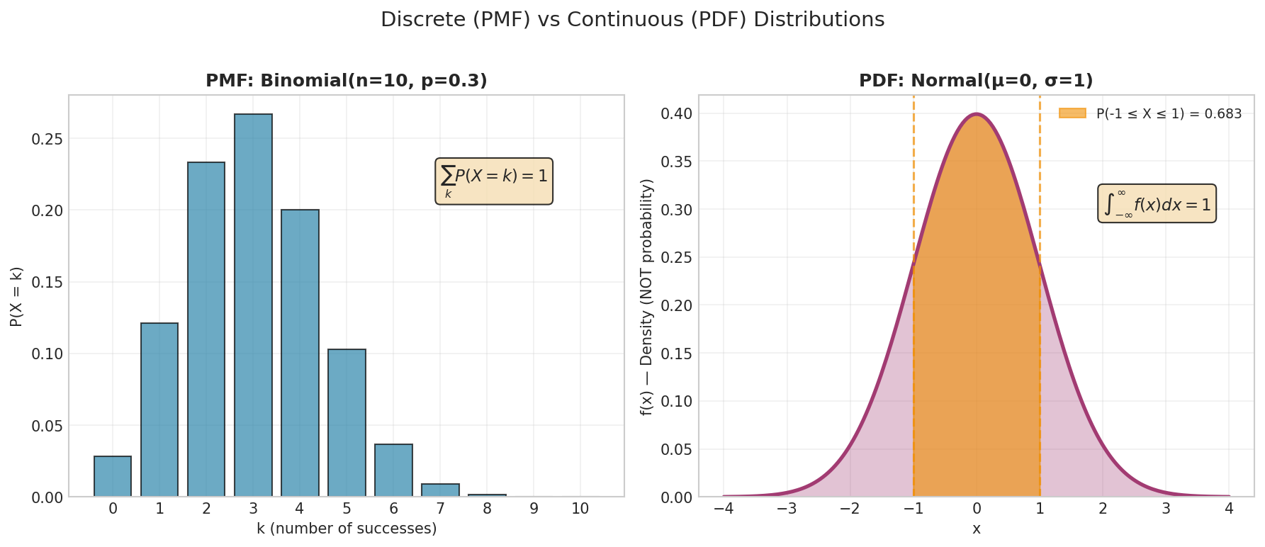
Fig. 2 Left: Probability Mass Function (PMF) for Binomial(10, 0.3)—each bar represents the exact probability \(P(X = k)\). Right: Probability Density Function (PDF) for Normal(0, 1)—the shaded area represents \(P(-1 \leq X \leq 1) \approx 0.683\). Note that PDF values are densities, not probabilities.

Cumulative Distribution Functions (CDF): Universal Description

The cumulative distribution function works for both discrete and continuous random variables, providing a unified framework.

Definition: Cumulative Distribution Function (CDF)

For any random variable \(X\), the cumulative distribution function is:

\[F_X(x) = P(X \leq x)\]

The CDF must satisfy:

1. Monotonicity: If \(x_1 \leq x_2\), then \(F_X(x_1) \leq F_X(x_2)\)

2. Right-continuous: \(\lim_{h \to 0^+} F_X(x + h) = F_X(x)\)

3. Limits: \(\lim_{x \to -\infty} F_X(x) = 0\) and \(\lim_{x \to \infty} F_X(x) = 1\)

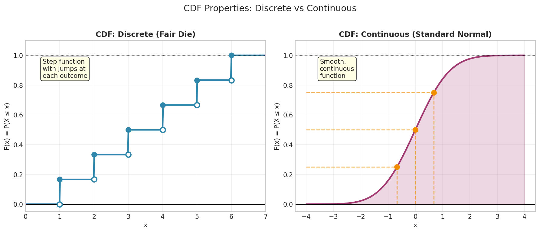
Fig. 3 Left: CDF for a discrete distribution (fair die) is a step function with jumps at each outcome. Open circles indicate left-limits; closed circles indicate the CDF value. Right: CDF for a continuous distribution (standard normal) is smooth and strictly increasing, with quartiles marked.

Relationships to PMF and PDF:

For discrete \(X\):

\[F_X(x) = \sum_{x_i \leq x} p_X(x_i)\]

For continuous \(X\):

\[F_X(x) = \int_{-\infty}^{x} f_X(t) \, dt\]

And conversely (for continuous):

\[f_X(x) = \frac{d}{dx} F_X(x)\]

Computing probabilities from CDF:

\[P(a < X \leq b) = F_X(b) - F_X(a)\]

\[P(X > a) = 1 - F_X(a)\]

\[P(X = a) = F_X(a) - \lim_{h \to 0^+} F_X(a - h) \quad \text{(discrete only)}\]

Example 💡: CDF for Fair Die

Given: Fair die with \(X \in \{1, 2, 3, 4, 5, 6\}\), each with probability \(1/6\).

Find: The CDF and use it to compute probabilities.

Solution:

Build the CDF by accumulating probabilities:

\[\begin{split}F_X(x) = P(X \leq x) = \begin{cases} 0 & \text{if } x < 1 \\ 1/6 & \text{if } 1 \leq x < 2 \\ 2/6 & \text{if } 2 \leq x < 3 \\ 3/6 & \text{if } 3 \leq x < 4 \\ 4/6 & \text{if } 4 \leq x < 5 \\ 5/6 & \text{if } 5 \leq x < 6 \\ 1 & \text{if } x \geq 6 \end{cases}\end{split}\]

The CDF is a step function for discrete random variables, with jumps at each possible value.

Compute probabilities:

\[P(X \leq 4) = F_X(4) = \frac{4}{6} = \frac{2}{3}\]

\[P(2 < X \leq 5) = F_X(5) - F_X(2) = \frac{5}{6} - \frac{2}{6} = \frac{1}{2}\]

\[P(X = 3) = F_X(3) - F_X(3^-) = \frac{3}{6} - \frac{2}{6} = \frac{1}{6}\]

Python implementation:

import numpy as np
import matplotlib.pyplot as plt
from scipy import stats

# Define the die distribution
outcomes = np.arange(1, 7)
pmf = np.ones(6) / 6

# Compute CDF manually
def compute_cdf(x):
    return np.sum(pmf[outcomes <= x])

# Vectorize for plotting
compute_cdf_vec = np.vectorize(compute_cdf)

# Plot PMF and CDF
fig, (ax1, ax2) = plt.subplots(1, 2, figsize=(12, 5))

# PMF (stick plot)
ax1.stem(outcomes, pmf, basefmt=" ")
ax1.set_xlabel('x')
ax1.set_ylabel('P(X = x)')
ax1.set_title('PMF of Fair Die')
ax1.grid(True, alpha=0.3)
ax1.set_ylim(0, 0.25)

# CDF (step function)
x_plot = np.linspace(0, 7, 1000)
cdf_plot = compute_cdf_vec(x_plot)
ax2.plot(x_plot, cdf_plot, 'b-', linewidth=2)
ax2.scatter(outcomes, np.cumsum(pmf), color='red', s=50, zorder=5)
ax2.set_xlabel('x')
ax2.set_ylabel('F(x) = P(X ≤ x)')
ax2.set_title('CDF of Fair Die')
ax2.grid(True, alpha=0.3)
ax2.set_ylim(-0.1, 1.1)

plt.tight_layout()
plt.show()

# Using SciPy
die_dist = stats.randint(1, 7)  # discrete uniform on {1,2,3,4,5,6}
print(f"P(X ≤ 4): {die_dist.cdf(4)}")
print(f"P(2 < X ≤ 5): {die_dist.cdf(5) - die_dist.cdf(2)}")

Result: The CDF shows characteristic “staircase” pattern for discrete distributions, jumping at each possible value.

Example 💡: CDF for Uniform(0, 1)

Given: \(X \sim \text{Uniform}(0, 1)\) with PDF \(f_X(x) = 1\) on \([0, 1]\).

Find: Derive the CDF.

Solution:

For \(x < 0\): No probability mass to the left, so \(F_X(x) = 0\).

For \(0 \leq x \leq 1\):

\[F_X(x) = \int_{-\infty}^{x} f_X(t) \, dt = \int_0^x 1 \, dt = x\]

For \(x > 1\): All probability mass is to the left, so \(F_X(x) = 1\).

Therefore:

\[\begin{split}F_X(x) = \begin{cases} 0 & \text{if } x < 0 \\ x & \text{if } 0 \leq x \leq 1 \\ 1 & \text{if } x > 1 \end{cases}\end{split}\]

The CDF is a continuous function for continuous random variables (no jumps).

Verify by differentiation:

\[f_X(x) = \frac{d}{dx} F_X(x) = \frac{d}{dx}(x) = 1 \quad \text{for } 0 \leq x \leq 1 \quad ✓\]

Python implementation:

import numpy as np
import matplotlib.pyplot as plt
from scipy import stats

# Define PDF and CDF
def uniform_pdf(x):
    return np.where((x >= 0) & (x <= 1), 1.0, 0.0)

def uniform_cdf(x):
    return np.where(x < 0, 0.0, np.where(x > 1, 1.0, x))

# Plot
x = np.linspace(-0.5, 1.5, 1000)

fig, (ax1, ax2) = plt.subplots(1, 2, figsize=(12, 5))

# PDF
ax1.plot(x, uniform_pdf(x), 'b-', linewidth=2)
ax1.fill_between(x, 0, uniform_pdf(x), alpha=0.3)
ax1.set_xlabel('x')
ax1.set_ylabel('f(x)')
ax1.set_title('PDF of Uniform(0, 1)')
ax1.grid(True, alpha=0.3)
ax1.set_ylim(0, 1.5)

# CDF
ax2.plot(x, uniform_cdf(x), 'b-', linewidth=2)
ax2.set_xlabel('x')
ax2.set_ylabel('F(x) = P(X ≤ x)')
ax2.set_title('CDF of Uniform(0, 1)')
ax2.grid(True, alpha=0.3)
ax2.set_ylim(-0.1, 1.1)

# Add specific probability
a, b = 0.2, 0.7
ax2.axvline(a, color='red', linestyle='--', alpha=0.5)
ax2.axvline(b, color='red', linestyle='--', alpha=0.5)
ax2.plot([a, b], [uniform_cdf(a), uniform_cdf(b)], 'ro', markersize=8)
ax2.annotate(f'P({a} < X ≤ {b}) = {b - a}',
             xy=(0.45, 0.45), fontsize=12, color='red')

plt.tight_layout()
plt.show()

# Using SciPy
uniform_dist = stats.uniform(0, 1)
print(f"F(0.5): {uniform_dist.cdf(0.5)}")
print(f"P(0.2 < X ≤ 0.7): {uniform_dist.cdf(0.7) - uniform_dist.cdf(0.2)}")

Result: The CDF is a straight line from (0, 0) to (1, 1), showing linear accumulation of probability.

Quantile Function (Inverse CDF)

The quantile function (or inverse CDF) is crucial for random number generation and statistical inference.

Definition: Quantile Function

For a random variable \(X\) with CDF \(F_X\), the quantile function (or percent point function) is:

\[F_X^{-1}(p) = \inf\{x : F_X(x) \geq p\} \quad \text{for } 0 < p < 1\]

This gives the value \(x\) such that \(P(X \leq x) = p\).

Common quantiles:

• \(F_X^{-1}(0.5)\) = median

• \(F_X^{-1}(0.25)\), \(F_X^{-1}(0.75)\) = quartiles

• \(F_X^{-1}(0.025)\), \(F_X^{-1}(0.975)\) = boundaries of central 95%

Key property (Probability Integral Transform): If \(U \sim \text{Uniform}(0, 1)\), then:

\[X = F_X^{-1}(U) \text{ has CDF } F_X\]

This is the foundation for the inverse transform method of random number generation (Chapter 2).

Example 💡: Quantiles for Exponential Distribution

Given: \(X \sim \text{Exponential}(\lambda)\) with CDF \(F_X(x) = 1 - e^{-\lambda x}\) for \(x \geq 0\).

Find: The quantile function and specific quantiles.

Solution:

To find \(F_X^{-1}(p)\), solve \(F_X(x) = p\):

\[1 - e^{-\lambda x} = p\]

\[e^{-\lambda x} = 1 - p\]

\[-\lambda x = \ln(1 - p)\]

\[x = -\frac{\ln(1 - p)}{\lambda}\]

Therefore, the quantile function is:

\[F_X^{-1}(p) = -\frac{\ln(1 - p)}{\lambda}\]

Compute specific quantiles for \(\lambda = 1\):

• Median: \(F_X^{-1}(0.5) = -\ln(0.5) = \ln(2) \approx 0.693\)

• First quartile: \(F_X^{-1}(0.25) = -\ln(0.75) \approx 0.288\)

• 95th percentile: \(F_X^{-1}(0.95) = -\ln(0.05) \approx 2.996\)

Python implementation:

import numpy as np
import matplotlib.pyplot as plt
from scipy import stats

lam = 1.0  # rate parameter
exp_dist = stats.expon(scale=1/lam)

# Plot CDF and quantile function
fig, (ax1, ax2) = plt.subplots(1, 2, figsize=(12, 5))

# CDF
x = np.linspace(0, 5, 1000)
cdf = exp_dist.cdf(x)
ax1.plot(x, cdf, 'b-', linewidth=2, label='F(x)')

# Mark quantiles
quantiles_p = [0.25, 0.5, 0.75, 0.95]
quantiles_x = [exp_dist.ppf(p) for p in quantiles_p]

for p, q in zip(quantiles_p, quantiles_x):
    ax1.plot([q, q], [0, p], 'r--', alpha=0.5)
    ax1.plot([0, q], [p, p], 'r--', alpha=0.5)
    ax1.plot(q, p, 'ro', markersize=8)

ax1.set_xlabel('x')
ax1.set_ylabel('F(x) = P(X ≤ x)')
ax1.set_title(f'CDF of Exponential(λ={lam})')
ax1.grid(True, alpha=0.3)
ax1.set_ylim(-0.05, 1.05)

# Quantile function (inverse CDF)
p = np.linspace(0.01, 0.99, 1000)
quantiles = exp_dist.ppf(p)
ax2.plot(p, quantiles, 'b-', linewidth=2, label='F⁻¹(p)')

# Mark same quantiles
for p_val, q_val in zip(quantiles_p, quantiles_x):
    ax2.plot([p_val, p_val], [0, q_val], 'r--', alpha=0.5)
    ax2.plot([0, p_val], [q_val, q_val], 'r--', alpha=0.5)
    ax2.plot(p_val, q_val, 'ro', markersize=8)
    ax2.text(p_val, q_val + 0.2, f'{q_val:.2f}', ha='center')

ax2.set_xlabel('p (probability)')
ax2.set_ylabel('F⁻¹(p) = x')
ax2.set_title(f'Quantile Function of Exponential(λ={lam})')
ax2.grid(True, alpha=0.3)

plt.tight_layout()
plt.show()

# Print quantiles
print(f"Exponential(λ={lam}) Quantiles:")
print(f"25th percentile (Q1): {exp_dist.ppf(0.25):.3f}")
print(f"50th percentile (median): {exp_dist.ppf(0.5):.3f}")
print(f"75th percentile (Q3): {exp_dist.ppf(0.75):.3f}")
print(f"95th percentile: {exp_dist.ppf(0.95):.3f}")

Result: The quantile function is the “inverse” of the CDF—input a probability, get the corresponding value.

Relationships and Conversions

The following table summarizes how to convert between PMF/PDF, CDF, and quantile function:

Table 1 Converting Between Distribution Functions

Given	Discrete: Compute PMF	Continuous: Compute PDF
PMF/PDF	Identity: \(p_X(x)\)	Identity: \(f_X(x)\)
CDF	\(p_X(x) = F_X(x) - \lim_{h \to 0^+} F_X(x-h)\)	\(f_X(x) = \frac{d}{dx} F_X(x)\)
Quantile	Not directly possible	Not directly possible

Table 2 Computing CDF and Quantile Function

Given	Compute CDF	Compute Quantile
PMF	\(F_X(x) = \sum_{x_i \leq x} p_X(x_i)\)	Solve \(F_X(x) = p\) for \(x\)
PDF	\(F_X(x) = \int_{-\infty}^x f_X(t) \, dt\)	Solve \(F_X(x) = p\) for \(x\)
CDF	Identity: \(F_X(x)\)	Solve \(F_X(x) = p\) for \(x\)

Mathematical Preliminaries: Limits and Convergence

Before exploring different interpretations of probability, we review essential mathematical concepts that will appear throughout this chapter and course. These concepts are especially important for understanding the frequentist interpretation, which relies on limiting behavior.

Limit Notation

We use standard limit notation:

\[\lim_{n \to \infty} a_n = L\]

means “as \(n\) grows without bound, \(a_n\) approaches \(L\).”

Asymptotic Notation (Deterministic Sequences)

For comparing rates of growth of deterministic sequences, we use Bachmann–Landau notation:

• Big-O (upper bound): \(f(n) = O(g(n))\) means \(|f(n)| \leq C|g(n)|\) for some constant \(C > 0\) and sufficiently large \(n\).

  Example: \(3n^2 + 5n + 7 = O(n^2)\) because the \(n^2\) term dominates.

• Big-Theta (tight bound): \(f(n) = \Theta(g(n))\) means both \(f(n) = O(g(n))\) and \(g(n) = O(f(n))\).

  Equivalently, for sufficiently large \(n\),

  \[c \, g(n) \le |f(n)| \le C \, g(n)\]

  for some constants \(c, C > 0\).

  Example: \(3n^2 + 5n = \Theta(n^2)\).

• Little-o (strict upper bound): \(f(n) = o(g(n))\) means

  \[\lim_{n \to \infty} \frac{f(n)}{g(n)} = 0.\]

  Example: \(n = o(n^2)\).

• Asymptotic equivalence: \(f(n) \sim g(n)\) means

  \[\lim_{n \to \infty} \frac{f(n)}{g(n)} = 1.\]

  Example: \(n^2 + n \sim n^2\) as \(n \to \infty\).

Relationships

• If \(f = o(g)\), then \(f = O(g)\) (little-o is stronger than big-O).

• If \(f \sim g\) and \(g\) is eventually positive, then \(f = \Theta(g)\).

• Common ordering: \(1 \ll \log n \ll \sqrt{n} \ll n \ll n \log n \ll n^2 \ll e^n \ll n!\)

Example: Asymptotic Analysis 📐

Consider estimating a population mean \(\mu\) with sample mean \(\bar{X}_n\):

• Standard error: \(\text{SE}(\bar{X}_n) = \sigma/\sqrt{n} = \Theta(n^{-1/2})\).

• Bias: \(\mathbb{E}[\bar{X}_n] - \mu = 0\) (exactly zero).

• MSE: \(\text{MSE}(\bar{X}_n) = \sigma^2/n = \Theta(n^{-1})\).

The standard error decreases at rate \(n^{-1/2}\), which is slower than \(n^{-1}\):

\[\frac{1}{n} = o\!\left(\frac{1}{\sqrt{n}}\right) \quad \text{since} \quad \lim_{n \to \infty} \frac{1/n}{1/\sqrt{n}} = \lim_{n \to \infty} \frac{1}{\sqrt{n}} = 0.\]

Therefore MSE decays faster than SE.

Probabilistic Order Notation (Stochastic Sequences)

When working with random sequences, we need probabilistic versions of asymptotic notation. We define convergence in probability formally in the next subsection, but introduce the notation here:

• O_p notation: \(X_n = O_p(a_n)\) means \(\{|X_n|/a_n\}\) is tight (bounded in probability).

  Precise definition: For every \(\epsilon > 0\), there exists a constant \(M > 0\) such that

  \[P\left(\frac{|X_n|}{a_n} > M\right) < \epsilon \quad \text{for all } n \text{ sufficiently large}.\]

  Intuition: The ratio \(|X_n|/a_n\) doesn’t explode—its probability mass doesn’t escape to infinity.

  Example: If \(X_n \sim \mathcal{N}(0, 1/n)\), then \(X_n = O_p(n^{-1/2})\) because \(\sqrt{n} X_n \sim \mathcal{N}(0,1)\) has fixed distribution.

• o_p notation: \(X_n = o_p(a_n)\) means \(|X_n|/a_n\) converges in probability to zero.

  Precise definition:

  \[\lim_{n \to \infty} P\left(\frac{|X_n|}{a_n} > \epsilon\right) = 0 \quad \text{for every } \epsilon > 0.\]

  Intuition: The ratio \(|X_n|/a_n\) vanishes in probability.

  Example: If \(\bar{X}_n\) is the sample mean with mean \(\mu\), then \(\bar{X}_n - \mu = o_p(1)\) by the Law of Large Numbers (below).

Relationship: \(X_n = o_p(a_n) \Rightarrow X_n = O_p(a_n)\) (just as \(o\) implies \(O\)).

Why “bounded in probability”?

Tightness means probability mass doesn’t leak to infinity. We can find \(M\) such that \(|X_n|/a_n\) stays below \(M\) with probability at least \(1 - \epsilon\), no matter how large \(n\) gets.

Contrast: - Deterministic \(O\): Hard bound \(|f(n)| \leq C|g(n)|\) for all large \(n\) - Stochastic \(O_p\): Soft bound \(|X_n| \leq M \cdot a_n\) with probability \(\geq 1 - \epsilon\)

Example: Monte Carlo Error 💡

Consider estimating \(\theta = \mathbb{E}[g(X)]\) using \(\hat{\theta}_n = \frac{1}{n}\sum_{i=1}^n g(X_i)\).

By the Central Limit Theorem (below), if \(\text{Var}(g(X)) = \sigma^2 < \infty\):

\[\frac{\sqrt{n}(\hat{\theta}_n - \theta)}{\sigma} \xrightarrow{d} \mathcal{N}(0,1)\]

This means \(\sqrt{n}(\hat{\theta}_n - \theta) = O_p(1)\), so \(\hat{\theta}_n - \theta = O_p(n^{-1/2})\).

We write \(O_p(n^{-1/2})\), not \(O(n^{-1/2})\), because:

• Error is random, not deterministic

• Cannot bound by \(C/\sqrt{n}\) for all realizations

• Can only bound probabilistically

Practical implication: To halve Monte Carlo error, need 4× more samples.

Usage in this Course

• Big-O, Θ, o: Deterministic algorithm complexity and approximations

• O_p, o_p: Stochastic convergence rates (Monte Carlo error, estimation error)

• Tilde (~): Dominant asymptotic behavior

Convergence of Random Variables

We will use three primary modes of convergence.

Definition: Convergence in Probability

A sequence \(X_n\) converges in probability to \(X\), written \(X_n \xrightarrow{P} X\), if

\[\lim_{n \to \infty} P\!\left(|X_n - X| > \epsilon\right) = 0 \quad \text{for all } \epsilon > 0.\]

Intuition: For large \(n\), \(X_n\) is close to \(X\) with high probability.

Definition: Almost Sure Convergence

\(X_n\) converges almost surely to \(X\), written \(X_n \xrightarrow{a.s.} X\), if

\[P\!\Big(\lim_{n \to \infty} X_n = X\Big) = 1,\]

equivalently

\[P\!\left(\{\omega : \lim_{n \to \infty} X_n(\omega) = X(\omega)\}\right) = 1.\]

Intuition: Convergence holds along almost every sample path.

Definition: Convergence in Distribution

\(X_n\) converges in distribution to \(X\), written \(X_n \xrightarrow{d} X\), if

\[\lim_{n \to \infty} F_{X_n}(x) = F_X(x)\]

at all continuity points of \(F_X\).

Intuition: The CDFs converge pointwise. Individual realizations need not converge.

Relationships Between Convergence Modes

\[X_n \xrightarrow{a.s.} X \;\Rightarrow\; X_n \xrightarrow{P} X \;\Rightarrow\; X_n \xrightarrow{d} X.\]

• Almost sure convergence is strongest; it implies convergence in probability.

• Convergence in probability implies convergence in distribution.

• The reverse implications generally do not hold.

• Important exception: If \(X_n \xrightarrow{d} c\) for a constant \(c\), then \(X_n \xrightarrow{P} c\).

Tools You Will Use Constantly 🔧

Continuous Mapping Theorem: If \(X_n \xrightarrow{P} X\) (or \(\xrightarrow{d}\)) and \(g\) is continuous, then \(g(X_n) \xrightarrow{P} g(X)\) (or \(\xrightarrow{d}\)).

Slutsky’s Theorem: If \(X_n \xrightarrow{d} X\) and \(Y_n \xrightarrow{P} c\), then:

• \(X_n + Y_n \xrightarrow{d} X + c\)

• \(X_n Y_n \xrightarrow{d} cX\)

• \(X_n / Y_n \xrightarrow{d} X / c\) (if \(c \ne 0\))

Examples Distinguishing the Modes

1. Convergence in probability without almost sure convergence:

   Consider a sequence of independent random variables \(X_1, X_2, X_3, \ldots\) where each \(X_n\) takes values in \(\{0, 1\}\) with

   \[P(X_n = 1) = \frac{1}{n}, \qquad P(X_n = 0) = 1 - \frac{1}{n}.\]

   Then:

   • Convergence in probability holds: \(X_n \xrightarrow{P} 0\) because

     \[P(|X_n - 0| > \epsilon) = P(X_n = 1) = \frac{1}{n} \to 0 \quad \text{for any } \epsilon < 1.\]

   • Almost sure convergence fails: \(X_n \not\xrightarrow{a.s.} 0\) because \(\sum_{n=1}^{\infty} P(X_n = 1) = \sum_{n=1}^{\infty} \frac{1}{n} = \infty\) diverges. By the second Borel–Cantelli lemma (which applies because the events \(\{X_n = 1\}\) are independent), this implies

     \[P\left(\limsup_{n \to \infty} \{X_n = 1\}\right) = P\left(\text{infinitely many } X_n = 1\right) = 1.\]

   What this means: With probability 1, the sequence \(X_n(\omega)\) contains infinitely many 1’s (though they become increasingly sparse). For such sample paths, \(\lim_{n \to \infty} X_n(\omega)\) does not exist—the sequence oscillates between 0 and 1 forever rather than settling to a limit.

   The key insight: Convergence in probability is a statement about individual time points (“at time \(n\), probably close to 0”), while almost sure convergence is about entire sample paths (“the sequence converges as real numbers”). Here we have the former without the latter.

   Note for the Mathematically Inclined 📐

   Formally, this example lives on the probability space \((\Omega, \mathcal{F}, P)\) where \(\Omega = \{0,1\}^{\mathbb{N}}\) is the space of infinite binary sequences, \(X_n(\omega) = \omega_n\) is the \(n\)-th coordinate projection, and \(P\) is the product measure with marginals \(P(\omega_n = 1) = 1/n\). The Borel–Cantelli result tells us that \(P\)-almost every \(\omega \in \Omega\) has infinitely many coordinates equal to 1, hence no pointwise limit exists.

2. Convergence in distribution without convergence in probability:

   Let \(X_1, X_2, X_3, \ldots\) be independent with \(X_n \sim \mathcal{N}(0,1)\) for all \(n\). Then:

   • Convergence in distribution holds (trivially): \(X_n \xrightarrow{d} \mathcal{N}(0,1)\) because the distribution is constant in \(n\).

   • No convergence in probability to any random variable: Suppose \(X_n \xrightarrow{P} X\) for some random variable \(X\). Then any subsequence also converges in probability to \(X\). In particular, both \(X_{2n} \xrightarrow{P} X\) and \(X_{2n-1} \xrightarrow{P} X\), which implies

     \[|X_{2n} - X_{2n-1}| \xrightarrow{P} 0.\]

     However, \(X_{2n} - X_{2n-1} \sim \mathcal{N}(0, 2)\) for every \(n\) by independence. For any \(\epsilon > 0\),

     \[P(|X_{2n} - X_{2n-1}| > \epsilon) = 2\left[1 - \Phi\left(\frac{\epsilon}{\sqrt{2}}\right)\right]\]

     is bounded away from 0 (e.g., for \(\epsilon = 1\), this probability is approximately 0.48). This contradicts convergence to 0 in probability. Therefore, no convergence in probability occurs.

   The key insight: Convergence in distribution is about the distribution converging, not the random variables themselves. The variables \(X_n\) keep “jumping around” independently without approaching any particular random variable, but their distribution remains fixed.

Law of Large Numbers and Central Limit Theorem

Assume \(X_1, X_2, \ldots\) are i.i.d. with mean \(\mu = \mathbb{E}[X_1]\).

Weak Law of Large Numbers (WLLN): If \(\mathbb{E}[|X_1|] < \infty\), then

\[\bar{X}_n = \frac{1}{n}\sum_{i=1}^n X_i \xrightarrow{P} \mu.\]

Strong Law of Large Numbers (SLLN): If \(\mathbb{E}[|X_1|] < \infty\), then

\[\bar{X}_n \xrightarrow{a.s.} \mu.\]

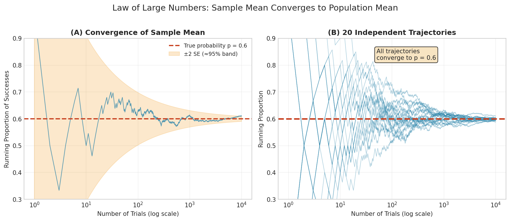
Fig. 4 Law of Large Numbers in action. (A) A single sequence of coin flips converges toward \(p = 0.6\), with the ±2 SE band shrinking as \(n\) increases. (B) Twenty independent trajectories all converge to the same limit, demonstrating that \(\bar{X}_n \xrightarrow{P} \mu\) regardless of the particular sample path.

Central Limit Theorem (Lindeberg–Lévy): If in addition \(\text{Var}(X_1) = \sigma^2 < \infty\), then

\[\frac{\sqrt{n}\,(\bar{X}_n - \mu)}{\sigma} \xrightarrow{d} \mathcal{N}(0,1).\]

Unless specified otherwise, “Law of Large Numbers” will refer to the weak version (convergence in probability).

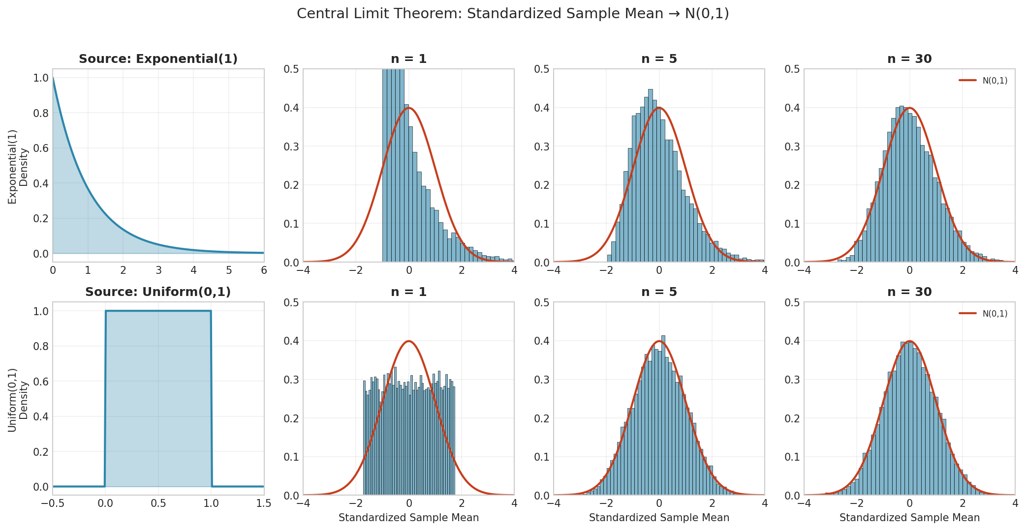
Fig. 5 Central Limit Theorem demonstration. Regardless of the source distribution (top row: Exponential; bottom row: Uniform), the standardized sample mean converges to \(N(0,1)\) as \(n\) increases. At \(n = 1\), the shape matches the source; by \(n = 30\), both are nearly indistinguishable from the normal curve (red).

Common Limits in Probability

Several limits recur throughout probability and statistics:

\[\lim_{n \to \infty} \left(1 + \frac{x}{n}\right)^n = e^x, \qquad \lim_{n \to \infty} \left(1 - \frac{\lambda}{n}\right)^n = e^{-\lambda}.\]

These motivate classical approximations. For example, if \(X_n \sim \text{Binomial}(n, \lambda/n)\) then \(X_n \xrightarrow{d} \text{Poisson}(\lambda)\) as \(n \to \infty\).

Quick Check ✓

Before proceeding, verify you understand:

1. What is the difference between \(X_n \xrightarrow{P} X\) and \(X_n \xrightarrow{a.s.} X\)?

2. Can a sequence converge in distribution but not in probability? (Hint: \(X_n \sim \mathcal{N}(0,1)\) i.i.d.)

3. Evaluate: \(\lim_{n \to \infty} \left(1 - \frac{2}{n}\right)^n\)

4. If \(f(n) = 5n^2 + 3n\), what is \(f(n)\) in big-O notation?

Answers: (1) Probability convergence means high probability of being close; almost sure convergence means pathwise convergence with probability 1 and is stronger. (2) Yes. The i.i.d. normal example has constant distribution in \(n\) but does not converge in probability to any random variable. (3) \(e^{-2} \approx 0.135\). (4) \(O(n^2)\).

With these mathematical tools in hand, we are ready to explore interpretations of probability and their profound philosophical and practical implications.

Interpretations of Probability

All modern approaches to probability and statistics—frequentist, Bayesian, and likelihoodist—accept Kolmogorov’s axioms as the mathematical foundation, established in his 1933 monograph Grundbegriffe der Wahrscheinlichkeitsrechnung (Foundations of the Theory of Probability). [1] While everyone agrees on these mathematical rules, there is profound disagreement about what probability actually represents. The main interpretations fall into two broad categories: objective (probability as a feature of the world) and epistemic (probability as a degree of knowledge or belief). These different interpretations have enormous practical consequences for how we conduct statistical inference and computational analysis.

[1]

Specialized domains like quantum mechanics use modified probability axioms for non-commuting observables, and researchers have explored generalizations like imprecise probability. These are extensions or domain-specific adaptations rather than rejections of the classical framework, which remains universal for statistical data science.

Objective Interpretations: Probability as Physical Reality

Objective interpretations treat probability as a property of the physical world, independent of any observer’s knowledge or beliefs.

A. Frequentist Interpretation

The frequentist interpretation defines probability as the long-run relative frequency of an event in repeated trials under identical conditions.

Core Idea: If we repeat a random experiment many times, the probability of an event \(E\) equals the limiting proportion of trials in which \(E\) occurs:

\[P(E) = \lim_{n \to \infty} \frac{\text{Number of times } E \text{ occurs in } n \text{ trials}}{n}\]

For example, saying “the probability of heads is 0.5” means that if we flip a fair coin infinitely many times, approximately half will be heads. This limiting frequency is an objective property of the coin, not dependent on anyone’s beliefs.

Connection to Law of Large Numbers: The frequentist interpretation is closely tied to the mathematical Law of Large Numbers, which states that the sample mean of independent, identically distributed (i.i.d.) random variables converges to the population mean as sample size increases. For a coin with true probability \(p\) of heads, if \(X_i = 1\) for heads and \(X_i = 0\) for tails, then:

\[\bar{X}_n = \frac{1}{n}\sum_{i=1}^{n} X_i \xrightarrow{P} p \quad \text{as } n \to \infty\]

Strengths:

• Objective: Doesn’t depend on subjective beliefs or opinions

• Empirically verifiable: Can be tested through repeated experimentation

• Clear operational meaning: Provides concrete, observable interpretation

• Mathematical foundation: Connects directly to limit theorems in probability theory

Limitations:

• Non-repeatable events: Cannot assign probabilities to unique events (e.g., “What is the probability that this specific patient will survive surgery?” or “What is the probability that the Higgs boson exists?”). Frequentists handle such cases by positing a repeatable data-generating mechanism (e.g., patients with similar characteristics), but they resist assigning probabilities to the truth values of fixed parameters or one-time hypotheses.

• Infinite sequence required: The limit as \(n \to \infty\) is a mathematical idealization that can never be physically realized

• Circularity: How many trials are “enough” to approximate the limiting frequency? We need probability to answer this question.

• Fixed parameters: Cannot treat population parameters as random, making statements like “the probability that \(\mu > 0\)” meaningless in the frequentist framework

Example 💡: Coin Flipping Simulation

Given: A biased coin with true probability \(p = 0.6\) of heads.

Find: Demonstrate convergence of relative frequency to true probability.

Mathematical approach:

The relative frequency after \(n\) flips is \(\hat{p}_n = \frac{1}{n}\sum_{i=1}^{n} X_i\) where \(X_i \sim \text{Bernoulli}(0.6)\). By the Law of Large Numbers:

\[\hat{p}_n \xrightarrow{P} 0.6 \quad \text{as } n \to \infty\]

The standard error decreases as \(\text{SE}(\hat{p}_n) = \sqrt{p(1-p)/n} = \sqrt{0.24/n}\).

Python implementation:

import numpy as np

np.random.seed(42)

# True probability
p_true = 0.6

# Simulate coin flips
n_max = 10000
flips = np.random.binomial(1, p_true, n_max)

# Compute cumulative relative frequency
cumsum = np.cumsum(flips)
n_trials = np.arange(1, n_max + 1)
rel_freq = cumsum / n_trials

# Compute standard error bounds
se = np.sqrt(p_true * (1 - p_true) / n_trials)

# Print convergence at key milestones
milestones = [10, 100, 1000, 10000]
print("Convergence of relative frequency to true probability:")
print(f"{'n':>6s} | {'Rel. Freq.':>12s} | {'Std. Error':>12s} | {'Distance':>12s}")
print("-" * 50)
for n in milestones:
    idx = n - 1
    distance = abs(rel_freq[idx] - p_true)
    print(f"{n:6d} | {rel_freq[idx]:12.6f} | {se[idx]:12.6f} | {distance:12.6f}")

Result:

Convergence of relative frequency to true probability:
     n |  Rel. Freq. |  Std. Error |     Distance
--------------------------------------------------
    10 |     0.600000 |     0.154919 |     0.000000
   100 |     0.640000 |     0.048990 |     0.040000
  1000 |     0.608000 |     0.015492 |     0.008000
 10000 |     0.601300 |     0.004899 |     0.001300

After 10,000 flips, the relative frequency (0.6013) is within 0.0013 of the true probability, and the standard error has decreased to approximately 0.005. This demonstrates the Law of Large Numbers in action, though note that even with 10,000 trials, we haven’t reached the theoretical limit—we’ve only approximated it.

B. Propensity Interpretation

The propensity interpretation, developed by philosopher Karl Popper in 1957, treats probability as a physical disposition or tendency of a system to produce certain outcomes.

Core Idea: Probability is an objective property of a chance setup—a “propensity” or physical tendency that exists even for single trials. A radioactive atom has a propensity of 0.1 to decay in the next hour; this is neither a long-run frequency (which would require many identical atoms) nor a belief, but a real physical property of this particular atom.

Strengths:

• Single-case application: Can meaningfully assign probabilities to unique, non-repeatable events

• Maintains objectivity: Probability remains a feature of the world, not dependent on beliefs

• Explains convergence: Long-run frequencies stabilize because underlying propensities determine outcomes

• Quantum mechanics: Provides a natural interpretation for inherently stochastic quantum processes

Limitations:

• Conceptual vagueness: What exactly is a “propensity”? How do we measure or verify it independently of frequencies?

• Empirical collapse: In practice, propensities are estimated from frequencies, potentially reducing to frequentism

• Theoretical paradoxes: Humphreys’ Paradox shows that propensity interpretations face logical difficulties when applying Bayes’ theorem

• Limited adoption: Rarely used in practical statistical analysis despite philosophical appeal

Epistemic Interpretations: Probability as Degree of Belief

Epistemic interpretations treat probability not as a property of the external world, but as a quantification of uncertainty, knowledge, or degree of belief about propositions.

A. Subjective (Bayesian) Interpretation

The subjective Bayesian interpretation defines probability as a rational agent’s degree of belief or confidence in a proposition, given their available information and prior knowledge.

Core Idea: Probability quantifies how strongly someone believes a proposition is true. Different individuals with different information can rationally assign different probabilities to the same event. Italian mathematician Bruno de Finetti famously declared: “Probability does not exist” as an objective feature of reality—only subjective degrees of belief constrained by the rationality requirements of coherence exist.

This interpretation was developed independently by Frank Ramsey (1926), Bruno de Finetti (1937), and Leonard Savage (1954) in the early to mid-20th century, forming the foundation of modern Bayesian statistics.

The Dutch Book Argument for Coherence

How do we know subjective probabilities should follow Kolmogorov’s axioms? The Dutch Book argument provides the justification: If your probability assignments violate the axioms, someone can construct a set of bets (a “Dutch book”) that guarantees you lose money regardless of which outcomes occur. Rational agents should therefore maintain coherent beliefs that satisfy the probability axioms.

For example, suppose you assign probabilities that violate additivity for disjoint events \(A\) and \(B\):

• \(P(A) = 0.6\) (you’ll pay $0.60 for a bet that pays $1 if \(A\) occurs)

• \(P(B) = 0.5\) (you’ll pay $0.50 for a bet that pays $1 if \(B\) occurs)

• \(P(A \cup B) = 0.9\) (you’ll accept $0.90 to provide a bet that pays $1 if \(A\) or \(B\) occurs)

If \(A\) and \(B\) are disjoint, these probabilities violate Axiom 3: they should satisfy \(P(A \cup B) = P(A) + P(B) = 1.1\), not 0.9. Since your \(P(A \cup B) = 0.9 < 1.1\), you’ve undervalued the combined event.

A clever opponent exploits this by:

1. Buying from you the bet on \(A \cup B\) for $0.90 (you receive $0.90, must pay $1 if \(A\) or \(B\) occurs)

2. Selling to you the bet on \(A\) for $0.60 (you pay $0.60, receive $1 if \(A\) occurs)

3. Selling to you the bet on \(B\) for $0.50 (you pay $0.50, receive $1 if \(B\) occurs)

Your net position:

• Upfront cash flow: \(+0.90 - 0.60 - 0.50 = -0.20\) (you lose $0.20 immediately)

• If \(A\) occurs (but not \(B\)): Pay $1 on combined bet, receive $1 on \(A\) bet = net $0, total loss = $0.20

• If \(B\) occurs (but not \(A\)): Pay $1 on combined bet, receive $1 on \(B\) bet = net $0, total loss = $0.20

• If neither occurs: Pay $0 on all bets, total loss = $0.20

You lose $0.20 guaranteed, regardless of outcome—this is the Dutch Book. Maintaining coherent probabilities that satisfy Kolmogorov’s axioms prevents such exploitation.

Strengths:

• Universal applicability: Can assign probabilities to any proposition—hypotheses, parameters, future events, past events we’re uncertain about

• Incorporates prior information: Naturally combines existing knowledge with new data via Bayes’ theorem

• Direct probability statements: Can say “there is a 95% probability that :math:`mu > 0$” directly

• Handles unique events: Natural framework for one-time events like “Will it rain tomorrow?” or “Is this hypothesis true?”

• Coherent updating: Bayes’ theorem provides the unique coherent way to update beliefs given new evidence

Limitations:

• Prior dependence: Requires specifying a prior distribution, which may be subjective or controversial

• Prior sensitivity: With limited data, conclusions can be sensitive to prior choice

• Subjectivity concerns: Critics argue personal beliefs have no place in scientific inference

• Computational demands: Bayesian inference often requires intensive computation (MCMC, numerical integration)

• Communication challenges: Different priors can lead to different conclusions, complicating scientific consensus

Example 💡: Medical Diagnosis with Bayesian Updating

Given: A rare disease affects 1% of the population. A diagnostic test has 95% sensitivity (true positive rate) and 90% specificity (true negative rate). A patient tests positive.

Find: The probability the patient has the disease, and demonstrate Bayesian updating.

Mathematical approach:

Let \(D\) = patient has disease, \(T^+\) = positive test result. We know:

• Prior: \(P(D) = 0.01\), \(P(D^c) = 0.99\)

• Likelihood: \(P(T^+ \mid D) = 0.95\) (sensitivity), \(P(T^+ \mid D^c) = 0.10\) (false positive rate = 1 - specificity)

By Bayes’ theorem:

\[P(D \mid T^+) = \frac{P(T^+ \mid D) \cdot P(D)}{P(T^+)}\]

where the marginal likelihood is:

\[P(T^+) = P(T^+ \mid D) \cdot P(D) + P(T^+ \mid D^c) \cdot P(D^c) = 0.95(0.01) + 0.10(0.99) = 0.1085\]

Therefore:

\[P(D \mid T^+) = \frac{0.95 \times 0.01}{0.1085} = \frac{0.0095}{0.1085} \approx 0.0876\]

Interpretation: Despite the positive test, there’s only an 8.76% probability the patient has the disease! This counterintuitive result occurs because the disease is rare (low prior) and the false positive rate is non-negligible.

Python implementation:

def bayesian_diagnostic(prior_disease, sensitivity, specificity):
    """
    Compute posterior probability of disease given positive test.

    Parameters
    ----------
    prior_disease : float
        Prior probability of having the disease, P(D)
    sensitivity : float
        True positive rate, P(T+ | D)
    specificity : float
        True negative rate, P(T- | D^c)

    Returns
    -------
    dict
        Dictionary with prior, likelihood components, and posterior
    """
    # False positive rate
    fpr = 1 - specificity

    # Marginal likelihood P(T+)
    p_test_pos = sensitivity * prior_disease + fpr * (1 - prior_disease)

    # Posterior by Bayes' theorem
    posterior = (sensitivity * prior_disease) / p_test_pos

    return {
        'prior': prior_disease,
        'likelihood_disease': sensitivity,
        'likelihood_healthy': fpr,
        'marginal_likelihood': p_test_pos,
        'posterior': posterior
    }

# Compute for our scenario
result = bayesian_diagnostic(prior_disease=0.01, sensitivity=0.95, specificity=0.90)

print(f"Prior probability of disease: {result['prior']:.4f}")
print(f"Marginal probability of positive test: {result['marginal_likelihood']:.4f}")
print(f"Posterior probability of disease | positive test: {result['posterior']:.4f}")

# Compute update factor (Bayes factor)
bayes_factor = result['likelihood_disease'] / result['likelihood_healthy']
print(f"\nBayes factor (evidence strength): {bayes_factor:.2f}")
print(f"Posterior odds: {result['posterior']/(1-result['posterior']):.4f}")
print(f"Prior odds: {result['prior']/(1-result['prior']):.4f}")

Result:

Prior probability of disease: 0.0100
Marginal probability of positive test: 0.1085
Posterior probability of disease | positive test: 0.0876

Bayes factor (evidence strength): 9.50
Posterior odds: 0.0960
Prior odds: 0.0101

The positive test increases our degree of belief in the disease from 1% to 8.76%—a 9.5-fold increase in odds. However, because the prior probability was so low, the posterior remains below 10%. This example illustrates the crucial role of prior information in Bayesian inference and the often counterintuitive nature of diagnostic reasoning.

B. Logical and Objective Bayesian Interpretations

These interpretations attempt to remove or minimize subjectivity from Bayesian probability by using formal principles to construct priors.

Logical Interpretation (Keynes, Carnap): Probability is a logical relation between propositions, analogous to how deductive logic provides certain relations. The probability \(P(H \mid E)\) represents the degree to which evidence \(E\) logically supports hypothesis \(H\), independent of any particular person’s beliefs.

Objective Bayesian Interpretation (Jaynes, Jeffreys): Use formal principles like maximum entropy or symmetry requirements to construct “non-informative” or “reference” priors that represent ignorance in a principled, objective way. The goal is priors that any rational person would agree on given the same state of information.

For example, Jeffreys’ prior uses the Fisher information (discussed in Chapter 3) to define a prior invariant under reparameterization:

\[\pi(\theta) \propto \sqrt{\det I(\theta)}\]

where \(I(\theta)\) is the Fisher information matrix.

Key Insight: Even these “objective” approaches yield probabilities conditional on assumptions (choice of reference class, parameterization, symmetry principles). They represent conditional objectivity—objective given the framework, but the framework itself involves choices.

Summary of Interpretations

The landscape of probability interpretations:

Interpretation	Type	Core Idea	Key Limitation
Frequentist	Objective	Long-run relative frequency	Cannot handle unique events or parameters
Propensity	Objective	Physical disposition/tendency	Conceptually vague, hard to measure
Subjective Bayesian	Epistemic	Personal degree of belief	Requires subjective priors
Logical	Epistemic	Evidential support relation	Still requires assumptions
Objective Bayesian	Epistemic	Principled ignorance	“Objectivity” is conditional

Key Insight 🔑

All interpretations agree on the mathematical rules (Kolmogorov’s axioms) but profoundly disagree on what probability means. This philosophical difference has enormous practical implications for statistical inference, computational methods, and how we interpret results in data science applications.

Statistical Inference Paradigms

Statistical inference is the process of drawing conclusions about populations, processes, or hypotheses from observed data. Different interpretations of probability naturally lead to radically different approaches to inference. We examine three major paradigms that shape modern statistical practice.

Frequentist Inference (Classical Approach)

Frequentist inference aligns with the frequentist interpretation of probability. Parameters are fixed but unknown constants; randomness enters only through the sampling process. Inference focuses on procedures that have good long-run frequency properties across repeated samples.

Key Principles

1. Parameters are fixed: Population quantities like the mean \(\mu\) or proportion \(p\) have true, fixed values—they are not random variables.

2. Data are random: The sample \(X_1, X_2, \ldots, X_n\) is randomly drawn from a population; the randomness is in the sampling process.

3. Procedures have frequency properties: We evaluate inference methods by how they perform across hypothetical repeated samples from the same population.

Core Methods

A. Point Estimation

A point estimator \(\hat{\theta}\) is a function of the data used to estimate parameter \(\theta\). We evaluate estimators by their properties across repeated samples:

• Unbiased: \(E[\hat{\theta}] = \theta\) (on average, the estimator equals the true parameter)

• Consistent: \(\hat{\theta} \xrightarrow{P} \theta\) as \(n \to \infty\) (converges to truth with more data)

• Efficient: Among unbiased estimators, has minimum variance

The maximum likelihood estimator (MLE) is frequently used because it has optimal asymptotic properties:

\[\hat{\theta}_{\text{MLE}} = \arg\max_{\theta} L(\theta; \text{data}) = \arg\max_{\theta} \prod_{i=1}^{n} f(x_i \mid \theta)\]

where \(f(x \mid \theta)\) is the probability density/mass function of the data given \(\theta\).

B. Confidence Intervals

A \(100(1-\alpha)\%\) confidence interval is an interval \([\hat{\theta}_L, \hat{\theta}_U]\) constructed so that if we repeated the sampling procedure many times and computed the interval each time, approximately \(100(1-\alpha)\%\) of those intervals would contain the true parameter \(\theta\).

Mathematically:

\[P(\hat{\theta}_L(\mathbf{X}) < \theta < \hat{\theta}_U(\mathbf{X})) = 1 - \alpha\]

where the probability is over the random sample \(\mathbf{X} = (X_1, \ldots, X_n)\).

Critical interpretation point: The parameter \(\theta\) is fixed—it’s not random and doesn’t have a probability distribution. The interval \((\hat{\theta}_L, \hat{\theta}_U)\) is random because it depends on the random sample. Once we observe a specific sample and compute a specific interval, that interval either contains \(\theta\) or it doesn’t—we cannot say “there is a 95% probability \(\theta\) is in this specific interval” in the frequentist framework.

C. Hypothesis Testing

Test a null hypothesis \(H_0\) against an alternative hypothesis \(H_a\) using the following procedure:

1. Choose a test statistic \(T(\mathbf{X})\) that measures deviation from \(H_0\)

2. Determine the sampling distribution of \(T\) assuming \(H_0\) is true

3. Calculate the p-value: \(P(T \geq t_{\text{obs}} \mid H_0)\) where \(t_{\text{obs}}\) is the observed test statistic

4. Compare to a pre-specified significance level \(\alpha\) (commonly 0.05)

Interpretation of p-value: The p-value is the probability of observing a test statistic as extreme or more extreme than what we observed, if the null hypothesis were true. It is not the probability that \(H_0\) is true, nor is it the probability that \(H_a\) is false.

Mathematically: \(p = P(\text{Data as or more extreme} \mid H_0 \text{ true})\)

Not: \(P(H_0 \text{ true} \mid \text{Data})\) ← This would be the Bayesian posterior probability.

Neyman-Pearson vs. Fisherian Approaches

Within frequentist inference, two sub-schools have different emphases:

Neyman-Pearson Framework (Jerzy Neyman, Egon Pearson, 1930s):

• Formalize hypothesis testing as a decision problem

• Control Type I error \(\alpha = P(\text{Reject } H_0 \mid H_0 \text{ true})\) and Type II error \(\beta = P(\text{Fail to reject } H_0 \mid H_0 \text{ false})\)

• Power \(= 1 - \beta = P(\text{Reject } H_0 \mid H_a \text{ true})\)

• Optimize test procedures to maximize power for fixed \(\alpha\)

• View testing as leading to a binary decision: reject or fail to reject

Fisherian Framework (Ronald Fisher, 1920s-1950s):

• Emphasize the p-value as a continuous measure of evidence against \(H_0\)

• Less rigid about fixed \(\alpha\) levels; p-value interpreted as strength of evidence

• Focus on the likelihood function as containing all information data provide about parameters

• View testing as evidence assessment rather than decision-making

• More flexible, less formalized than Neyman-Pearson

Modern practice often blends both approaches, sometimes inconsistently.

Example 💡: Two-Sample T-Test (Frequentist Framework)

Given: Two groups of measurements. Group A (treatment): [5.1, 5.5, 5.3, 5.7, 5.4, 5.6] and Group B (control): [4.8, 4.9, 5.0, 4.7, 4.9, 5.1].

Find: Test whether the treatment increases the mean response using a one-sided t-test at \(\alpha = 0.05\).

Mathematical approach:

• Null hypothesis: \(H_0: \mu_A = \mu_B\) (or \(\mu_A - \mu_B = 0\))

• Alternative: \(H_a: \mu_A > \mu_B\) (treatment increases mean)

• Test statistic (assuming equal variances):

\[t = \frac{\bar{X}_A - \bar{X}_B}{s_p \sqrt{1/n_A + 1/n_B}}\]

where \(s_p\) is the pooled standard deviation:

\[s_p = \sqrt{\frac{(n_A - 1)s_A^2 + (n_B - 1)s_B^2}{n_A + n_B - 2}}\]

Under \(H_0\), \(t\) follows a t-distribution with \(n_A + n_B - 2\) degrees of freedom.

Python implementation:

from scipy import stats
import numpy as np

# Data
group_a = np.array([5.1, 5.5, 5.3, 5.7, 5.4, 5.6])
group_b = np.array([4.8, 4.9, 5.0, 4.7, 4.9, 5.1])

# Summary statistics
n_a, n_b = len(group_a), len(group_b)
mean_a, mean_b = np.mean(group_a), np.mean(group_b)
std_a, std_b = np.std(group_a, ddof=1), np.std(group_b, ddof=1)

# Pooled standard deviation
s_p = np.sqrt(((n_a - 1) * std_a**2 + (n_b - 1) * std_b**2) / (n_a + n_b - 2))

# Test statistic
t_stat = (mean_a - mean_b) / (s_p * np.sqrt(1/n_a + 1/n_b))

# Degrees of freedom
df = n_a + n_b - 2

# One-sided p-value (alternative: mean_a > mean_b)
p_value = stats.t.sf(t_stat, df)

# Using scipy's built-in function with matching assumptions
t_stat_scipy, p_value_scipy = stats.ttest_ind(
    group_a, group_b, equal_var=True, alternative='greater'
)

print(f"Sample means: A = {mean_a:.3f}, B = {mean_b:.3f}")
print(f"Mean difference: {mean_a - mean_b:.3f}")
print(f"Pooled SD: {s_p:.3f}")
print(f"Test statistic: t = {t_stat:.3f}")
print(f"Degrees of freedom: {df}")
print(f"One-sided p-value: {p_value:.4f}")
print(f"SciPy p-value (verification): {p_value_scipy:.4f}")
print(f"\nDecision at α=0.05: {'Reject H₀' if p_value < 0.05 else 'Fail to reject H₀'}")

# 95% confidence interval for difference in means
t_critical = stats.t.ppf(0.975, df)
se_diff = s_p * np.sqrt(1/n_a + 1/n_b)
ci_lower = (mean_a - mean_b) - t_critical * se_diff
ci_upper = (mean_a - mean_b) + t_critical * se_diff
print(f"\n95% CI for mean difference: [{ci_lower:.3f}, {ci_upper:.3f}]")

Result:

Sample means: A = 5.433, B = 4.900
Mean difference: 0.533
Pooled SD: 0.278
Test statistic: t = 3.319
Degrees of freedom: 10
One-sided p-value: 0.0039
SciPy p-value (verification): 0.0039

Decision at α=0.05: Reject H₀

95% CI for mean difference: [0.276, 0.791]

Frequentist interpretation: “If the null hypothesis (no treatment effect) were true, we would observe a difference in means as large as 0.533 or larger in only 0.39% of repeated samples. This provides strong evidence against \(H_0\), so we reject it at \(\alpha = 0.05\).”

What we do NOT say: “There is a 99.61% probability the treatment works” or “There is a 0.39% probability the null is true.” In the frequentist framework, hypotheses are not random—they are either true or false. Only data have probability distributions.

Confidence interval interpretation: “If we repeated this study many times and calculated 95% CIs each time, approximately 95% of those intervals would contain the true mean difference.” Once we have a specific interval [0.276, 0.791], it either contains the true difference or it doesn’t—we don’t assign a probability.

Strengths and Limitations of Frequentist Inference

Strengths:

• Objective: No need for subjective prior beliefs about parameters

• Well-established: Extensive theory with clear guarantees on error rates and convergence properties

• Regulatory acceptance: Standard in clinical trials, FDA submissions, and scientific publications

• Computational simplicity: Many standard procedures have closed-form solutions or simple algorithms

• Long track record: Decades of successful application across sciences

Limitations:

• No probability statements about parameters: Cannot say “probability that \(\mu > 0$" since :math:\)mu` is fixed

• Confidence intervals often misinterpreted: Frequently confused with Bayesian credible intervals

• P-values widely misunderstood: Not the probability of hypothesis, often leads to binary thinking

• Cannot incorporate prior information formally: Expert knowledge must be handled informally

• Stopping rules matter: Results depend on whether you planned to sample \(n\) observations or sample until seeing \(k\) events (violates likelihood principle)

• Counterintuitive results: Optional stopping and sequential testing can produce seemingly paradoxical results

Bayesian Inference

Bayesian inference treats all unknowns as random variables with probability distributions. It aligns with the subjective (or objective Bayesian) interpretation where probability represents degree of belief or uncertainty.

Key Principles

1. Parameters are random: We assign probability distributions to unknown parameters representing our uncertainty

2. Update beliefs with data: Bayes’ theorem mechanically converts prior beliefs into posterior beliefs after observing data

3. Probability as belief: We make direct probability statements about anything unknown—parameters, hypotheses, predictions

Bayes’ Theorem

The foundation of all Bayesian inference is Bayes’ theorem applied to parameters:

\[P(\theta \mid \mathbf{X}) = \frac{P(\mathbf{X} \mid \theta) \cdot P(\theta)}{P(\mathbf{X})}\]

Or more intuitively:

\[\underbrace{P(\theta \mid \mathbf{X})}_{\text{Posterior}} = \frac{\overbrace{P(\mathbf{X} \mid \theta)}^{\text{Likelihood}} \times \overbrace{P(\theta)}^{\text{Prior}}}{\underbrace{P(\mathbf{X})}_{\text{Evidence}}}\]

Where:

• Prior \(P(\theta)\): Our belief about \(\theta\) before seeing data, representing prior knowledge

• Likelihood \(P(\mathbf{X} \mid \theta)\): How probable the observed data are for each parameter value

• Posterior \(P(\theta \mid \mathbf{X})\): Our updated belief about \(\theta\) after incorporating the data

• Evidence (marginal likelihood) \(P(\mathbf{X}) = \int P(\mathbf{X} \mid \theta) P(\theta) \, d\theta\): Normalizing constant ensuring posterior integrates to 1

Since the evidence doesn’t depend on \(\theta\), we often write:

\[P(\theta \mid \mathbf{X}) \propto P(\mathbf{X} \mid \theta) \cdot P(\theta)\]

The posterior is proportional to likelihood times prior.

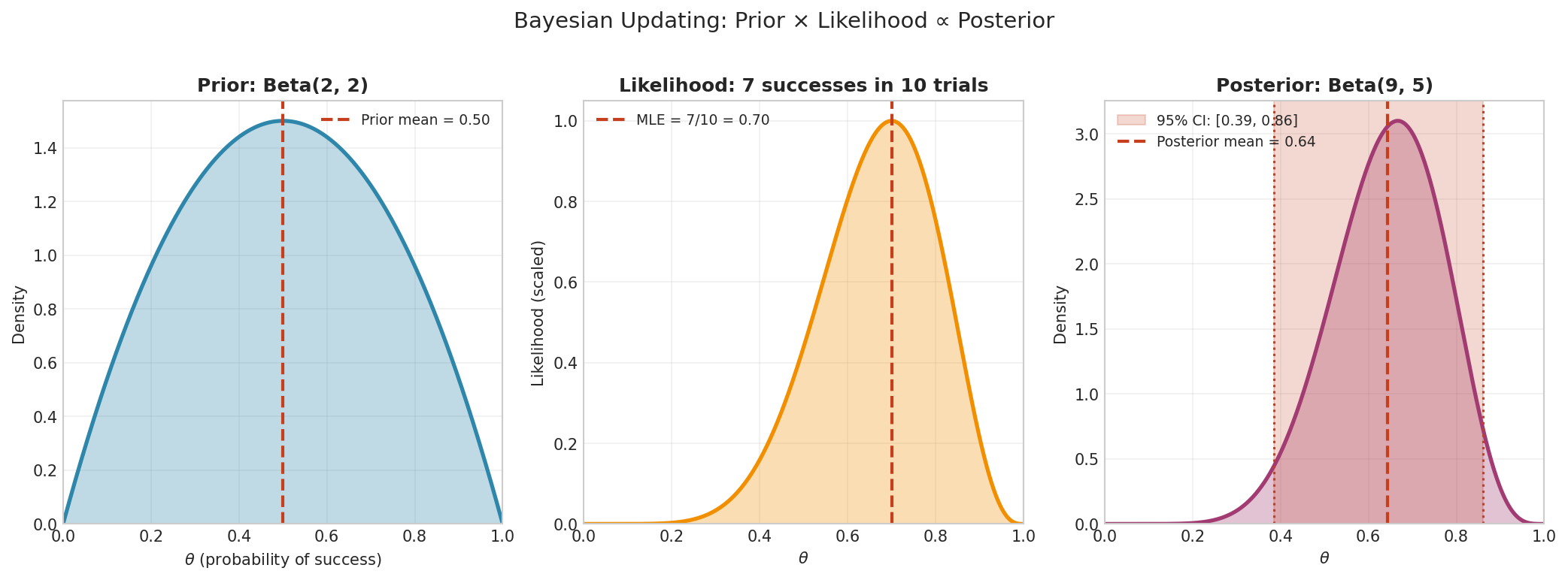
Fig. 6 Bayesian updating with conjugate priors. Starting with a Beta(2, 2) prior (mild belief that \(\theta \approx 0.5\)), we observe 7 successes in 10 trials. The likelihood peaks at the MLE \(\hat{\theta} = 0.7\). The posterior Beta(9, 5) is a compromise between prior and data, with a 95% credible interval of [0.39, 0.86].

Core Methods

A. Point Estimation

Multiple Bayesian point estimates exist, each with different optimality properties:

• Posterior mean: \(\hat{\theta} = E[\theta \mid \mathbf{X}] = \int \theta \, P(\theta \mid \mathbf{X}) \, d\theta\) (minimizes squared error loss)

• Posterior mode (MAP): \(\hat{\theta} = \arg\max_{\theta} P(\theta \mid \mathbf{X})\) (maximizes posterior density)

• Posterior median: 50th percentile of posterior (minimizes absolute error loss)

B. Interval Estimation (Credible Intervals)

A \(100(1-\alpha)\%\) credible interval (or posterior interval) is an interval \([L, U]\) such that:

\[P(L < \theta < U \mid \mathbf{X}) = 1 - \alpha\]

Interpretation: There is a \(100(1-\alpha)\%\) probability that \(\theta\) lies in this interval, given the data and prior. This is a direct probability statement about the parameter!

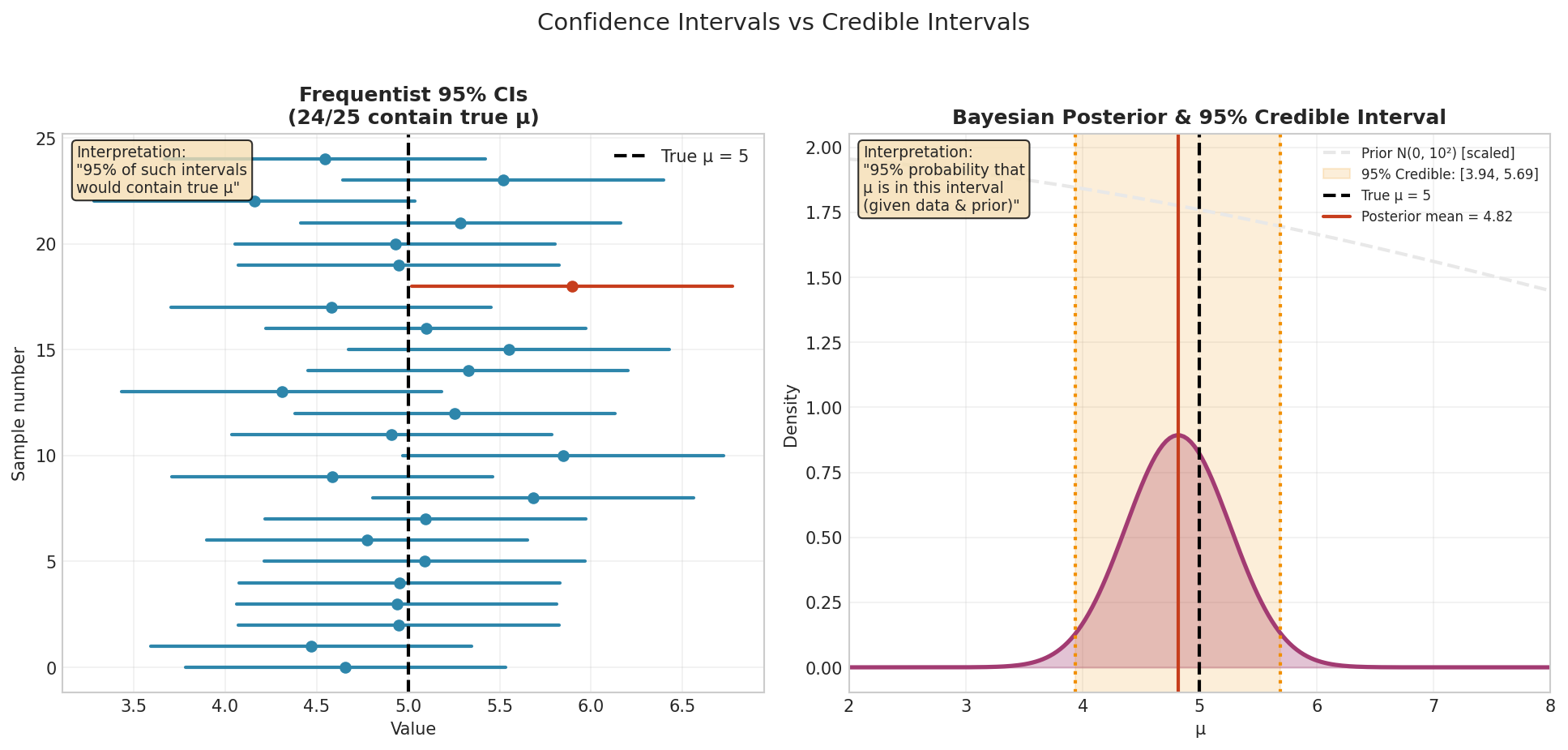
Fig. 7 Frequentist vs Bayesian interval interpretation. Left: Each of 25 samples yields a different 95% CI; approximately 95% contain the true \(\mu = 5\) (blue), while ~5% miss (red). The parameter is fixed; the intervals are random. Right: A single Bayesian analysis produces one posterior distribution; the 95% credible interval has a direct probability interpretation: “Given the data and prior, there is 95% probability \(\mu\) lies in this interval.”

Common types: * Equal-tailed interval: \(\alpha/2\) probability in each tail * Highest posterior density (HPD) interval: Shortest interval containing \(1-\alpha\) probability mass

C. Hypothesis Testing and Model Comparison

Posterior probabilities: Directly compute \(P(H_0 \mid \mathbf{X})\) and \(P(H_a \mid \mathbf{X})\).

Bayes factors: Compare evidence for competing hypotheses/models:

\[\text{BF}_{10} = \frac{P(\mathbf{X} \mid H_1)}{P(\mathbf{X} \mid H_0)} = \frac{\int P(\mathbf{X} \mid \theta, H_1) P(\theta \mid H_1) \, d\theta}{\int P(\mathbf{X} \mid \theta, H_0) P(\theta \mid H_0) \, d\theta}\]

The Bayes factor quantifies how many times more likely the data are under \(H_1\) compared to \(H_0\). By Bayes’ theorem:

\[\underbrace{\frac{P(H_1 \mid \mathbf{X})}{P(H_0 \mid \mathbf{X})}}_{\text{Posterior odds}} = \underbrace{\text{BF}_{10}}_{\text{Bayes factor}} \times \underbrace{\frac{P(H_1)}{P(H_0)}}_{\text{Prior odds}}\]

Interpretation scale (Kass & Raftery, 1995): * BF < 1: Evidence for \(H_0\) * 1-3: Barely worth mentioning * 3-10: Substantial evidence for \(H_1\) * 10-100: Strong evidence * > 100: Decisive evidence

The Role of Priors

Choosing a prior is crucial and sometimes controversial. Common approaches:

• Informative priors: Based on previous studies, expert knowledge, physical constraints, or theoretical considerations. Example: If measuring human height, prior might be \(N(170, 20^2)\) cm.

• Weakly informative priors: Provide gentle regularization without dominating data. Example: \(N(0, 10^2)\) for a standardized effect size.

• Non-informative priors: Attempt to express ignorance objectively: - Uniform prior: \(p(\theta) \propto 1\) (equal belief in all values) - Jeffreys prior: \(p(\theta) \propto \sqrt{\det I(\theta)}\) (invariant under reparameterization) - Reference priors: Maximize expected information gain from data

Key insight: With large sample sizes, the likelihood dominates and different reasonable priors yield similar posteriors. Prior choice matters most with limited data.

Example 💡: Bayesian Estimation of Binomial Proportion

Given: We observe 8 successes in 10 trials. Estimate the success probability \(p\).

Find: Posterior distribution of \(p\) under uniform and informative priors.

Mathematical approach:

• Likelihood: \(P(y=8 \mid p, n=10) = \binom{10}{8} p^8 (1-p)^2\)

• Prior 1 (uniform): \(p \sim \text{Beta}(1, 1)\) (equivalent to uniform on [0,1])

• Prior 2 (informative): \(p \sim \text{Beta}(5, 5)\) (skeptical, centered at 0.5)

With a Beta prior \(\text{Beta}(\alpha, \beta)\) and binomial likelihood, the posterior is:

\[p \mid y \sim \text{Beta}(\alpha + y, \beta + n - y)\]

Uniform prior posterior:

\[p \mid y=8 \sim \text{Beta}(1+8, 1+2) = \text{Beta}(9, 3)\]

Informative prior posterior:

\[p \mid y=8 \sim \text{Beta}(5+8, 5+2) = \text{Beta}(13, 7)\]

Python implementation:

from scipy import stats
import numpy as np

# Data
y, n = 8, 10

# Priors
prior_uniform = stats.beta(1, 1)  # Beta(1,1) = Uniform(0,1)
prior_inform = stats.beta(5, 5)   # Skeptical prior

# Posteriors (conjugate update)
posterior_uniform = stats.beta(1 + y, 1 + (n - y))  # Beta(9, 3)
posterior_inform = stats.beta(5 + y, 5 + (n - y))   # Beta(13, 7)

# MLE for comparison
p_mle = y / n

# Posterior summaries
def summarize_beta(dist, name):
    mean = dist.mean()
    # Mode formula (α-1)/(α+β-2) valid only for α,β > 1
    if dist.args[0] > 1 and dist.args[1] > 1:
        mode = (dist.args[0] - 1) / (dist.args[0] + dist.args[1] - 2)
    else:
        mode = np.nan
    median = dist.median()
    ci = dist.interval(0.95)
    print(f"\n{name}:")
    print(f"  Mean: {mean:.4f}")
    print(f"  Mode: {mode:.4f}")
    print(f"  Median: {median:.4f}")
    print(f"  95% Credible Interval: [{ci[0]:.4f}, {ci[1]:.4f}]")
    return mean, ci

print("="*50)
print("BAYESIAN BINOMIAL PROPORTION ESTIMATION")
print("="*50)
print(f"Observed: {y} successes in {n} trials")
print(f"MLE (Frequentist): {p_mle:.4f}")

mean_u, ci_u = summarize_beta(posterior_uniform, "Posterior (Uniform Prior)")
mean_i, ci_i = summarize_beta(posterior_inform, "Posterior (Informative Prior)")

# Probability that p > 0.5
prob_gt_half_u = 1 - posterior_uniform.cdf(0.5)
prob_gt_half_i = 1 - posterior_inform.cdf(0.5)

print(f"\nP(p > 0.5 | data, uniform prior): {prob_gt_half_u:.4f}")
print(f"P(p > 0.5 | data, informative prior): {prob_gt_half_i:.4f}")

Result:

==================================================
BAYESIAN BINOMIAL PROPORTION ESTIMATION
==================================================
Observed: 8 successes in 10 trials
MLE (Frequentist): 0.8000

Posterior (Uniform Prior):
  Mean: 0.7500
  Mode: 0.8000
  Median: 0.7528
  95% Credible Interval: [0.4822, 0.9451]

Posterior (Informative Prior):
  Mean: 0.6500
  Mode: 0.6667
  Median: 0.6508
  95% Credible Interval: [0.4483, 0.8289]

P(p > 0.5 | data, uniform prior): 0.9453
P(p > 0.5 | data, informative prior): 0.8687

Bayesian interpretation:

• With a uniform prior, the posterior mean is 0.75 and there’s a 94.5% probability that \(p > 0.5\).

• With a skeptical prior centered at 0.5, the posterior mean is 0.65 (pulled toward prior) and there’s an 86.9% probability that \(p > 0.5\).

• The 95% credible interval [0.4822, 0.9451] under the uniform prior means: “There is a 95% probability that the true success rate lies between 48.2% and 94.5%, given the data and prior.”

Prior influence: The informative prior “shrinks” estimates toward 0.5. With only 10 observations, prior choice substantially affects conclusions. With 100 observations (80 successes), posteriors would converge regardless of prior.

Strengths and Limitations of Bayesian Inference

Strengths:

• Direct probability statements: Can say “95% probability that :math:`theta in [a,b]$” and “probability hypothesis is true”

• Incorporates prior information: Formally combines expert knowledge with data

• Coherent framework: Bayes’ theorem provides unique principled way to update beliefs

• Sequential analysis: Stopping rules don’t matter (likelihood principle satisfied)

• Small sample performance: Often better than asymptotic frequentist methods with limited data

• Hierarchical modeling: Natural framework for complex multilevel models

• Handles uncertainty: Propagates uncertainty throughout analysis via probability distributions

Limitations:

• Prior specification required: Must choose prior, which may be subjective or controversial

• Prior sensitivity: With limited data, conclusions can depend strongly on prior

• Computational intensity: Often requires MCMC or other sophisticated algorithms (though this improves constantly)

• Less regulatory acceptance: Some fields (clinical trials, FDA) prefer frequentist guarantees

• Interpretational commitment: Must accept probability-as-degree-of-belief framework

Likelihood-Based Inference

The likelihood function \(L(\theta \mid \mathbf{X})\) plays a central role in both frequentist (MLE) and Bayesian (Bayes’ theorem) inference. Some statisticians, following Fisher and Birnbaum, argue that the likelihood itself contains all the information the data provide about parameters.

The Likelihood Principle

Likelihood Principle: If two datasets produce proportional likelihood functions for parameter \(\theta\), then they contain the same evidence about \(\theta\) and should lead to the same inference.

Formally, if \(L_1(\theta \mid \mathbf{X}_1) \propto L_2(\theta \mid \mathbf{X}_2)\) for all \(\theta\), then \(\mathbf{X}_1\) and \(\mathbf{X}_2\) provide equivalent information about \(\theta\).

This leads to focusing on likelihood ratios as the measure of evidence:

\[\text{LR}(\theta_1 : \theta_2) = \frac{L(\theta_1 \mid \mathbf{X})}{L(\theta_2 \mid \mathbf{X})}\]

The likelihood ratio quantifies how many times more consistent the data are with \(\theta_1\) versus \(\theta_2\).

Key implication: Inference should depend only on the observed data through the likelihood function, not on: * The sampling plan or stopping rule * Data that could have been observed but weren’t * Whether the experiment was planned or opportunistic

A Classic Example: Negative Binomial vs. Binomial Sampling

Consider two coin-flipping experiments that yield identical data but different sampling plans:

• Experiment A (Negative Binomial): Flip until you observe \(h=3\) heads. It takes \(t=10\) total flips (7 tails).

• Experiment B (Binomial): Flip exactly \(n=10\) times. You observe \(h=3\) heads (7 tails).

The observed data are identical: 3 heads in 10 flips.

Likelihood functions:

For negative binomial sampling with \(h\) heads in \(t\) total flips:

\[L_{\text{NB}}(p) = \binom{t-1}{h-1} p^h (1-p)^{t-h} \propto p^3 (1-p)^7\]

For binomial sampling with \(h\) heads in \(n\) flips:

\[L_{\text{Bin}}(p) = \binom{n}{h} p^h (1-p)^{n-h} \propto p^3 (1-p)^7\]

The likelihoods are proportional (differ only by constants independent of \(p\)), so by the likelihood principle, they provide identical evidence about \(p\).

Adherence: * Bayesian inference: Automatically satisfies the likelihood principle (posterior depends only on observed data via likelihood). Both experiments yield the same posterior: \(p \mid \text{data} \sim \text{Beta}(3+\alpha, 7+\beta)\) for prior \(\text{Beta}(\alpha, \beta)\). * Frequentist inference: Violates the likelihood principle. P-values and confidence intervals differ because they depend on the sample space—events that didn’t occur but could have under the sampling plan.

Relationship to Other Paradigms

• In frequentist inference: Maximum likelihood estimation (MLE) is widely used, and the likelihood ratio test is a standard method. However, inference procedures (p-values, confidence intervals) depend on the sampling distribution, not just the likelihood, violating the likelihood principle.

• In Bayesian inference: The likelihood principle is automatically satisfied—the posterior \(P(\theta \mid \mathbf{X}) \propto L(\theta \mid \mathbf{X}) \cdot P(\theta)\) depends on the data only through the observed likelihood.

• Pure likelihoodism: Rarely used as a complete inference framework, but likelihood ratios provide a useful measure of relative evidence that doesn’t require priors (Bayesian) or reference to hypothetical repetitions (frequentist).

Historical and Philosophical Debates

The different interpretations of probability and approaches to inference have sparked intense, sometimes acrimonious debates in statistics for over a century. Understanding this history helps us appreciate modern pragmatic synthesis.

The Bayesian vs. Frequentist Divide

Historical Evolution

• 18th-19th century: Bayesian methods (called “inverse probability”) were standard. Laplace routinely used uniform priors. Bayes’ theorem (1763) and Laplace’s refinements (1812) dominated statistical thinking.

• Early 20th century: Bayesian methods fell from favor: - Concerns about subjectivity of priors - Lack of mathematical rigor in prior selection - Rise of frequentist philosophy emphasizing objectivity - Fisher, Neyman, Pearson developed alternative framework

• Mid 20th century: Frequentist dominance - R.A. Fisher’s maximum likelihood (1912-1956) - Neyman-Pearson hypothesis testing theory (1933) - Frequentist methods become standard in science - Bayesian methods relegated to niche status

• Late 20th century: Bayesian revival - Computational revolution: MCMC algorithms (Metropolis 1953, Hastings 1970, Gelfand & Smith 1990) - Philosophical work by de Finetti, Savage, Jeffreys, Jaynes - Success in complex modeling where frequentist methods struggle - Machine learning adopts Bayesian methods widely

• 21st century: Pragmatic coexistence - Both paradigms widely used and respected - Recognition that they answer different questions - Computational tools (STAN, PyMC, JAGS) make Bayesian methods accessible - Debate softens toward “use the right tool for the job”

Key Points of Contention

1. Subjectivity vs. Objectivity

• Frequentist view: Statistical inference should be objective and not depend on subjective beliefs. Priors introduce unscientific subjectivity.

• Bayesian response: All inference involves subjective choices (model selection, significance level, test statistic). Better to be explicit about priors than hide subjectivity elsewhere. Science proceeds by updating beliefs with evidence—Bayes’ theorem formalizes this.

2. Nature of Parameters

• Frequentist view: Parameters are fixed unknown constants. It’s meaningless to assign probabilities to them since they don’t vary.

• Bayesian response: Parameters are unknown, so we can represent our uncertainty probabilistically. “Fixed but unknown” is irrelevant—probability quantifies our knowledge, not physical randomness.

3. Probability Statements

• Frequentist: Can only make probability statements about data (given parameters), not about parameters themselves.

• Bayesian: Can make direct probability statements about anything unknown—parameters, hypotheses, future observations.

4. Prior Information

• Frequentist: Prior information is typically ignored or incorporated informally (e.g., choosing which hypothesis to test).

• Bayesian: Prior information is formally incorporated through the prior distribution, allowing transparent combination of knowledge sources.

5. Stopping Rules and the Likelihood Principle

• Frequentist: The sampling plan matters. Whether you sampled until reaching \(n=100\) or until observing :math:`k=8$ events affects p-values and confidence intervals.

• Bayesian: Stopping rules are irrelevant. Once you have the data, inference depends only on the likelihood function (likelihood principle).

Example: You flip a coin until you see 3 heads and it takes 10 flips, or you flip 10 times and see 3 heads. The data look identical, but frequentist inference differs (different sample spaces), while Bayesian inference is the same (same likelihood).

Modern Perspective: Toward Pragmatism

The tone of the debate has softened considerably in the 21st century. Modern statisticians increasingly recognize that:

1. Different questions, different tools

• Frequentist question: “What would happen if we used this procedure repeatedly across many hypothetical samples?”

• Bayesian question: “What should I believe about this parameter given my prior knowledge and this evidence?”

• Likelihood question: “What do these data tell us about the relative plausibility of different parameter values?”

Each is legitimate; the appropriate one depends on context.

2. Complementary strengths

• Frequentist: Objective guarantees on long-run error rates, regulatory acceptance, well-understood properties

• Bayesian: Flexibility in complex models, natural incorporation of prior information, direct probability statements

• Practical statisticians use both depending on the problem

3. Hybrid approaches

• Empirical Bayes: Use data to estimate hyperparameters of the prior

• Frequentist evaluation of Bayesian methods: Check that Bayesian credible intervals have good frequentist coverage

• Robust Bayesian analysis: Examine sensitivity to prior specification

• Bayesian bootstrap: Nonparametric Bayesian resampling

4. Computational convergence

Modern computational methods (MCMC, variational inference, bootstrap, cross-validation) have become standard tools regardless of paradigm. Computational statistics has emerged as a unifying field.

5. Influential modern synthesis

Andrew Gelman and other prominent Bayesian statisticians have argued that Bayesian methods should be evaluated by their frequentist properties (coverage, calibration). This represents substantial convergence in practice even if philosophical differences remain.

Current Usage and Support

Frequentist Inference:

• Dominance in: Medicine, biology, psychology, social sciences, regulatory contexts (FDA, EMA)

• Standard for: Clinical trials, A/B testing, quality control, most published scientific research

• Taught in: Nearly all introductory statistics courses

• Software: R (stats package), Python (scipy.stats), SAS, SPSS, Stata

Bayesian Inference:

• Dominance in: Machine learning, astrophysics, econometrics (VARs), complex modeling

• Growing use in: Biostatistics, ecology, genetics, neuroscience

• Strength: Problems where frequentist solutions don’t exist or are intractable

• Software: STAN, PyMC3, JAGS, BUGS, R (rstan, brms)

Verdict: Both paradigms are here to stay. A well-trained data scientist should understand both frameworks deeply and choose appropriately based on: * Problem structure (repeatable vs. unique, simple vs. complex) * Available prior information * Audience and regulatory requirements * Computational resources * Interpretation needs (direct probability statements vs. error rates)

Bringing It All Together

We’ve journeyed from the mathematical foundation of probability through philosophical interpretations to practical inference paradigms. Let’s synthesize the key insights:

1. Mathematical Unity, Interpretational Diversity

Kolmogorov’s axioms provide a rigorous mathematical foundation accepted by all approaches. However, profound disagreements persist about what these probabilities mean:

• Objective interpretations (frequentist, propensity): Probability as a measurable feature of the world

• Epistemic interpretations (Bayesian): Probability as a quantification of uncertainty or degree of belief

2. Inference Follows Interpretation

Your interpretation of probability determines your inference framework:

• Frequentist: Parameters are fixed; evaluate procedures by long-run frequency properties

• Bayesian: Parameters are uncertain; update beliefs via Bayes’ theorem

• Likelihoodist: Focus on relative evidence via likelihood ratios

3. Different Questions, Different Answers

These paradigms address genuinely different questions:

• Frequentist: “If I used this method repeatedly, what proportion of the time would I be correct?”

• Bayesian: “Given my prior knowledge and this data, what should I believe?”

• Likelihoodist: “How much more consistent are the data with one hypothesis versus another?”

All three questions are scientifically legitimate. Context determines which is most appropriate.

4. Practical Synthesis

Modern practice is increasingly pragmatic and eclectic:

• Use frequentist methods for standard problems with well-established procedures

• Use Bayesian methods for complex models, small samples, or when incorporating prior information

• Evaluate any method by multiple criteria (internal coherence, frequentist properties, computational feasibility)

• Recognize that perfect objectivity is impossible—all statistical inference involves choices and assumptions

5. Computational Methods Bridge Paradigms

Simulation, resampling, and numerical optimization techniques work across paradigms:

• Monte Carlo simulation: Relevant to both frequentist sampling distributions and Bayesian posteriors

• Bootstrap resampling: Frequentist tool that resembles Bayesian posterior sampling

• MCMC: Core Bayesian computation method with frequentist convergence diagnostics

• Cross-validation: Model evaluation technique used by both paradigms

Comparison Table 📊

Aspect	Frequentist	Bayesian
Parameters	Fixed unknown constants	Random variables with distributions
Probability meaning	Long-run relative frequency	Degree of belief/uncertainty
Inference goal	Procedures with good error rate properties	Update beliefs with data
Randomness source	Sampling process only	Both sampling and parameter uncertainty
Intervals	Confidence intervals: procedure has specified coverage	Credible intervals: probability parameter in interval
Interpretation	“In 95% of repeated samples, interval contains θ”	“95% probability that θ ∈ [a,b] given data”
Hypothesis testing	P-values: P(data or more extreme | H₀)	Posterior probabilities: P(H₀ | data)
Prior information	Not formally incorporated (informal choices remain)	Explicitly incorporated via prior distribution
Stopping rules	Matter (affect inference)	Don’t matter (likelihood principle)
Advantages	Objective; regulatory acceptance; error guarantees	Direct probability statements; handles complexity; uses prior info
Challenges	No prob. statements about parameters; often misinterpreted	Requires priors; computationally intensive; prior sensitivity

Looking Ahead: Our Course Focus

This course emphasizes computational methods that span multiple paradigms, with primary focus on frequentist foundations because they:

• Form the bedrock of classical statistics

• Remain the standard in most scientific fields and regulatory contexts

• Provide essential concepts (sampling distributions, standard errors, hypothesis tests) used everywhere

• Offer intuitive connections to the Law of Large Numbers and Central Limit Theorem

However, we recognize and incorporate:

• Bayesian perspectives where they provide clearer intuition or better methods

• Simulation and resampling techniques that work across paradigms

• Computational approaches (Monte Carlo, bootstrap, cross-validation) as modern unifying tools

• The importance of understanding multiple frameworks for sophisticated data science

Course trajectory:

• Part 1 (Foundations - Chapter 1): Probability paradigms, distributions review, Python random generation

• Part 2 (Simulation - Chapters 2-4): - Chapter 2: Monte Carlo, simulation methods (inverse CDF, Box-Muller, rejection sampling, variance reduction) - Chapter 3: Parametric inference (exponential families, maximum likelihood, statistical estimators, linear models, GLMs) - Chapter 4: Resampling methods (bootstrap, cross-validation, bias correction, model selection)

• Part 3 (Bayesian - Chapter 5): Bayesian philosophy, priors, posteriors, MCMC (Metropolis-Hastings, Gibbs), model comparison

• Part 4 (LLMs & Modern Methods - Weeks 13-15): LLM integration in data science workflows, multimodal models, responsible AI (reliability, privacy, RAG, prompt design)

• Throughout: Computational implementation, numerical considerations, practical applications

Our goal: Equip you with rigorous statistical foundations and practical computational skills to tackle real data science challenges, understanding the philosophical basis, assumptions, and appropriate contexts for each approach.

Key Takeaways 📝

1. Kolmogorov’s axioms provide the universal mathematical foundation—all paradigms accept them, but they don’t determine what probability means.

2. Interpretation matters: Whether probability is long-run frequency or degree of belief fundamentally changes inference methods and result interpretation.

3. Frequentist inference gives procedures with guaranteed long-run error rates but restricts probability statements to data, not parameters.

4. Bayesian inference enables direct probability statements about parameters and hypotheses but requires specifying prior beliefs.

5. No universally “correct” approach: Different paradigms answer different questions and have context-dependent strengths.

6. Modern practice is pragmatic: Use the tool fitting your problem; understand assumptions and interpretations of your chosen method.

7. Computational methods unify: Simulation, resampling, and optimization techniques span paradigms and form core data science skills.

8. Course emphasis: Frequentist foundations with computational focus, recognizing Bayesian methods as important complementary tools.

9. Outcome alignment: This chapter addresses Learning Outcome 2 (comparing Frequentist and Bayesian inference) and establishes conceptual groundwork for simulation (LO 1) and resampling methods (LO 3).

References and Further Reading

Foundational Works

[Kolmogorov1956]

Kolmogorov, A. N. (1956). Foundations of the Theory of Probability (N. Morrison, Trans.; 2nd ed.). Chelsea. (Original work published 1933)

[Fisher1925]

Fisher, R. A. (1925). Statistical Methods for Research Workers. Oliver and Boyd.

[NeymanPearson1933]

Neyman, J., and Pearson, E. S. (1933). On the problem of the most efficient tests of statistical hypotheses. Philosophical Transactions of the Royal Society A, 231(694–706), 289–337.

Probability Interpretations

[Popper1957]

Popper, K. R. (1957). The propensity interpretation of the calculus of probability, and the quantum theory. In S. Körner (Ed.), Observation and Interpretation (pp. 65–70). Butterworths Scientific Publications.

[Humphreys1985]

Humphreys, P. (1985). Why propensities cannot be probabilities. The Philosophical Review, 94(4), 557–570.

[deFinetti1937]

de Finetti, B. (1937). La prévision: ses lois logiques, ses sources subjectives. Annales de l’Institut Henri Poincaré, 7(1), 1–68. English translation in H. E. Kyburg and H. E. Smokler (Eds.), Studies in Subjective Probability (1964), Wiley.

[Ramsey1926]

Ramsey, F. P. (1926). Truth and probability. In R. B. Braithwaite (Ed.), The Foundations of Mathematics and Other Logical Essays (1931), Routledge and Kegan Paul.

[Savage1954]

Savage, L. J. (1954). The Foundations of Statistics. John Wiley and Sons.

[Howie2002]

Howie, D. (2002). Interpreting Probability: Controversies and Developments in the Early Twentieth Century. Cambridge University Press.

Bayesian Statistics

[Laplace1814]

Laplace, P. S. (1814). Essai philosophique sur les probabilités. English translation by F. W. Truscott and F. L. Emory (1951), Dover Publications.

[Jeffreys1939]

Jeffreys, H. (1939). Theory of Probability. Oxford University Press.

[Jaynes2003]

Jaynes, E. T. (2003). Probability Theory: The Logic of Science. Cambridge University Press.

[GelmanEtAl2013]

Gelman, A., Carlin, J. B., Stern, H. S., Dunson, D. B., Vehtari, A., and Rubin, D. B. (2013). Bayesian Data Analysis (3rd ed.). Chapman and Hall/CRC.

[Robert2007]

Robert, C. P. (2007). The Bayesian Choice: From Decision-Theoretic Foundations to Computational Implementation (2nd ed.). Springer.

[GelmanShalizi2013]

Gelman, A., and Shalizi, C. R. (2013). Philosophy and the practice of Bayesian statistics. British Journal of Mathematical and Statistical Psychology, 66(1), 8–38.

[KassRaftery1995]

Kass, R. E., and Raftery, A. E. (1995). Bayes factors. Journal of the American Statistical Association, 90(430), 773–795.

Frequentist Statistics

[Mayo2018]

Mayo, D. G. (2018). Statistical Inference as Severe Testing: How to Get Beyond the Statistics Wars. Cambridge University Press.

[CasellaBerger2002]

Casella, G., and Berger, R. L. (2002). Statistical Inference (2nd ed.). Duxbury Press.

[LehmannRomano2005]

Lehmann, E. L., and Romano, J. P. (2005). Testing Statistical Hypotheses (3rd ed.). Springer.

Likelihood-Based Inference

[Birnbaum1962]

Birnbaum, A. (1962). On the foundations of statistical inference. Journal of the American Statistical Association, 57(298), 269–306.

[Royall1997]

Royall, R. (1997). Statistical Evidence: A Likelihood Paradigm. Chapman and Hall.

Comprehensive Texts

[Wasserman2004]

Wasserman, L. (2004). All of Statistics: A Concise Course in Statistical Inference. Springer.

[EfronHastie2016]

Efron, B., and Hastie, T. (2016). Computer Age Statistical Inference. Cambridge University Press.

Historical and Philosophical Perspectives

[Hacking2001]

Hacking, I. (2001). An Introduction to Probability and Inductive Logic. Cambridge University Press.

[Zabell2005]

Zabell, S. L. (2005). Symmetry and Its Discontents: Essays on the History of Inductive Probability. Cambridge University Press.

[ShaferVovk2019]

Shafer, G., and Vovk, V. (2019). Game-Theoretic Foundations for Probability and Finance. Wiley.