The Nonparametric Bootstrap

In Section 4.2, we established that the empirical distribution \(\hat{F}_n\) converges uniformly to the true distribution \(F\) (Glivenko-Cantelli), and we introduced the plug-in principle: approximate parameters \(\theta = T(F)\) with \(\hat{\theta} = T(\hat{F}_n)\). We also previewed the distribution-level plug-in: approximate the sampling distribution \(G_F\) with \(G_{\hat{F}_n}\). This section develops that idea into a complete methodology—the nonparametric bootstrap—one of the most versatile tools in modern statistical practice.

The bootstrap, introduced by Bradley Efron in 1979, transforms a conceptually simple insight into a computationally powerful framework. If we knew \(F\), we could simulate many datasets and study how our statistic varies. Since we don’t know \(F\), we substitute \(\hat{F}_n\) and simulate from it instead. Remarkably, this works: under mild conditions, the bootstrap distribution approximates the true sampling distribution, giving us standard errors, bias estimates, and confidence intervals without requiring closed-form formulas or distributional assumptions.

Road Map 🧭

• Understand: The bootstrap principle as Monte Carlo approximation of plug-in at the distribution level

• Develop: Computational skills for bootstrap standard errors, bias estimation, and confidence intervals

• Implement: Bootstrap algorithms for iid data and three regression resampling schemes

• Evaluate: Diagnostics for bootstrap distributions and recognition of failure modes

Interactive Resource 🖥️

Explore the bootstrap algorithm interactively with our Bootstrap Sampling Simulator. This tool lets you:

• Visualize resampling with replacement from your data

• Watch the bootstrap distribution build in real-time

• Experiment with different sample sizes and statistics

• See how confidence intervals are constructed

The Bootstrap Principle

The fundamental insight of the bootstrap is that sampling from \(\hat{F}_n\) mimics sampling from \(F\). Since \(\hat{F}_n\) places mass \(1/n\) on each observed value \(X_1, \ldots, X_n\), sampling from \(\hat{F}_n\) is equivalent to sampling with replacement from the original data.

Conceptual Framework

Let \(\hat{\theta} = T(X_1, \ldots, X_n)\) be a statistic computed from iid data \(X_1, \ldots, X_n \sim F\). We seek to understand the sampling distribution \(G_F\) of \(\hat{\theta}\)—in particular, its standard deviation (the standard error), its bias, and its quantiles (for confidence intervals).

The bootstrap replaces the unknown \(F\) with the empirical distribution \(\hat{F}_n\):

1. Generate bootstrap samples: Draw \(X_1^*, \ldots, X_n^*\) independently from \(\hat{F}_n\) (equivalently, sample with replacement from \(\{X_1, \ldots, X_n\}\)).

2. Compute bootstrap statistics: Calculate \(\hat{\theta}^* = T(X_1^*, \ldots, X_n^*)\) on each bootstrap sample.

3. Approximate the sampling distribution: The empirical distribution of \(\{\hat{\theta}^*_1, \ldots, \hat{\theta}^*_B\}\) over \(B\) bootstrap replicates approximates \(G_{\hat{F}_n}\), which in turn approximates \(G_F\).

Notation Convention

We use \(\hat{\theta}^*_b\) to denote the \(b\)-th bootstrap replicate (in order of computation). When sorted values are needed (e.g., for quantiles), we write \(\hat{\theta}^*_{(k)}\) for the \(k\)-th order statistic of the bootstrap distribution.

Why Does This Work?

The bootstrap succeeds because of two key facts:

1. Glivenko-Cantelli: \(\hat{F}_n \xrightarrow{a.s.} F\) uniformly, so for smooth functionals, \(T(\hat{F}_n) \xrightarrow{a.s.} T(F)\).

2. Functional continuity: Under functional delta method conditions (specifically, Hadamard differentiability of \(T\) at \(F\)), the conditional law of \(\sqrt{n}(T(\hat{F}_n^*) - T(\hat{F}_n))\) given the data consistently estimates the law of \(\sqrt{n}(T(\hat{F}_n) - T(F))\).

The bootstrap distribution \(G_{\hat{F}_n}\) is itself random (it depends on the observed sample), but consistency means \(G_{\hat{F}_n} \xrightarrow{d} G_F\) in an appropriate sense as \(n \to \infty\).

Bootstrap Targets: What Are We Estimating?

A common source of confusion: the bootstrap distribution is not the same as the sampling distribution, though it estimates it.

• The sampling distribution \(G_F\) is a fixed (but unknown) distribution determined by the true \(F\).

• The bootstrap distribution \(G_{\hat{F}_n}\) is random—it depends on the observed sample through \(\hat{F}_n\).

• Bootstrap consistency means that \(G_{\hat{F}_n}\) converges to \(G_F\) as \(n \to \infty\), so for large \(n\), the bootstrap distribution is a good proxy for the sampling distribution.

In finite samples, the bootstrap distribution reflects both statistical uncertainty (what we want) and sampling variability in \(\hat{F}_n\) (unavoidable but diminishing with \(n\)).

The Bootstrap Algorithm

We now formalize the core bootstrap algorithm for iid data.

Algorithm: Nonparametric Bootstrap (iid)

Input: Data X₁, ..., Xₙ; statistic T; number of replicates B
Output: Bootstrap distribution {θ̂*₁, ..., θ̂*_B}

1. Compute original estimate: θ̂ = T(X₁, ..., Xₙ)
2. For b = 1, ..., B:
   a. Sample indices I₁, ..., Iₙ uniformly from {1, ..., n} with replacement
   b. Form bootstrap sample: Xⱼ* = X_{Iⱼ} for j = 1, ..., n
   c. Compute: θ̂*_b = T(X₁*, ..., Xₙ*)
3. Return {θ̂*₁, ..., θ̂*_B}

Implementation Notes:

• Index resampling: Sample integer indices, not data copies—this is faster and uses less memory.

• Vectorization: Pre-generate an \(n \times B\) index matrix and compute \(T\) column-wise when possible.

• Parallelization: Bootstrap replicates are embarrassingly parallel; assign independent RNG streams per worker.

• Store only what you need: Often just \(\hat{\theta}^*\); avoid saving full resampled datasets.

Computational Complexity: Each bootstrap replicate requires \(O(n)\) for resampling plus \(O(C(T))\) for computing the statistic, where \(C(T)\) is the cost of evaluating \(T\). Total cost is \(O(B \cdot (n + C(T)))\).

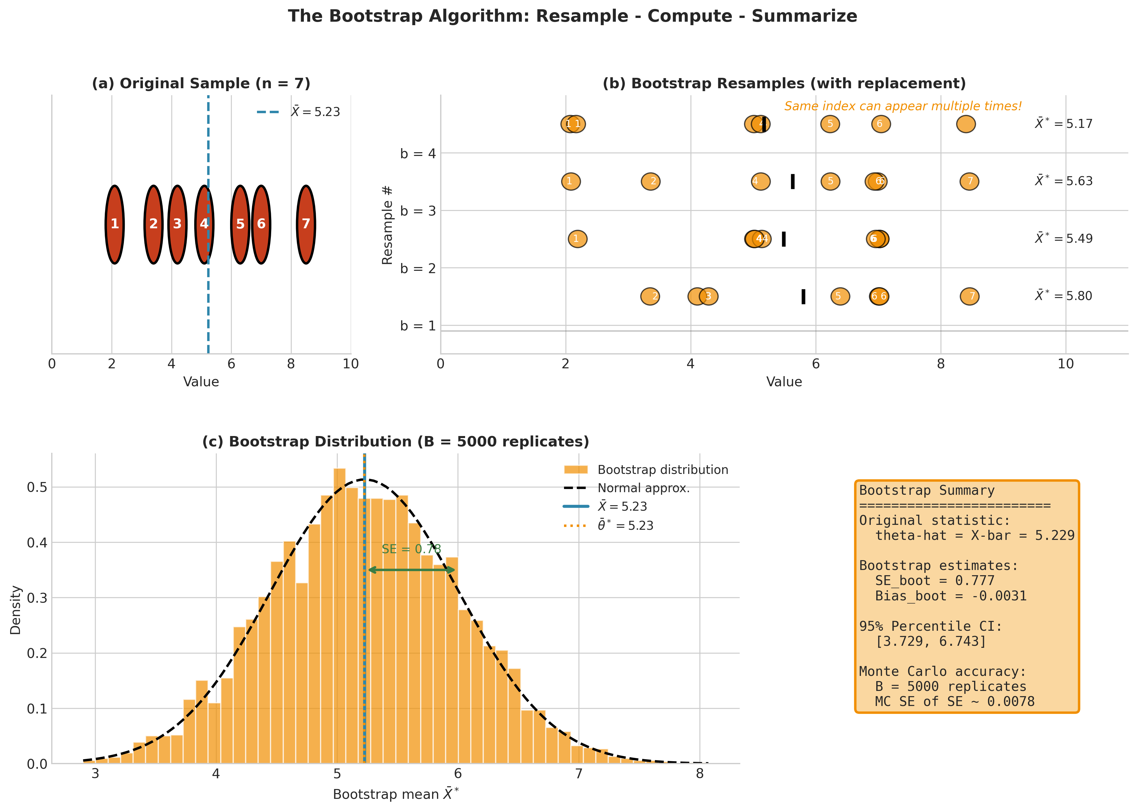
Fig. 143 Figure 4.3.1: The bootstrap algorithm in action. (a) Original sample with \(n = 7\) observations. (b) Four bootstrap resamples showing how the same index can appear multiple times. (c) The bootstrap distribution of \(\bar{X}^*\) from 5,000 replicates, with SE and CI summaries.

Properties of Bootstrap Samples

Understanding the structure of bootstrap samples provides insight into the method’s behavior.

Multinomial Structure: The resample counts \((N_1, \ldots, N_n)\), where \(N_i\) is the number of times observation \(i\) appears in a bootstrap sample, follow

\[(N_1, \ldots, N_n) \sim \text{Multinomial}\left(n; \frac{1}{n}, \ldots, \frac{1}{n}\right)\]

Each \(N_i\) has \(\mathbb{E}[N_i] = 1\) and \(\text{Var}(N_i) = (n-1)/n\). For large \(n\), \(N_i \approx \text{Poisson}(1)\).

Expected Unique Observations: The expected number of unique observations in a bootstrap sample is

\[\mathbb{E}[U] = n \cdot \left(1 - \left(1 - \frac{1}{n}\right)^n\right) \to n(1 - e^{-1}) \approx 0.632n\]

Thus, about 63.2% of observations appear at least once, while 36.8% are omitted (and some appear multiple times). This “leaving out” property is exploited later for the .632 estimator in prediction error estimation.

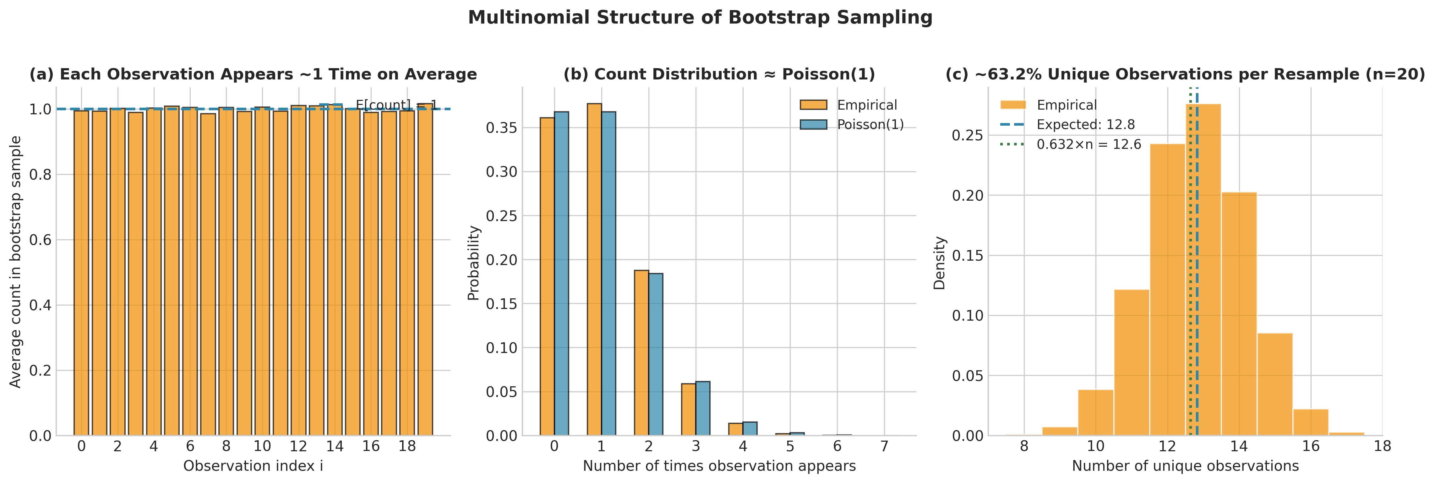
Fig. 144 Figure 4.3.2: Multinomial structure of bootstrap sampling. (a) Each observation appears on average once per resample. (b) Individual inclusion counts follow approximately Poisson(1). (c) About 63.2% of observations are unique in each bootstrap sample.

Python Implementation

import numpy as np

def bootstrap_distribution(data, statistic, B=5000, seed=None):
    """
    Generate the bootstrap distribution of a statistic.

    Parameters
    ----------
    data : array_like
        Original data (1D array for univariate, 2D with observations
        along first axis for multivariate).
    statistic : callable
        Function that computes the statistic from data.
    B : int
        Number of bootstrap replicates.
    seed : int, optional
        Random seed for reproducibility.

    Returns
    -------
    theta_star : ndarray
        Bootstrap distribution of the statistic.
    theta_hat : float or ndarray
        Original estimate from the data.
    """
    rng = np.random.default_rng(seed)
    data = np.asarray(data)
    n = len(data)  # observations along first axis

    # Compute original estimate (once!)
    theta_hat = statistic(data)

    # Pre-allocate based on statistic output shape
    theta_hat_arr = np.asarray(theta_hat)
    if theta_hat_arr.ndim == 0:
        theta_star = np.empty(B)
    else:
        theta_star = np.empty((B,) + theta_hat_arr.shape)

    for b in range(B):
        idx = rng.integers(0, n, size=n)  # sample with replacement
        theta_star[b] = statistic(data[idx])

    return theta_star, theta_hat

Bootstrap Standard Errors

The most fundamental bootstrap quantity is the standard error—the standard deviation of the sampling distribution. The bootstrap SE is simply the sample standard deviation of the bootstrap replicates.

Definition and Computation

For a statistic \(\hat{\theta} = T(X_{1:n})\) targeting \(\theta = T(F)\), the true standard error is \(\text{SE}(\hat{\theta}) = \sqrt{\text{Var}_F(\hat{\theta})}\). This measures the spread of \(\hat{\theta}\) over hypothetical repeated samples from \(F\).

The bootstrap standard error estimates this by:

(179)\[\widehat{\text{SE}}_{\text{boot}} = \sqrt{\frac{1}{B-1} \sum_{b=1}^{B} \left(\hat{\theta}^*_b - \bar{\theta}^*\right)^2}\]

where \(\bar{\theta}^* = \frac{1}{B}\sum_{b=1}^{B} \hat{\theta}^*_b\) is the mean of bootstrap replicates.

For vector statistics \(\hat{\boldsymbol{\theta}} \in \mathbb{R}^p\), the bootstrap covariance matrix is:

\[\widehat{\text{Cov}}_{\text{boot}}(\hat{\boldsymbol{\theta}}) = \frac{1}{B-1} \sum_{b=1}^{B} (\hat{\boldsymbol{\theta}}^*_b - \bar{\boldsymbol{\theta}}^*)(\hat{\boldsymbol{\theta}}^*_b - \bar{\boldsymbol{\theta}}^*)^\top\]

Marginal standard errors are the square roots of diagonal entries.

Choosing B: The Number of Bootstrap Replicates

The choice of \(B\) involves a tradeoff between computational cost and Monte Carlo accuracy. Two sources of uncertainty coexist:

1. Statistical uncertainty: The inherent variability of \(\hat{\theta}\) across samples from \(F\).

2. Monte Carlo error: Variability from using finite \(B\) instead of the full bootstrap distribution.

We want Monte Carlo error to be negligible relative to statistical uncertainty.

Monte Carlo error of the bootstrap SE: When \(\hat{\theta}^*\) is approximately normal with standard deviation \(\sigma\), the Monte Carlo standard deviation of \(\widehat{\text{SE}}_{\text{boot}}\) is approximately:

\[\text{sd}_{\text{MC}}\left(\widehat{\text{SE}}_{\text{boot}}\right) \approx \frac{\widehat{\text{SE}}_{\text{boot}}}{\sqrt{2(B-1)}}\]

Practical guidance:

• SE estimation only: \(B \approx 1{,}000\) to \(2{,}000\) usually suffices.

• Confidence intervals (which use tail quantiles): \(B \geq 5{,}000\), often \(10{,}000\).

• Stability check: Increase \(B\) in steps (e.g., \(1{,}000 \to 2{,}000 \to 5{,}000\)) and stop when \(\widehat{\text{SE}}_{\text{boot}}\) changes by less than your tolerance (e.g., \(< 1\%\)).

Monte Carlo error for CI endpoints: Tail quantiles are inherently noisier than central summaries like SE. The Monte Carlo error of the \(\alpha/2\) quantile scales as \(O(1/\sqrt{B})\) but also depends on the bootstrap density at that quantile. Endpoints stabilize more slowly than SE—rerunning with different seeds or using repeated bootstraps can assess this variability.

Comparison with Analytical Standard Errors

When analytical formulas exist, bootstrap SE should agree closely—this serves as a sanity check.

Mean: For \(\hat{\theta} = \bar{X}\), the analytical SE is \(s/\sqrt{n}\) where \(s\) is the sample standard deviation. Bootstrap SE should match this closely.

Median: The analytical SE involves the unknown density at the median: \(\text{SE}(\text{med}) \approx 1/(2f(m)\sqrt{n})\). Bootstrap SE sidesteps this estimation problem and adapts to skewness.

Correlation: Analytical SE for Pearson correlation \(r\) involves complex expressions. Bootstrap SE adapts to boundary effects; as \(|r| \to 1\), variability on the \(r\)-scale often shrinks, but the distribution becomes strongly skewed and non-normal, motivating transformations (Fisher \(z\)) or percentile-style intervals.

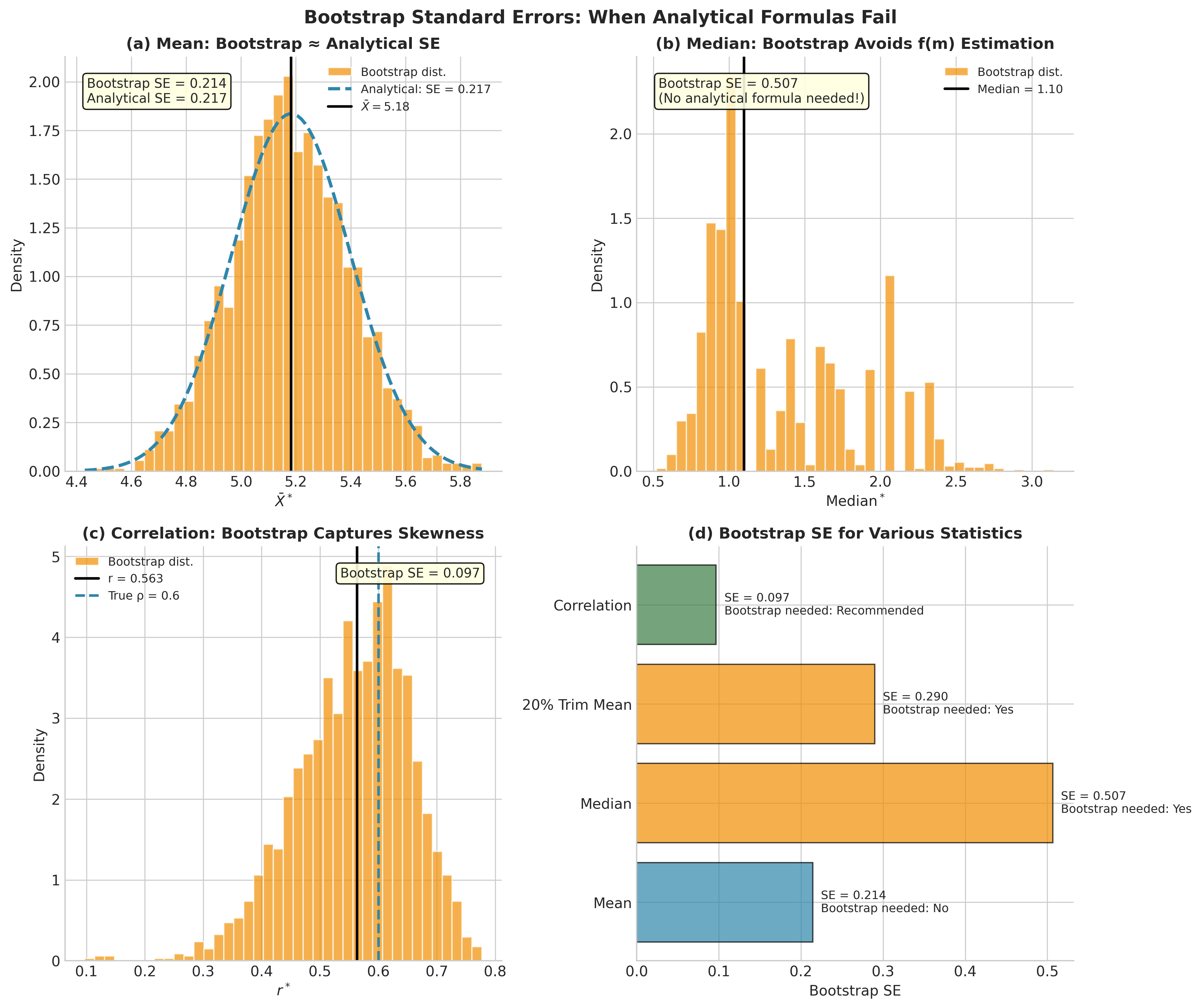
Fig. 145 Figure 4.3.3: Bootstrap SE compared to analytical formulas. (a) For the mean, bootstrap matches \(s/\sqrt{n}\) closely. (b) For the median, bootstrap avoids difficult density estimation. (c) For correlation, bootstrap captures the complex sampling behavior. (d) Summary showing when bootstrap is necessary.

Python Implementation

def bootstrap_se(data, statistic, B=2000, seed=None):
    """
    Compute bootstrap standard error for a statistic.

    Parameters
    ----------
    data : array_like
        Original data.
    statistic : callable
        Function that computes the statistic.
    B : int
        Number of bootstrap replicates.
    seed : int, optional
        Random seed.

    Returns
    -------
    se_boot : float
        Bootstrap standard error.
    theta_hat : float
        Original estimate.
    """
    theta_star, theta_hat = bootstrap_distribution(data, statistic, B, seed)
    se_boot = np.std(theta_star, ddof=1)
    return se_boot, theta_hat

Example 💡 Bootstrap SE for the Sample Median

Given: \(n = 60\) observations from a log-normal distribution (skewed data).

Find: Bootstrap SE for the sample median.

Python implementation:

import numpy as np

# Generate skewed data
rng = np.random.default_rng(42)
n = 60
x = np.exp(rng.normal(0, 1, size=n))  # log-normal

# Original median
median_hat = np.median(x)

# Bootstrap
B = 5000
median_star = np.empty(B)
for b in range(B):
    idx = rng.integers(0, n, size=n)
    median_star[b] = np.median(x[idx])

se_boot = np.std(median_star, ddof=1)

print(f"Sample median: {median_hat:.4f}")
print(f"Bootstrap SE:  {se_boot:.4f}")

Result: The bootstrap provides an SE estimate without requiring density estimation at the median. The histogram of median_star typically shows some skewness, reflecting the asymmetry of the underlying distribution.

Bootstrap Bias Estimation

Beyond standard errors, the bootstrap can estimate bias—the systematic difference between the expected value of an estimator and the true parameter.

Definition and Estimation

For a statistic \(\hat{\theta} = T(X_{1:n})\) targeting \(\theta = T(F)\), the finite-sample bias under \(F\) is:

\[\text{Bias}_F(\hat{\theta}) = \mathbb{E}_F[\hat{\theta}] - \theta\]

The bootstrap estimates this by replacing \(F\) with \(\hat{F}_n\):

(180)\[\widehat{\text{Bias}}_{\text{boot}} = \bar{\theta}^* - \hat{\theta}\]

where \(\bar{\theta}^* = \frac{1}{B}\sum_{b=1}^B \hat{\theta}^*_b\) approximates \(\mathbb{E}_{\hat{F}_n}[\hat{\theta}]\).

Bias-Corrected Estimator

If the bootstrap detects substantial bias, we can construct a bias-corrected estimator:

(181)\[\hat{\theta}^{bc} = \hat{\theta} - \widehat{\text{Bias}}_{\text{boot}} = 2\hat{\theta} - \bar{\theta}^*\]

If the bootstrap average \(\bar{\theta}^*\) overshoots \(\hat{\theta}\), we pull back; if it undershoots, we push up.

When to Apply Bias Correction

Bias correction is not always beneficial—it increases variance. The goal is to reduce mean squared error \(\text{MSE} = \text{Bias}^2 + \text{Var}\).

Rule of thumb: Compare \(|\widehat{\text{Bias}}_{\text{boot}}|\) to \(\widehat{\text{SE}}_{\text{boot}}\):

• If \(|\widehat{\text{Bias}}_{\text{boot}}| < 0.25 \cdot \widehat{\text{SE}}_{\text{boot}}\): Bias is negligible; correction rarely helps.

• If \(|\widehat{\text{Bias}}_{\text{boot}}| \approx 0.25\text{--}0.5 \cdot \widehat{\text{SE}}_{\text{boot}}\): Consider reporting both \(\hat{\theta}\) and \(\hat{\theta}^{bc}\).

• If \(|\widehat{\text{Bias}}_{\text{boot}}| > 0.5 \cdot \widehat{\text{SE}}_{\text{boot}}\): Bias correction may help, but check stability with larger \(B\).

Common Pitfall ⚠️

Variance inflation from bias correction: The corrected estimator \(\hat{\theta}^{bc}\) uses \(\bar{\theta}^*\), which has both Monte Carlo and statistical variability. This can make \(\hat{\theta}^{bc}\) noisier than \(\hat{\theta}\). Always report \(\widehat{\text{SE}}_{\text{boot}}\) alongside bias estimates, and increase \(B\) if conclusions depend on the correction.

Canonical Examples

Sample standard deviation: The sample SD with \(1/(n-1)\) divisor has small negative bias for estimating \(\sigma\). Bootstrap typically detects this, but correction is rarely needed.

Ratio estimators \(\hat{\theta} = \bar{X}/\bar{Y}\): Nonlinearity induces bias, especially when \(\bar{Y}\) is variable. Bootstrap bias can be non-negligible for small \(n\).

Log-scale back-transforms: If you estimate a mean on the log scale and exponentiate, Jensen’s inequality creates bias. Bootstrap can quantify (and sometimes correct) this.

Bootstrap Confidence Intervals

While standard errors summarize spread, confidence intervals provide ranges that capture the parameter with specified probability. The bootstrap offers several interval construction methods with different properties.

Percentile Interval

The simplest bootstrap interval uses the quantiles of the bootstrap distribution directly.

Definition: The \((1-\alpha)\) percentile interval is:

(182)\[\left[Q_{\alpha/2}(\hat{\theta}^*), Q_{1-\alpha/2}(\hat{\theta}^*)\right]\]

where \(Q_p(\hat{\theta}^*)\) denotes the \(p\)-th quantile of the bootstrap distribution.

Properties:

• Simple and automatic: No variance formula or studentization needed.

• Transformation invariant: If \(\phi(\cdot)\) is strictly monotone, the \(\phi\)-scale interval maps back exactly to the original scale.

• Respects skewness: Uses the shape of the bootstrap distribution directly.

Limitations:

• Coverage error can be non-negligible in small samples.

• Not centered at \(\hat{\theta}\); if the statistic is biased, the interval drifts.

• Can include impossible values near boundaries without truncation.

Basic (Pivotal) Interval

The basic interval (also called pivotal) reflects the percentile interval about \(\hat{\theta}\), partially correcting for bias drift.

Definition: The \((1-\alpha)\) basic interval is:

(183)\[\left[2\hat{\theta} - Q_{1-\alpha/2}(\hat{\theta}^*), 2\hat{\theta} - Q_{\alpha/2}(\hat{\theta}^*)\right]\]

Derivation: The bootstrap distribution of \(\hat{\theta}^* - \hat{\theta}\) approximates the distribution of \(\hat{\theta} - \theta\). Inverting this relationship gives the basic interval.

Properties:

• Centered at \(\hat{\theta}\), which partially corrects bias drift seen in percentile intervals.

• Not transformation invariant.

• Still sensitive to skewness.

Normal Approximation Interval

When the bootstrap distribution is approximately normal, we can use:

\[\hat{\theta} \pm z_{1-\alpha/2} \cdot \widehat{\text{SE}}_{\text{boot}}\]

where \(z_{1-\alpha/2}\) is the standard normal quantile.

This is appropriate when the bootstrap histogram looks symmetric and bell-shaped, but ignores any asymmetry in the true sampling distribution.

Comparison of Interval Methods

Table 44 Bootstrap Confidence Interval Methods

Method	Formula	Strengths	Limitations
Percentile	\([Q_{\alpha/2}, Q_{1-\alpha/2}]\)	Simple; transformation invariant; captures skewness	Can drift with bias; boundary issues
Basic	\([2\hat{\theta} - Q_{1-\alpha/2}, 2\hat{\theta} - Q_{\alpha/2}]\)	Corrects bias drift; simple	Not transformation invariant; skewness sensitive
Normal	\(\hat{\theta} \pm z \cdot \widehat{\text{SE}}_{\text{boot}}\)	Fast; symmetric	Ignores skewness; poor for non-normal cases

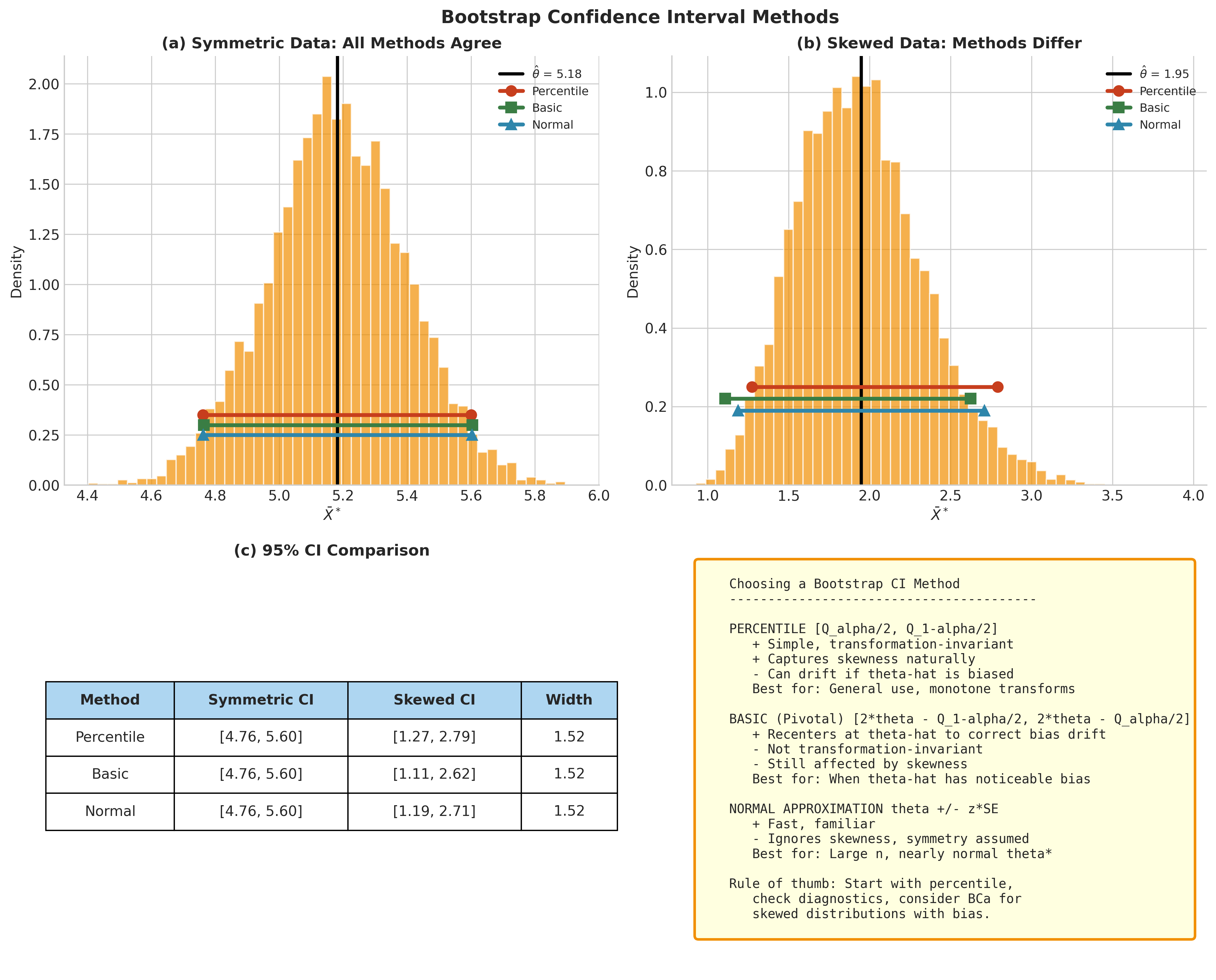
Fig. 146 Figure 4.3.4: Bootstrap CI methods compared. (a) For symmetric data, all three methods (percentile, basic, normal) give similar intervals. (b) For skewed data, the methods diverge—percentile captures asymmetry while normal assumes symmetry. (c-d) Practical recommendations for choosing among methods.

Python Implementation

def bootstrap_ci(data, statistic, alpha=0.05, B=10000,
                 method='percentile', seed=None):
    """
    Compute bootstrap confidence interval.

    Parameters
    ----------
    data : array_like
        Original data.
    statistic : callable
        Function that computes the statistic.
    alpha : float
        Significance level (1-alpha confidence).
    B : int
        Number of bootstrap replicates.
    method : str
        'percentile', 'basic', or 'normal'.
    seed : int, optional
        Random seed.

    Returns
    -------
    ci : tuple
        (lower, upper) confidence bounds.
    theta_hat : float
        Original estimate.
    """
    theta_star, theta_hat = bootstrap_distribution(data, statistic, B, seed)

    if method == 'percentile':
        lower = np.quantile(theta_star, alpha/2)
        upper = np.quantile(theta_star, 1 - alpha/2)

    elif method == 'basic':
        q_lower = np.quantile(theta_star, alpha/2)
        q_upper = np.quantile(theta_star, 1 - alpha/2)
        lower = 2*theta_hat - q_upper
        upper = 2*theta_hat - q_lower

    elif method == 'normal':
        se_boot = np.std(theta_star, ddof=1)
        from scipy import stats
        z = stats.norm.ppf(1 - alpha/2)
        lower = theta_hat - z * se_boot
        upper = theta_hat + z * se_boot

    else:
        raise ValueError(f"Unknown method: {method}")

    return (lower, upper), theta_hat

Example 💡 Comparing Interval Methods for the Correlation Coefficient

Given: \(n = 100\) bivariate observations with true correlation \(\rho = 0.6\).

Find: 95% bootstrap CIs using percentile, basic, and normal methods.

Python implementation:

import numpy as np
from scipy import stats

# Generate correlated data
rng = np.random.default_rng(123)
n = 100
rho = 0.6
cov = np.array([[1, rho], [rho, 1]])
xy = rng.multivariate_normal([0, 0], cov, size=n)

def correlation(data):
    return np.corrcoef(data[:, 0], data[:, 1])[0, 1]

r_hat = correlation(xy)
print(f"Sample correlation: {r_hat:.4f}")

# Bootstrap
B = 10000
r_star = np.empty(B)
for b in range(B):
    idx = rng.integers(0, n, size=n)
    r_star[b] = correlation(xy[idx])

# Percentile CI
ci_perc = np.quantile(r_star, [0.025, 0.975])

# Basic CI
q_lo, q_hi = np.quantile(r_star, [0.025, 0.975])
ci_basic = (2*r_hat - q_hi, 2*r_hat - q_lo)

# Normal CI
se_boot = np.std(r_star, ddof=1)
z = stats.norm.ppf(0.975)
ci_normal = (r_hat - z*se_boot, r_hat + z*se_boot)

print(f"Percentile CI: [{ci_perc[0]:.4f}, {ci_perc[1]:.4f}]")
print(f"Basic CI:      [{ci_basic[0]:.4f}, {ci_basic[1]:.4f}]")
print(f"Normal CI:     [{ci_normal[0]:.4f}, {ci_normal[1]:.4f}]")

Result: For correlation away from boundaries (\(\pm 1\)), the three methods typically agree closely. Near boundaries, the bootstrap distribution becomes skewed, and percentile/basic intervals may differ from normal intervals.

Bootstrap for Regression

Regression models require careful attention to what gets resampled. The appropriate scheme depends on whether the regressors are treated as fixed (controlled by design) or random (observed from a population), and whether errors are homoscedastic or heteroscedastic.

This section develops three resampling schemes: residual bootstrap (fixed-X, homoscedastic), pairs bootstrap (random-X or heteroscedastic), and wild bootstrap (fixed-X, heteroscedastic). Understanding when to use each connects bootstrap methodology to experimental design principles.

The Regression Setup

Consider the linear model:

\[Y_i = \mathbf{x}_i^\top \boldsymbol{\beta} + \varepsilon_i, \quad i = 1, \ldots, n\]

or in matrix form:

\[\mathbf{Y} = \mathbf{X}\boldsymbol{\beta} + \boldsymbol{\varepsilon}\]

where \(\mathbf{X} \in \mathbb{R}^{n \times p}\) is the design matrix (including intercept), \(\boldsymbol{\beta} \in \mathbb{R}^p\) are coefficients, and \(\boldsymbol{\varepsilon}\) are errors.

The OLS estimator is \(\hat{\boldsymbol{\beta}} = (\mathbf{X}^\top\mathbf{X})^{-1}\mathbf{X}^\top\mathbf{Y}\).

Under the classical model with \(\mathbb{E}[\boldsymbol{\varepsilon}|\mathbf{X}] = \mathbf{0}\) and \(\text{Var}(\boldsymbol{\varepsilon}|\mathbf{X}) = \sigma^2\mathbf{I}_n\):

\[\text{Var}(\hat{\boldsymbol{\beta}}|\mathbf{X}) = \sigma^2(\mathbf{X}^\top\mathbf{X})^{-1}\]

But what if assumptions fail? What if \(n\) is modest? What if the statistic of interest is a complex function of \(\hat{\boldsymbol{\beta}}\)? Bootstrap provides a flexible alternative.

Residual Bootstrap (Fixed-X, Homoscedastic)

When the design is fixed (as in designed experiments) and errors are exchangeable (homoscedastic), we resample residuals while keeping \(\mathbf{X}\) fixed.

Algorithm: Residual Bootstrap

Input: Design matrix X, response Y, number of replicates B
Output: Bootstrap distribution of β̂*

1. Fit OLS: β̂ = (X'X)⁻¹X'Y
2. Compute fitted values: Ŷ = Xβ̂
3. Compute residuals: ê = Y - Ŷ
4. Center residuals: ẽᵢ = êᵢ - mean(ê)  [ensures Σẽᵢ = 0]
   (With an intercept in the model, Σêᵢ = 0 up to numerical error;
    centering is still good practice and matters in models without intercept)
5. For b = 1, ..., B:
   a. Sample ẽ*₁, ..., ẽ*ₙ with replacement from {ẽ₁, ..., ẽₙ}
   b. Create: Y*ᵢ = Ŷᵢ + ẽ*ᵢ for all i
   c. Refit: β̂*_b = (X'X)⁻¹X'Y*
6. Return {β̂*₁, ..., β̂*_B}

When to use: Designed experiments (DOE) where regressors are set by the experimenter. The fixed-X perspective is appropriate when \(\mathbf{X}\) is under experimental control, not sampled from a population.

Assumptions: Errors are iid (or at least exchangeable) and homoscedastic. The residual bootstrap fails under heteroscedasticity because resampling mixes residuals from low-variance and high-variance regions.

Leverage-Adjusted Residual Bootstrap

High-leverage observations have residuals that are systematically smaller in magnitude (they “pull” the fit toward themselves). For better finite-sample behavior, we can adjust for leverage.

The leverage of observation \(i\) is \(h_{ii}\), the \(i\)-th diagonal of the hat matrix \(\mathbf{H} = \mathbf{X}(\mathbf{X}^\top\mathbf{X})^{-1}\mathbf{X}^\top\).

Algorithm modification:

1. Compute studentized residuals: \(r_i = \hat{e}_i / \sqrt{1 - h_{ii}}\)

2. Center: \(\tilde{r}_i = r_i - \bar{r}\)

3. Resample \(\tilde{r}^*\) and set \(\tilde{e}^*_i = \tilde{r}^*_i \sqrt{1 - h_{ii}}\)

4. Continue as before with \(Y^*_i = \hat{Y}_i + \tilde{e}^*_i\)

This improves calibration when leverage varies substantially across observations.

Pairs Bootstrap (Random-X)

When observations \((\mathbf{x}_i, Y_i)\) are iid draws from a joint distribution—as in observational studies—we resample entire rows (cases).

Algorithm: Pairs (Case) Bootstrap

Input: Data matrix (X, Y) with n rows, number of replicates B
Output: Bootstrap distribution of β̂*

1. Fit OLS on original data: β̂
2. For b = 1, ..., B:
   a. Sample indices I₁, ..., Iₙ with replacement from {1, ..., n}
   b. Form bootstrap dataset: (X*, Y*) = rows {I₁, ..., Iₙ}
   c. Refit: β̂*_b = (X*'X*)⁻¹X*'Y*
3. Return {β̂*₁, ..., β̂*_B}

When to use: Observational studies where both \(X\) and \(Y\) are measured (not controlled). Also use when heteroscedasticity is present and you want robustness without modeling the variance structure.

Properties:

• Automatically respects heteroscedasticity tied to \(X\)

• Preserves the joint distribution of \((X, Y)\)

• More variable than residual bootstrap when leverage points are rare (some resamples may omit them)

• Robust to model misspecification

Connection to design: Pairs resampling treats the entire observation \((\mathbf{x}_i, Y_i)\) as the sampling unit, appropriate when data come from random sampling rather than controlled experimentation.

Wild Bootstrap (Fixed-X, Heteroscedastic)

When the design is fixed but errors are heteroscedastic, the wild bootstrap preserves the \(\mathbf{X}\) structure while respecting location-specific variance.

Algorithm: Wild Bootstrap (Rademacher)

Input: Design matrix X, response Y, number of replicates B
Output: Bootstrap distribution of β̂*

1. Fit OLS: β̂, compute Ŷ and ê
2. For b = 1, ..., B:
   a. Generate w₁, ..., wₙ iid with P(wᵢ = ±1) = 1/2
   b. Create: Y*ᵢ = Ŷᵢ + wᵢ · êᵢ
   c. Refit: β̂*_b = (X'X)⁻¹X'Y*
3. Return {β̂*₁, ..., β̂*_B}

Weight choices: The multipliers \(w_i\) should satisfy \(\mathbb{E}[w_i] = 0\) and \(\mathbb{E}[w_i^2] = 1\).

• Rademacher: \(P(w_i = \pm 1) = 1/2\). Simple; preserves residual magnitude.

• Mammen: \(w_i \in \{-(√5-1)/2, (√5+1)/2\}\) with appropriate probabilities. Matches third moment of residuals.

Why it works: Multiplying residuals by \(\pm 1\) preserves mean zero and variance \(\hat{e}_i^2\), allowing heteroscedastic variance patterns to be respected. The fixed \(\mathbf{X}\) structure is maintained exactly.

Leverage Adjustment for Wild Bootstrap

For designs with high leverage points, finite-sample calibration improves when using HC2/HC3-scaled residuals before applying multipliers:

\[\tilde{e}_i = \frac{\hat{e}_i}{\sqrt{1 - h_{ii}}} \quad \text{(HC2-style)}\]

Then create \(Y^*_i = \hat{Y}_i + w_i \cdot \tilde{e}_i \cdot \sqrt{1 - h_{ii}}\) to map back to the original scale. This adjustment is especially important when leverage values \(h_{ii}\) vary substantially across observations.

Comparison of Regression Bootstrap Schemes

Table 45 Regression Bootstrap Scheme Selection

Aspect	Residual	Residual + Leverage	Pairs	Wild	Parametric
X treatment	Fixed	Fixed	Random	Fixed	Fixed
Homoscedasticity	Required	Required	Not required	Not required	Model-dependent
Heteroscedasticity	✗ Fails	✗ Fails	✓ Robust	✓ Handles	Model-dependent
Model misspecification	✗ Sensitive	✗ Sensitive	✓ Robust	✗ Sensitive	✗ Sensitive
DOE appropriate	✓ Yes	✓ Yes	✗ No	✓ Yes	✓ Yes
Observational appropriate	✗ No	✗ No	✓ Yes	Depends	Depends
Efficiency	High	High	Lower	Medium	Highest if correct

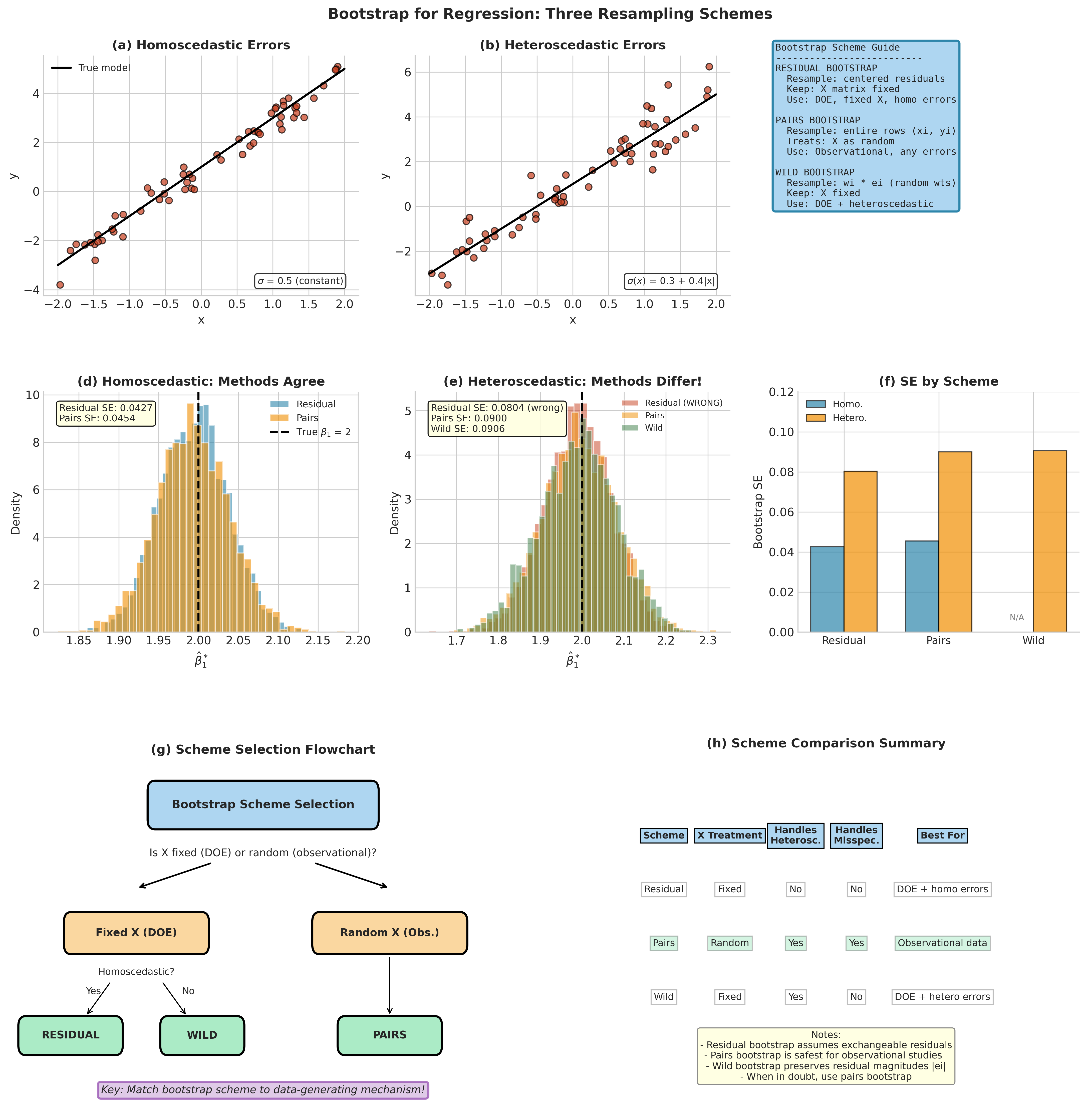
Fig. 147 Figure 4.3.5: Bootstrap schemes for regression. (a) Homoscedastic errors: variance is constant. (b) Heteroscedastic errors: variance depends on \(x\). (c) Scheme selection guide. (d) Under homoscedasticity, residual and pairs give similar results. (e) Under heteroscedasticity, residual bootstrap fails—pairs and wild are correct. (f) SE comparison across schemes.

Connection to Experimental Design

The choice between residual and pairs bootstrap connects deeply to the philosophy of experimental design:

Fixed-X (DOE perspective): In a designed experiment, the experimenter controls \(\mathbf{X}\). The randomness comes only from \(\varepsilon\). Residual bootstrap (or wild, for heteroscedasticity) respects this: it fixes \(\mathbf{X}\) and resamples only the error distribution.

Random-X (observational study perspective): In an observational study, both \(\mathbf{X}\) and \(Y\) are sampled. The joint distribution \(F_{X,Y}\) is the relevant population. Pairs bootstrap respects this: it resamples complete observations.

Practical guidance: Match your resampling scheme to the data-generating mechanism:

• Controlled experiment with treatment levels \(\to\) Residual (or Wild if heteroscedastic)

• Survey or observational sample \(\to\) Pairs

• Unknown or mixed \(\to\) Pairs (more robust, at some efficiency cost)

Scheme Selection Vignettes

Vignette 1: A chemist runs a DOE with 5 fixed temperature levels (20°, 40°, 60°, 80°, 100°C), measuring reaction yield at each. Residual plots show variance increasing with temperature.

Decision: Fixed X (DOE) + heteroscedastic errors → Wild bootstrap.

Vignette 2: An economist analyzes survey data on income vs. education, where both variables were recorded (not controlled) for a random sample of households.

Decision: Random X (observational) → Pairs bootstrap.

Vignette 3: A biologist studies plant growth under controlled light levels (fixed X), and residuals appear homoscedastic with no pattern in variance.

Decision: Fixed X (DOE) + homoscedastic errors → Residual bootstrap.

The key question is always: “What is the source of randomness in my data-generating process?”

Python Implementation for Regression Bootstrap

import numpy as np
from numpy.linalg import lstsq

def ols_fit(X, y):
    """Fit OLS, return coefficients."""
    return lstsq(X, y, rcond=None)[0]

def bootstrap_regression_residual(X, y, B=2000, seed=None):
    """
    Residual bootstrap for fixed-X homoscedastic regression.

    Parameters
    ----------
    X : ndarray, shape (n, p)
        Design matrix.
    y : ndarray, shape (n,)
        Response vector.
    B : int
        Number of bootstrap replicates.
    seed : int, optional
        Random seed.

    Returns
    -------
    beta_star : ndarray, shape (B, p)
        Bootstrap distribution of coefficient estimates.
    """
    rng = np.random.default_rng(seed)
    n, p = X.shape

    # Original fit
    beta_hat = ols_fit(X, y)
    y_hat = X @ beta_hat
    residuals = y - y_hat

    # Center residuals
    residuals_centered = residuals - residuals.mean()

    beta_star = np.empty((B, p))
    for b in range(B):
        # Resample residuals
        idx = rng.integers(0, n, size=n)
        e_star = residuals_centered[idx]
        y_star = y_hat + e_star
        beta_star[b] = ols_fit(X, y_star)

    return beta_star

def bootstrap_regression_pairs(X, y, B=2000, seed=None):
    """
    Pairs bootstrap for random-X or heteroscedastic regression.

    Parameters
    ----------
    X : ndarray, shape (n, p)
        Design matrix.
    y : ndarray, shape (n,)
        Response vector.
    B : int
        Number of bootstrap replicates.
    seed : int, optional
        Random seed.

    Returns
    -------
    beta_star : ndarray, shape (B, p)
        Bootstrap distribution of coefficient estimates.
    """
    rng = np.random.default_rng(seed)
    n, p = X.shape

    beta_star = np.empty((B, p))
    for b in range(B):
        # Resample rows (cases)
        idx = rng.integers(0, n, size=n)
        X_star = X[idx]
        y_star = y[idx]
        beta_star[b] = ols_fit(X_star, y_star)

    return beta_star

def bootstrap_regression_wild(X, y, B=2000, seed=None):
    """
    Wild bootstrap (Rademacher) for fixed-X heteroscedastic regression.

    Parameters
    ----------
    X : ndarray, shape (n, p)
        Design matrix.
    y : ndarray, shape (n,)
        Response vector.
    B : int
        Number of bootstrap replicates.
    seed : int, optional
        Random seed.

    Returns
    -------
    beta_star : ndarray, shape (B, p)
        Bootstrap distribution of coefficient estimates.
    """
    rng = np.random.default_rng(seed)
    n, p = X.shape

    # Original fit
    beta_hat = ols_fit(X, y)
    y_hat = X @ beta_hat
    residuals = y - y_hat

    beta_star = np.empty((B, p))
    for b in range(B):
        # Rademacher weights
        w = rng.choice([-1.0, 1.0], size=n)
        e_star = w * residuals
        y_star = y_hat + e_star
        beta_star[b] = ols_fit(X, y_star)

    return beta_star

Example 💡 Comparing Bootstrap Schemes Under Heteroscedasticity

Given: Regression data with heteroscedastic errors (variance increases with \(|x|\)).

Find: Compare SE estimates from residual, pairs, and wild bootstrap.

Python implementation:

import numpy as np

# Generate heteroscedastic data
rng = np.random.default_rng(42)
n = 150
x = rng.uniform(-2, 2, size=n)
sigma_i = 0.3 + 0.7 * np.abs(x)  # Heteroscedastic: variance depends on |x|
eps = rng.normal(0, sigma_i)
y = 1 + 2*x + eps

# Design matrix
X = np.column_stack([np.ones(n), x])

# Classical OLS SE (assumes homoscedasticity)
beta_hat = np.linalg.lstsq(X, y, rcond=None)[0]
y_hat = X @ beta_hat
residuals = y - y_hat
sigma2_hat = np.sum(residuals**2) / (n - 2)
XtX_inv = np.linalg.inv(X.T @ X)
se_classical = np.sqrt(sigma2_hat * np.diag(XtX_inv))

# Bootstrap SEs
B = 5000
beta_residual = bootstrap_regression_residual(X, y, B, seed=1)
beta_pairs = bootstrap_regression_pairs(X, y, B, seed=2)
beta_wild = bootstrap_regression_wild(X, y, B, seed=3)

print("SE estimates for slope coefficient:")
print(f"  Classical (wrong):     {se_classical[1]:.4f}")
print(f"  Residual bootstrap:    {beta_residual[:, 1].std():.4f}")
print(f"  Pairs bootstrap:       {beta_pairs[:, 1].std():.4f}")
print(f"  Wild bootstrap:        {beta_wild[:, 1].std():.4f}")

Result: Under heteroscedasticity, classical SE and residual bootstrap underestimate uncertainty because they assume constant variance. Pairs and wild bootstrap give more accurate (larger) SE estimates that properly reflect the heterogeneous variability.

Bootstrap Diagnostics

The bootstrap produces more than a number—the collection \(\{\hat{\theta}^*_b\}_{b=1}^B\) contains shape, skewness, and stability information that should guide interval choice and identify potential problems.

Core Diagnostic Displays

Always produce these visualizations when using bootstrap methods:

1. Histogram/density of \(\hat{\theta}^*\): Look for symmetry, skewness, heavy tails, multimodality.

2. Overlay of \(\hat{\theta}\) and CI endpoints: Visual check that the interval makes sense.

3. Normal Q-Q plot of \(\hat{\theta}^*\): Rough normality assessment; departures suggest percentile or BCa intervals may be preferable to normal approximation.

4. Endpoint stability plot: Track CI endpoints as \(B\) increases to verify Monte Carlo convergence.

Quantitative Shape Summaries

• Skewness: \(\gamma_1 = \mathbb{E}[(\hat{\theta}^* - \bar{\theta}^*)^3]/\text{SD}(\hat{\theta}^*)^3\). Large \(|\gamma_1|\) suggests percentile intervals may under-cover on the short tail.

• Kurtosis: Heavy tails inflate this; consider robust statistics or increased \(B\).

• Bias ratio: \(|\widehat{\text{Bias}}_{\text{boot}}| / \widehat{\text{SE}}_{\text{boot}}\). Values above 0.25 warrant attention; above 0.5 suggest BCa or reporting both corrected and uncorrected estimates.

Red Flags and Remedies

Table 46 Bootstrap Diagnostic Red Flags

Diagnostic finding	Suggested remedy
Strong skewness in \(\hat{\theta}^*\)	Use BCa or studentized bootstrap; avoid symmetric normal approximation
Heavy tails or multimodality	Consider robust statistics; increase \(B\); report multiple intervals
Many \(\hat{\theta}^*\) equal to \(\hat{\theta}\) (discreteness)	Use smoothed bootstrap for quantiles; parametric bootstrap if model is credible
Endpoints pile at bounds (e.g., CI crosses 0 for variances)	Use transformations (log-scale); parametric tails; truncate with caution
Large \(|\widehat{\text{Bias}}|\) relative to \(\widehat{\text{SE}}\)	Use BCa; report both \(\hat{\theta}\) and \(\hat{\theta}^{bc}\)
CI endpoints unstable as \(B\) increases	Increase \(B\); if persistent, statistic may be near-boundary or ill-posed

Interval Choice Decision Aid

Based on diagnostics, choose among interval methods:

1. \(\hat{\theta}^*\) roughly normal with small bias \(\to\) Normal approximation or basic interval; percentile also fine.

2. Skewed \(\hat{\theta}^*\) with modest bias \(\to\) Percentile or BCa (covered in Section 4.7).

3. Skewed with noticeable curvature \(\to\) BCa (requires acceleration constant from jackknife).

4. Extreme or boundary-driven target (max, outer quantiles) \(\to\) Parametric bootstrap, m-out-of-n, or EVT-based methods.

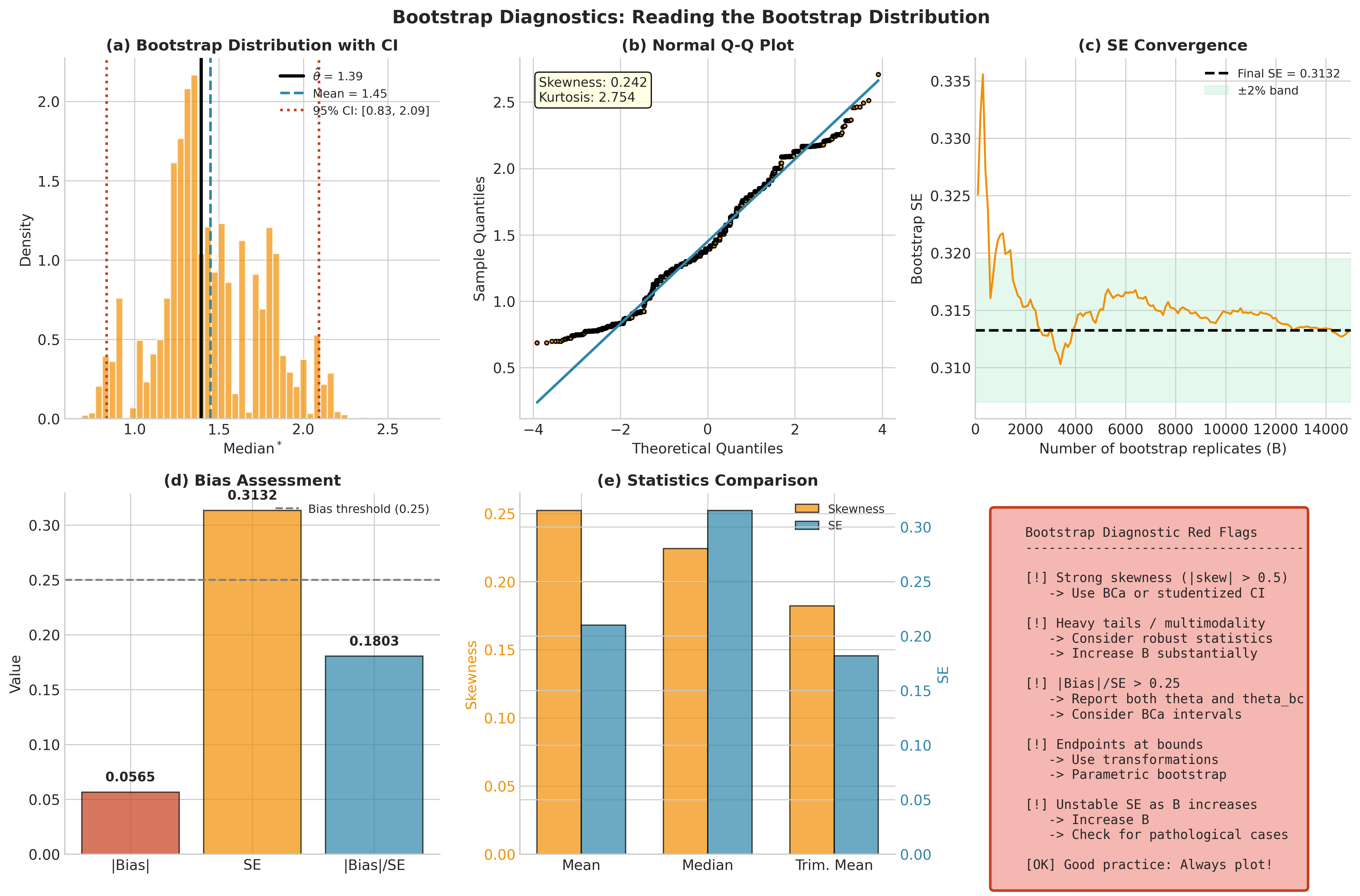
Fig. 148 Figure 4.3.6: Essential bootstrap diagnostics. (a) Histogram with CI endpoints marked. (b) Normal Q-Q plot revealing departures from normality. (c) SE convergence as \(B\) increases—use this to verify stability. (d) Bias assessment relative to SE. (e) Comparison across statistics. (f) Summary of red flags to watch for.

When Bootstrap Fails

The nonparametric bootstrap, while remarkably general, has known failure modes. Recognizing these prevents overconfidence in bootstrap results.

Extreme Value Statistics

Statistics like the sample maximum, minimum, range, and outer quantiles (1st, 99th percentile) suffer from support truncation: the bootstrap cannot generate values beyond the observed sample range.

Why it fails: The maximum of \(n\) bootstrap observations cannot exceed \(\max(X_1, \ldots, X_n)\). But the true sampling distribution of the maximum extends beyond observed data.

Remedies: - Parametric bootstrap with a fitted tail model (GPD, GEV from extreme value theory) - m-out-of-n bootstrap (subsample with \(m < n\)) - Bias-corrected endpoint estimators

Non-smooth and Non-regular Statistics

The bootstrap’s behavior depends critically on the regularity of the target functional.

Regular quantiles (e.g., median, quartiles): When the population density \(f(\xi_p) > 0\) at the \(p\)-th quantile, the bootstrap typically performs well. The variance is \(O(1/n)\) and standard theory applies.

Extreme quantiles and boundary cases: Outer quantiles (e.g., 1st or 99th percentile) suffer because the bootstrap cannot produce values beyond the observed sample range. As \(p \to 0\) or \(p \to 1\), bootstrap approximations degrade.

Genuinely non-smooth functionals (e.g., mode): The sample mode depends discontinuously on the data—small perturbations can cause large jumps. This violates the continuity conditions required for bootstrap consistency.

Why it fails: Bootstrap consistency typically requires Hadamard differentiability of the functional \(T\) at \(F\). The mode is the canonical example of a functional that fails this requirement. Quantiles with \(f(\xi_p) = 0\) or near zero also cause problems.

Remedies: - For extreme quantiles: parametric bootstrap or EVT-based methods - For mode: regularize (e.g., use highest-density region) or change the target - BCa intervals (partially correct for non-smoothness) - Smoothed bootstrap (add small noise before resampling) - Increase \(B\) substantially

Small Sample Sizes

With very small \(n\), bootstrap resamples don’t contain much new information—the bootstrap distribution is volatile and may poorly approximate the true sampling distribution.

Remedies: - Studentized (bootstrap-t) intervals - Parametric bootstrap if a credible model exists - Exact methods when available - Report wide intervals with appropriate caveats

Dependent Data

The iid bootstrap destroys dependence structure, leading to incorrect standard errors for time series, clustered, or spatial data.

Remedies (previewed for Section 4.9): - Block bootstrap (moving or circular blocks) - Stationary bootstrap (random block lengths) - Cluster bootstrap (resample clusters, not individuals) - Wild bootstrap with HAC-appropriate weights

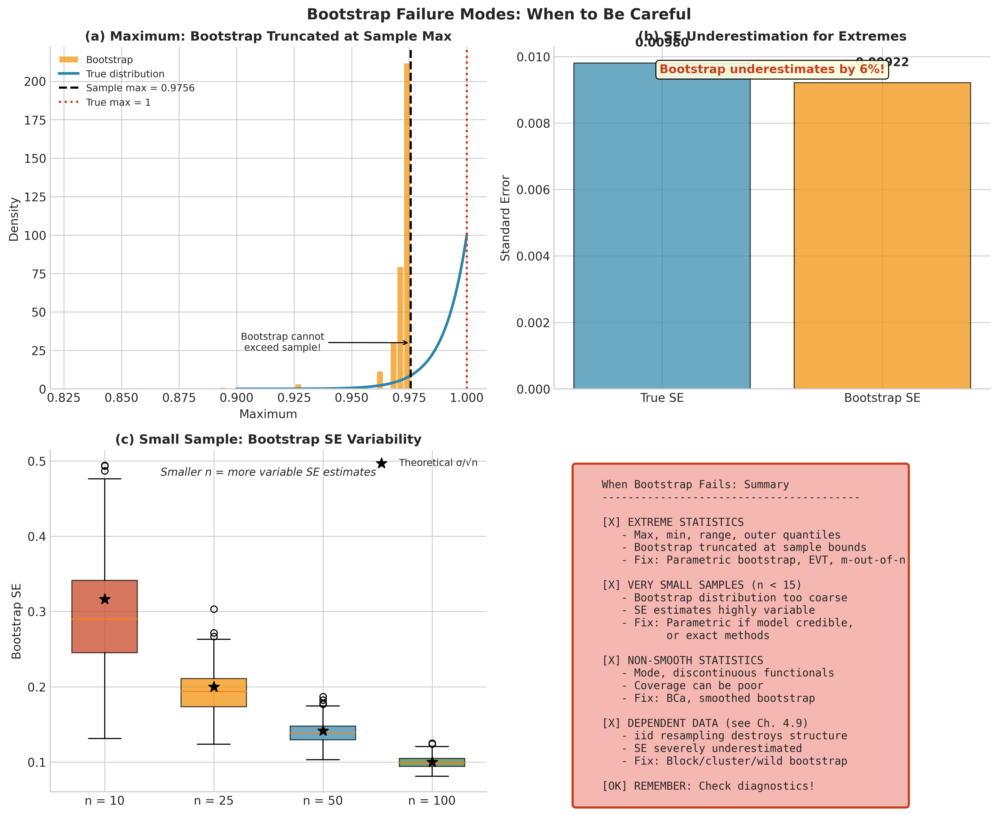
Fig. 149 Figure 4.3.7: When bootstrap fails. (a) For the sample maximum, bootstrap cannot exceed the observed range—it systematically underestimates tail behavior. (b) Comparison of true vs. bootstrap SE for extremes shows significant underestimation. (c) Small sample instability: SE estimates become highly variable as \(n\) decreases. (d) Summary of failure modes and remedies.

Practical Considerations

Numerical Stability and Precision

• Degenerate resamples: Some resamples may have identical observations (e.g., all bootstrap observations are the same point), making statistics like correlation or variance undefined.

  Explicit policy (choose one and be consistent):

  1. Skip and resample: If a replicate returns NaN/undefined, discard and draw again until \(B\) valid replicates are obtained.

  2. Record NaN and drop: Allow NaN values, then compute summaries (SE, quantiles) excluding them. Report the count of degenerate cases.

  3. Smoothed bootstrap: Add tiny jitter before resampling to prevent exact ties (see Section 4.7).

  For most applications, option 1 or 2 is appropriate. Always report if degeneracy occurred and how it was handled.

• Floating-point quantiles: Use consistent quantile interpolation methods (e.g., specify method in NumPy, type in R).

• Seed management: Always record seeds for reproducibility. For parallel execution, use independent RNG streams.

Computational Efficiency

• Vectorized index generation: Pre-generate an \(n \times B\) matrix of indices.

• Avoid redundant fitting: For regression, precompute \((\mathbf{X}^\top\mathbf{X})^{-1}\) when \(\mathbf{X}\) is fixed.

• Parallelization: Bootstrap replicates are independent—distribute across cores with proper seed management.

• Memory: Store only \(\hat{\theta}^*\), not full resampled datasets.

Reporting Standards

A bootstrap analysis should report:

1. The statistic \(T\) and its interpretation

2. The resampling scheme: iid observations, pairs, residual, wild

3. Number of replicates \(B\) and evidence of stability

4. RNG seed for reproducibility

5. Point estimate \(\hat{\theta}\) with \(\widehat{\text{SE}}_{\text{boot}}\)

6. Confidence interval with method (percentile, basic, BCa) and rationale

7. Diagnostics: histogram shape, bias assessment, any red flags

Bringing It All Together

The nonparametric bootstrap transforms the plug-in principle into a practical tool for inference. By replacing the unknown \(F\) with \(\hat{F}_n\) and simulating, we obtain standard errors, bias estimates, and confidence intervals for virtually any computable statistic.

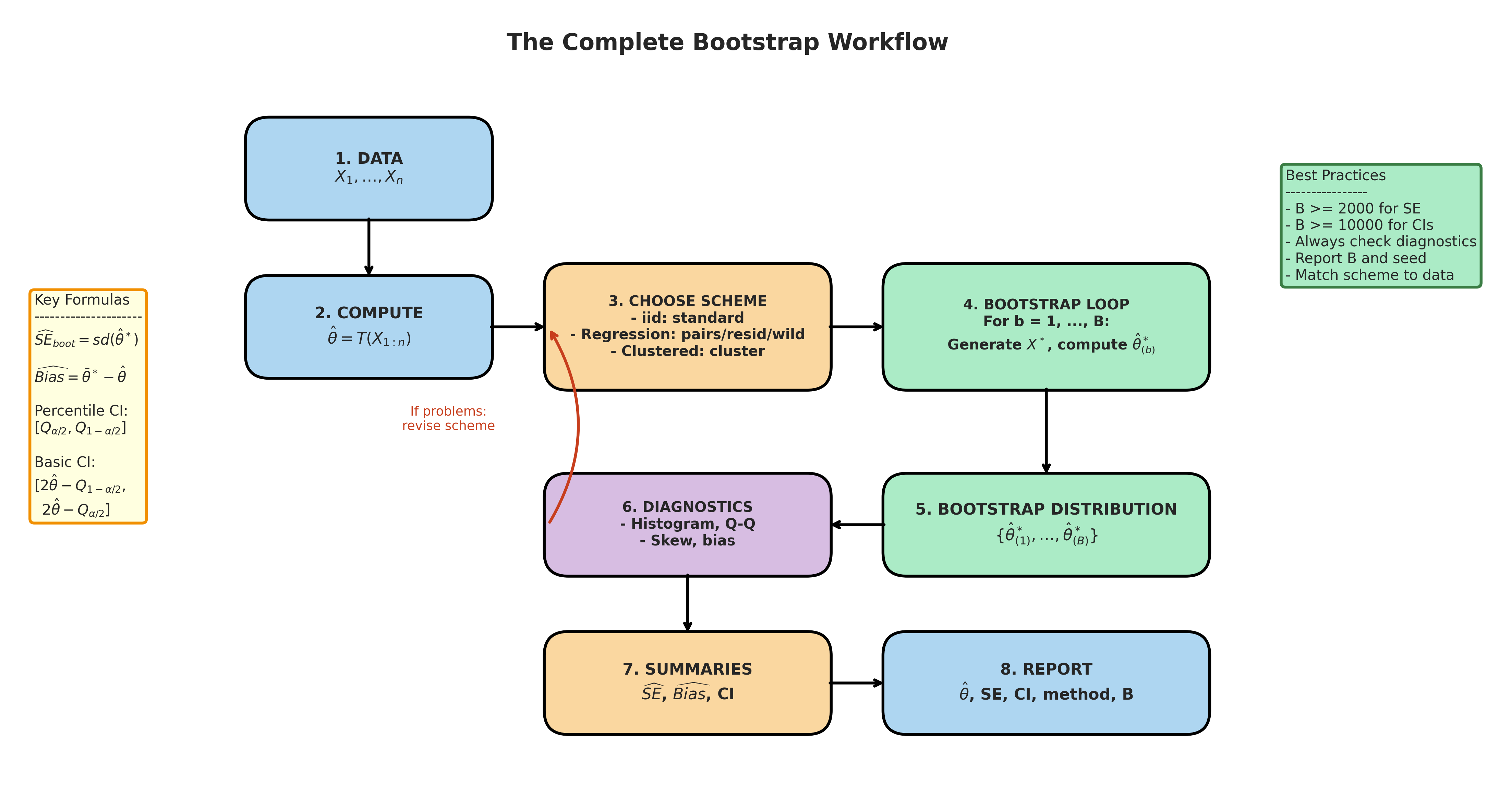
Fig. 150 Figure 4.3.8: The complete bootstrap workflow. Starting from data, we compute the statistic, choose an appropriate resampling scheme, run the bootstrap loop, build the bootstrap distribution, check diagnostics, extract summaries (SE, bias, CI), and report results with method details.

Summary of methods introduced:

• Bootstrap SE: Sample standard deviation of \(\{\hat{\theta}^*_b\}\)

• Bootstrap bias: \(\bar{\theta}^* - \hat{\theta}\)

• Percentile CI: Quantiles of bootstrap distribution

• Basic CI: Reflection of percentile about \(\hat{\theta}\)

• Residual bootstrap: Fixed-X, homoscedastic regression

• Pairs bootstrap: Random-X or robust to heteroscedasticity

• Wild bootstrap: Fixed-X with heteroscedasticity

Looking ahead: Section 4.4 develops the parametric bootstrap, which replaces \(\hat{F}_n\) with a fitted parametric model \(\hat{F}_{\hat{\theta}}\)—more efficient when the model is correct, but risky under misspecification. Section 4.5 introduces the jackknife, providing a different perspective on resampling that is particularly useful for bias correction and computing the acceleration constant in BCa intervals. Section 4.6 covers bootstrap hypothesis testing, including permutation tests. Section 4.7 develops advanced interval methods (BCa, studentized) with improved coverage properties.

Key Takeaways 📝

1. Core concept: The bootstrap approximates the sampling distribution by resampling from \(\hat{F}_n\)—computationally intensive but assumption-light

2. Computational insight: Bootstrap SE is simply \(\text{SD}(\hat{\theta}^*)\) over \(B\) replicates; choose \(B\) by stability (1,000–2,000 for SE, 5,000–10,000 for CIs)

3. Practical application: Match resampling scheme to data structure—residual for designed experiments with homoscedastic errors, pairs for observational studies, wild for heteroscedasticity with fixed design

4. Diagnostics are essential: Always examine the bootstrap distribution; shape guides interval choice and reveals failure modes

5. Outcome alignment: Develops simulation techniques for inference (LO 1), implements resampling for variability assessment and CIs (LO 3)

Exercises

Exercise 4.3.1: Bootstrap SE for the Mean

Background: The sample mean \(\bar{X}\) has analytical SE \(s/\sqrt{n}\), making it an ideal test case for bootstrap implementation.

Tasks:

1. Generate \(n = 50\) observations from \(N(0, 1)\). Compute the bootstrap SE for the mean using \(B = 2{,}000\) replicates. Compare to the analytical formula \(s/\sqrt{n}\).

2. Repeat with \(n = 50\) observations from \(\text{Exp}(1)\). How does the bootstrap SE compare to \(s/\sqrt{n}\)? Plot the histogram of \(\bar{X}^*\) and comment on its shape.

3. For the exponential case, how does the shape of the bootstrap distribution change as \(n\) increases to 200? Relate this to the Central Limit Theorem.

Hint: Use np.random.default_rng(seed) for reproducibility.

Solution

import numpy as np
import matplotlib.pyplot as plt

rng = np.random.default_rng(42)

# Part (a): Normal data
n, B = 50, 2000
x_norm = rng.normal(0, 1, size=n)

mean_hat = x_norm.mean()
se_analytical = x_norm.std(ddof=1) / np.sqrt(n)

mean_star = np.empty(B)
for b in range(B):
    idx = rng.integers(0, n, size=n)
    mean_star[b] = x_norm[idx].mean()

se_boot_norm = mean_star.std(ddof=1)
print(f"Normal data: Analytical SE = {se_analytical:.4f}, Bootstrap SE = {se_boot_norm:.4f}")
# Typical output: very close agreement

# Part (b): Exponential data
x_exp = rng.exponential(1.0, size=n)
se_analytical_exp = x_exp.std(ddof=1) / np.sqrt(n)

mean_star_exp = np.empty(B)
for b in range(B):
    idx = rng.integers(0, n, size=n)
    mean_star_exp[b] = x_exp[idx].mean()

se_boot_exp = mean_star_exp.std(ddof=1)
print(f"Exponential: Analytical SE = {se_analytical_exp:.4f}, Bootstrap SE = {se_boot_exp:.4f}")

# Histogram shows right skew for n=50
plt.hist(mean_star_exp, bins=40, edgecolor='black', alpha=0.7)
plt.axvline(x_exp.mean(), color='red', linestyle='--', label='Original mean')
plt.xlabel(r'$\bar{X}^*$')
plt.title('Bootstrap distribution of mean (Exponential, n=50)')
plt.legend()
plt.show()

# Part (c): CLT effect
n_large = 200
x_exp_large = rng.exponential(1.0, size=n_large)
mean_star_large = np.array([x_exp_large[rng.integers(0, n_large, size=n_large)].mean()
                             for _ in range(B)])
# Histogram is more symmetric with larger n

Key insights:

• For both distributions, bootstrap SE agrees closely with \(s/\sqrt{n}\) because the mean is a smooth, linear functional.

• The bootstrap histogram for exponential data shows right skew at \(n=50\), but becomes more symmetric as \(n\) increases per CLT.

• SE measures spread only; skewness affects interval choice but not SE validity.

Exercise 4.3.2: Bootstrap SE for the Median

Background: The median’s analytical SE involves the unknown density \(f\) at the median: \(\text{SE}(\text{med}) \approx 1/(2f(m)\sqrt{n})\). Bootstrap avoids this problem.

Tasks:

1. Generate \(n = 80\) observations from a log-normal distribution with \(\mu = 0, \sigma = 1\). Compute the bootstrap SE for the median using \(B = 5{,}000\).

2. Compare the bootstrap SEs for the mean, median, and 20% trimmed mean on the same data. Which has the smallest SE? Largest?

3. Add two outliers at \(+15\) and \(+20\) to your data. Recompute the three SEs. How do the relative SEs change?

4. What does this tell you about choosing between mean, median, and trimmed mean for skewed data with potential outliers?

Solution

import numpy as np
from scipy import stats

rng = np.random.default_rng(123)
n, B = 80, 5000

# Part (a): Log-normal data
x = np.exp(rng.normal(0, 1, size=n))

def bootstrap_se(data, statistic, B, rng):
    n = len(data)
    theta_star = np.empty(B)
    for b in range(B):
        idx = rng.integers(0, n, size=n)
        theta_star[b] = statistic(data[idx])
    return theta_star.std(ddof=1)

se_median = bootstrap_se(x, np.median, B, rng)
print(f"Median SE: {se_median:.4f}")

# Part (b): Compare three estimators
def trimmed_mean(z, prop=0.2):
    return stats.trim_mean(z, prop)

se_mean = bootstrap_se(x, np.mean, B, rng)
se_trim = bootstrap_se(x, lambda z: trimmed_mean(z, 0.2), B, rng)

print(f"Mean SE: {se_mean:.4f}")
print(f"Trimmed mean SE: {se_trim:.4f}")
print(f"Median SE: {se_median:.4f}")
# Typical: Mean > Trimmed > Median for right-skewed data

# Part (c): Add outliers
x_outliers = np.concatenate([x, [15.0, 20.0]])

se_mean_out = bootstrap_se(x_outliers, np.mean, B, rng)
se_trim_out = bootstrap_se(x_outliers, lambda z: trimmed_mean(z, 0.2), B, rng)
se_median_out = bootstrap_se(x_outliers, np.median, B, rng)

print(f"\nWith outliers:")
print(f"Mean SE: {se_mean_out:.4f} (increased significantly)")
print(f"Trimmed mean SE: {se_trim_out:.4f} (moderate increase)")
print(f"Median SE: {se_median_out:.4f} (minimal change)")

Key insights:

• For right-skewed data, the mean typically has the largest SE because it’s pulled by tail observations.

• Outliers dramatically increase mean SE but barely affect median SE.

• Trimmed mean provides a middle ground: robust to outliers while using more data than the median.

• Choice of estimator can matter more than choice of inference method.

Exercise 4.3.3: Bootstrap Bias Estimation

Background: The sample variance \(s^2 = \frac{1}{n-1}\sum(X_i - \bar{X})^2\) is unbiased for \(\sigma^2\), but the sample standard deviation \(s\) has a small negative bias for \(\sigma\).

Tasks:

1. Generate \(n = 30\) observations from \(N(0, 4)\) (so \(\sigma = 2\)). Compute the bootstrap estimate of bias for \(s\) using \(B = 5{,}000\).

2. Compute the bias-corrected estimator \(s^{bc} = 2s - \bar{s}^*\). Is it closer to the true \(\sigma = 2\)?

3. Compare \(|\widehat{\text{Bias}}|\) to \(\widehat{\text{SE}}_{\text{boot}}\). Based on the rule of thumb, should you apply bias correction?

4. Repeat parts (a)-(c) with \(n = 100\). How does the bias-to-SE ratio change?

Solution

import numpy as np

rng = np.random.default_rng(456)
sigma_true = 2.0
B = 5000

# Part (a) and (b): n = 30
n = 30
# Note: scale parameter is σ (std), not σ² (variance)
x = rng.normal(0, sigma_true, size=n)

s_hat = x.std(ddof=1)

s_star = np.empty(B)
for b in range(B):
    idx = rng.integers(0, n, size=n)
    s_star[b] = x[idx].std(ddof=1)

s_bar_star = s_star.mean()
se_boot = s_star.std(ddof=1)
bias_hat = s_bar_star - s_hat
s_bc = 2*s_hat - s_bar_star

print(f"n = {n}:")
print(f"  True σ = {sigma_true:.4f}")
print(f"  Sample s = {s_hat:.4f}")
print(f"  Bootstrap mean s̄* = {s_bar_star:.4f}")
print(f"  Estimated bias = {bias_hat:.4f}")
print(f"  Bias-corrected s_bc = {s_bc:.4f}")
print(f"  Bootstrap SE = {se_boot:.4f}")
print(f"  |Bias|/SE ratio = {abs(bias_hat)/se_boot:.4f}")

# Part (d): n = 100
n_large = 100
x_large = rng.normal(0, sigma_true, size=n_large)
s_hat_large = x_large.std(ddof=1)

s_star_large = np.array([x_large[rng.integers(0, n_large, size=n_large)].std(ddof=1)
                         for _ in range(B)])

bias_hat_large = s_star_large.mean() - s_hat_large
se_boot_large = s_star_large.std(ddof=1)

print(f"\nn = {n_large}:")
print(f"  |Bias|/SE ratio = {abs(bias_hat_large)/se_boot_large:.4f}")

Key insights:

• Sample SD has small negative bias (it tends to underestimate \(\sigma\)).

• For \(n = 30\), bias is typically 5-15% of SE, so correction is borderline useful.

• For \(n = 100\), bias becomes a smaller fraction of SE; correction rarely helps.

• Rule of thumb: correct only when \(|\text{Bias}|/\text{SE} > 0.25\).

Exercise 4.3.4: Comparing Confidence Interval Methods

Background: Different bootstrap CI methods have different properties. This exercise explores their behavior through simulation.

Tasks:

1. Generate \(n = 40\) observations from a chi-squared distribution with \(df = 4\) (positively skewed). Compute 95% CIs for the population mean using: (i) percentile, (ii) basic, and (iii) normal approximation methods.

2. The true mean is \(\mu = df = 4\). Which CI contains the true mean? Which is widest? Which is most symmetric around \(\hat{\theta}\)?

3. Run a simulation study: repeat the above 500 times and compute the coverage probability (fraction of times the CI contains \(\mu = 4\)) for each method. Which performs best?

4. Plot the bootstrap distribution from one sample. Based on its shape, which CI method would you recommend?

Hint: For coverage studies, generate data with a known true parameter.

Solution

import numpy as np
from scipy import stats

rng = np.random.default_rng(789)
n, B = 40, 10000
df = 4
mu_true = df  # True mean of chi-squared(df)
alpha = 0.05

# Part (a): Single sample CIs
x = rng.chisquare(df, size=n)
mean_hat = x.mean()

mean_star = np.array([x[rng.integers(0, n, size=n)].mean() for _ in range(B)])
se_boot = mean_star.std(ddof=1)

# Percentile CI
ci_perc = np.quantile(mean_star, [alpha/2, 1-alpha/2])

# Basic CI
q_lo, q_hi = np.quantile(mean_star, [alpha/2, 1-alpha/2])
ci_basic = (2*mean_hat - q_hi, 2*mean_hat - q_lo)

# Normal CI
z = stats.norm.ppf(1 - alpha/2)
ci_normal = (mean_hat - z*se_boot, mean_hat + z*se_boot)

print(f"Sample mean: {mean_hat:.4f}, True mean: {mu_true}")
print(f"Percentile CI: [{ci_perc[0]:.4f}, {ci_perc[1]:.4f}]")
print(f"Basic CI:      [{ci_basic[0]:.4f}, {ci_basic[1]:.4f}]")
print(f"Normal CI:     [{ci_normal[0]:.4f}, {ci_normal[1]:.4f}]")

# Part (c): Coverage simulation
n_sim = 500
B_sim = 2000  # Fewer replicates for speed

coverage = {'percentile': 0, 'basic': 0, 'normal': 0}

for sim in range(n_sim):
    x_sim = rng.chisquare(df, size=n)
    mean_hat_sim = x_sim.mean()

    mean_star_sim = np.array([x_sim[rng.integers(0, n, size=n)].mean()
                              for _ in range(B_sim)])
    se_sim = mean_star_sim.std(ddof=1)

    # Percentile
    ci_p = np.quantile(mean_star_sim, [alpha/2, 1-alpha/2])
    if ci_p[0] <= mu_true <= ci_p[1]:
        coverage['percentile'] += 1

    # Basic
    q_l, q_u = np.quantile(mean_star_sim, [alpha/2, 1-alpha/2])
    ci_b = (2*mean_hat_sim - q_u, 2*mean_hat_sim - q_l)
    if ci_b[0] <= mu_true <= ci_b[1]:
        coverage['basic'] += 1

    # Normal
    ci_n = (mean_hat_sim - z*se_sim, mean_hat_sim + z*se_sim)
    if ci_n[0] <= mu_true <= ci_n[1]:
        coverage['normal'] += 1

print(f"\nCoverage probabilities (target: 95%):")
for method, count in coverage.items():
    print(f"  {method}: {100*count/n_sim:.1f}%")

Key insights:

• For right-skewed data, the bootstrap distribution is also right-skewed.

• Normal CI is symmetric and may under-cover on the right tail.

• Percentile CI respects skewness but can have coverage issues.

• Basic CI recenters at \(\hat{\theta}\) but doesn’t fix skewness.

• With \(n = 40\) and chi-squared(4), all methods typically achieve 92-96% coverage.

Exercise 4.3.5: Residual vs. Pairs Bootstrap for Regression

Background: The choice between residual and pairs bootstrap depends on whether X is fixed or random and whether errors are homoscedastic.

Tasks:

1. Generate regression data with homoscedastic errors:

   • \(n = 100\), \(x_i \sim U(-2, 2)\), \(\varepsilon_i \sim N(0, 0.5^2)\)

   • \(y_i = 1 + 2x_i + \varepsilon_i\)

   Compute 95% CIs for \(\beta_1\) using both residual and pairs bootstrap. How do they compare?

2. Generate regression data with heteroscedastic errors:

   • Same setup, but \(\varepsilon_i \sim N(0, (0.3 + 0.5|x_i|)^2)\)

   Compare residual and pairs bootstrap SEs for \(\beta_1\). Which is larger? Why?

3. Compare both bootstrap SEs to the classical OLS SE (which assumes homoscedasticity). What happens under heteroscedasticity?

4. Based on your results, when should you use residual bootstrap vs. pairs bootstrap?

Solution

import numpy as np

rng = np.random.default_rng(2024)
n, B = 100, 5000
beta_true = np.array([1.0, 2.0])

def ols_fit(X, y):
    return np.linalg.lstsq(X, y, rcond=None)[0]

# Part (a): Homoscedastic case
x = rng.uniform(-2, 2, size=n)
eps_homo = rng.normal(0, 0.5, size=n)
y_homo = 1 + 2*x + eps_homo
X = np.column_stack([np.ones(n), x])

beta_hat = ols_fit(X, y_homo)
y_hat = X @ beta_hat
resid = y_homo - y_hat
resid_centered = resid - resid.mean()

# Residual bootstrap
beta_resid = np.empty((B, 2))
for b in range(B):
    e_star = resid_centered[rng.integers(0, n, size=n)]
    y_star = y_hat + e_star
    beta_resid[b] = ols_fit(X, y_star)

# Pairs bootstrap
beta_pairs = np.empty((B, 2))
data = np.column_stack([X, y_homo])
p = X.shape[1]  # Number of predictors (generalizes beyond p=2)
for b in range(B):
    idx = rng.integers(0, n, size=n)
    X_star, y_star = data[idx, :p], data[idx, p]
    beta_pairs[b] = ols_fit(X_star, y_star)

print("HOMOSCEDASTIC CASE:")
print(f"  Residual SE(β₁): {beta_resid[:, 1].std():.4f}")
print(f"  Pairs SE(β₁):    {beta_pairs[:, 1].std():.4f}")

# Part (b): Heteroscedastic case
sigma_i = 0.3 + 0.5 * np.abs(x)
eps_hetero = rng.normal(0, sigma_i)
y_hetero = 1 + 2*x + eps_hetero

beta_hat_h = ols_fit(X, y_hetero)
y_hat_h = X @ beta_hat_h
resid_h = y_hetero - y_hat_h
resid_h_centered = resid_h - resid_h.mean()

# Residual bootstrap (inappropriate here)
beta_resid_h = np.empty((B, 2))
for b in range(B):
    e_star = resid_h_centered[rng.integers(0, n, size=n)]
    y_star = y_hat_h + e_star
    beta_resid_h[b] = ols_fit(X, y_star)

# Pairs bootstrap (appropriate here)
data_h = np.column_stack([X, y_hetero])
beta_pairs_h = np.empty((B, 2))
for b in range(B):
    idx = rng.integers(0, n, size=n)
    X_star, y_star = data_h[idx, :p], data_h[idx, p]
    beta_pairs_h[b] = ols_fit(X_star, y_star)

# Classical OLS SE (wrong under heteroscedasticity)
sigma2_hat = np.sum(resid_h**2) / (n - 2)
XtX_inv = np.linalg.inv(X.T @ X)
se_classical = np.sqrt(sigma2_hat * XtX_inv[1, 1])

print("\nHETEROSCEDASTIC CASE:")
print(f"  Residual SE(β₁): {beta_resid_h[:, 1].std():.4f} (WRONG)")
print(f"  Pairs SE(β₁):    {beta_pairs_h[:, 1].std():.4f} (CORRECT)")
print(f"  Classical SE:    {se_classical:.4f} (WRONG)")

Key insights:

• Under homoscedasticity, both methods give similar SEs; residual is slightly more efficient.

• Under heteroscedasticity, residual bootstrap underestimates SE because it mixes residuals from different variance regions.

• Pairs bootstrap correctly captures the heteroscedastic structure.

• Classical OLS SE also underestimates uncertainty under heteroscedasticity.

• Recommendation: Use pairs when heteroscedasticity is suspected or X is truly random.

Exercise 4.3.6: Wild Bootstrap for Heteroscedasticity

Background: The wild bootstrap handles heteroscedasticity while keeping X fixed, making it appropriate for designed experiments with non-constant variance.

Tasks:

1. Using the heteroscedastic data from Exercise 4.3.5b, implement the wild bootstrap with Rademacher weights (\(P(w = \pm 1) = 0.5\)).

2. Compare the wild bootstrap SE for \(\beta_1\) to the residual and pairs bootstrap SEs. Which is closest to the pairs bootstrap?

3. Implement the wild bootstrap with Mammen weights:

   \[\begin{split}w = \begin{cases} -(\sqrt{5} - 1)/2 & \text{with prob } (\sqrt{5} + 1)/(2\sqrt{5}) \\ (\sqrt{5} + 1)/2 & \text{with prob } (\sqrt{5} - 1)/(2\sqrt{5}) \end{cases}\end{split}\]

   How does this compare to Rademacher?

4. In what situations would you prefer wild bootstrap over pairs bootstrap?

Solution

import numpy as np

rng = np.random.default_rng(2025)
n, B = 100, 5000

# Generate heteroscedastic data
x = rng.uniform(-2, 2, size=n)
sigma_i = 0.3 + 0.5 * np.abs(x)
eps = rng.normal(0, sigma_i)
y = 1 + 2*x + eps
X = np.column_stack([np.ones(n), x])

def ols_fit(X, y):
    return np.linalg.lstsq(X, y, rcond=None)[0]

beta_hat = ols_fit(X, y)
y_hat = X @ beta_hat
resid = y - y_hat

# Part (a): Wild bootstrap with Rademacher
beta_wild_rad = np.empty((B, 2))
for b in range(B):
    w = rng.choice([-1.0, 1.0], size=n)
    e_star = w * resid
    y_star = y_hat + e_star
    beta_wild_rad[b] = ols_fit(X, y_star)

# Part (c): Wild bootstrap with Mammen
# Mammen weights: E[w]=0, E[w²]=1, E[w³]=1
p1 = (np.sqrt(5) + 1) / (2 * np.sqrt(5))
w1 = -(np.sqrt(5) - 1) / 2
w2 = (np.sqrt(5) + 1) / 2

beta_wild_mammen = np.empty((B, 2))
for b in range(B):
    w = np.where(rng.random(n) < p1, w1, w2)
    e_star = w * resid
    y_star = y_hat + e_star
    beta_wild_mammen[b] = ols_fit(X, y_star)

# Pairs bootstrap for comparison
data = np.column_stack([X, y])
p = X.shape[1]
beta_pairs = np.empty((B, 2))
for b in range(B):
    idx = rng.integers(0, n, size=n)
    X_star, y_star = data[idx, :p], data[idx, p]
    beta_pairs[b] = ols_fit(X_star, y_star)

# Residual bootstrap (wrong)
resid_centered = resid - resid.mean()
beta_resid = np.empty((B, 2))
for b in range(B):
    e_star = resid_centered[rng.integers(0, n, size=n)]
    y_star = y_hat + e_star
    beta_resid[b] = ols_fit(X, y_star)

print("SE(β₁) by method:")
print(f"  Residual (wrong):  {beta_resid[:, 1].std():.4f}")
print(f"  Pairs:             {beta_pairs[:, 1].std():.4f}")
print(f"  Wild (Rademacher): {beta_wild_rad[:, 1].std():.4f}")
print(f"  Wild (Mammen):     {beta_wild_mammen[:, 1].std():.4f}")

Key insights:

• Wild bootstrap SEs are close to pairs bootstrap, both correctly handling heteroscedasticity.

• Mammen weights can better preserve skewness in the error distribution (matches third moment).

• Wild bootstrap keeps X fixed (like residual) but respects variance structure (like pairs).

• Use wild when: X is fixed by design (DOE) but errors are heteroscedastic.

• Use pairs when: X is random (observational study) or model may be misspecified.

Exercise 4.3.7: Bootstrap Diagnostics

Background: Examining the bootstrap distribution guides interval choice and reveals potential problems.

Tasks:

1. Generate \(n = 50\) observations from a mixture: 90% from \(N(0, 1)\) and 10% from \(N(5, 0.5^2)\). Compute the bootstrap distribution of the mean.

2. Create diagnostic plots: (i) histogram of \(\bar{X}^*\), (ii) normal Q-Q plot, (iii) convergence plot of SE vs. B.

3. Compute the skewness and kurtosis of \(\bar{X}^*\). How do they compare to normal values (skew = 0, kurtosis = 3)?

4. Based on your diagnostics, which CI method would you recommend: normal, percentile, or basic?

5. Now compute the same diagnostics for the median. How do they differ?

Solution

import numpy as np
import matplotlib.pyplot as plt
from scipy import stats

rng = np.random.default_rng(999)
n, B = 50, 10000

# Part (a): Generate mixture data
n_main = int(0.9 * n)
n_outlier = n - n_main
x = np.concatenate([
    rng.normal(0, 1, size=n_main),
    rng.normal(5, 0.5, size=n_outlier)
])
rng.shuffle(x)

mean_hat = x.mean()
median_hat = np.median(x)

# Bootstrap distributions
mean_star = np.empty(B)
median_star = np.empty(B)
for b in range(B):
    idx = rng.integers(0, n, size=n)
    mean_star[b] = x[idx].mean()
    median_star[b] = np.median(x[idx])

# Part (b): Diagnostic plots for mean
fig, axes = plt.subplots(1, 3, figsize=(12, 4))

# Histogram
axes[0].hist(mean_star, bins=40, edgecolor='black', alpha=0.7)
axes[0].axvline(mean_hat, color='red', linestyle='--', label='Original')
axes[0].set_xlabel(r'$\bar{X}^*$')
axes[0].set_title('Bootstrap Distribution of Mean')
axes[0].legend()

# Q-Q plot
stats.probplot(mean_star, dist="norm", plot=axes[1])
axes[1].set_title('Normal Q-Q Plot')

# Convergence plot
B_values = np.arange(100, B+1, 100)
se_by_B = [mean_star[:b].std(ddof=1) for b in B_values]
axes[2].plot(B_values, se_by_B)
axes[2].axhline(mean_star.std(ddof=1), color='red', linestyle='--')
axes[2].set_xlabel('B')
axes[2].set_ylabel('Bootstrap SE')
axes[2].set_title('SE Convergence')

plt.tight_layout()
plt.show()

# Part (c): Shape statistics
skew_mean = stats.skew(mean_star, bias=False)
kurt_mean = stats.kurtosis(mean_star, fisher=False, bias=False)

skew_median = stats.skew(median_star, bias=False)
kurt_median = stats.kurtosis(median_star, fisher=False, bias=False)

print("Mean bootstrap distribution:")
print(f"  Skewness: {skew_mean:.3f} (normal = 0)")
print(f"  Kurtosis: {kurt_mean:.3f} (normal = 3)")
print(f"  Bias/SE:  {(mean_star.mean() - mean_hat)/mean_star.std():.3f}")

print("\nMedian bootstrap distribution:")
print(f"  Skewness: {skew_median:.3f}")
print(f"  Kurtosis: {kurt_median:.3f}")
print(f"  Bias/SE:  {(median_star.mean() - median_hat)/median_star.std():.3f}")

Key insights:

• Mixture data creates a right-skewed bootstrap distribution for the mean.

• Q-Q plot shows departure from normality in the upper tail.

• With positive skewness, percentile CI may under-cover on the right; basic CI may help.

• Median bootstrap distribution may show different characteristics (possibly multimodal near the 10% outlier threshold).

• SE convergence plot helps choose \(B\); should stabilize by \(B = 5{,}000\).

Exercise 4.3.8: Bootstrap for the Correlation Coefficient

Background: The correlation coefficient \(r\) has a complex sampling distribution, especially near the boundaries \(\pm 1\).

Tasks:

1. Generate \(n = 80\) bivariate observations with true correlation \(\rho = 0.3\). Use pairs bootstrap to compute SE and 95% percentile CI for \(r\).

2. Repeat with \(\rho = 0.9\). How does the bootstrap SE change? How does the shape of the bootstrap distribution change?

3. For \(\rho = 0.9\), apply Fisher’s z-transformation: \(z = \tanh^{-1}(r)\). Compute the bootstrap CI on the z-scale and transform back. Compare to the direct percentile CI on the r-scale.

4. Why is the z-transformation helpful for correlations near \(\pm 1\)?

Solution

import numpy as np
from scipy import stats

rng = np.random.default_rng(111)
n, B = 80, 10000

def generate_corr_data(n, rho, rng):
    cov = np.array([[1, rho], [rho, 1]])
    return rng.multivariate_normal([0, 0], cov, size=n)

def corr(data):
    return np.corrcoef(data[:, 0], data[:, 1])[0, 1]

# Part (a): rho = 0.3
rho_low = 0.3
xy_low = generate_corr_data(n, rho_low, rng)
r_hat_low = corr(xy_low)

r_star_low = np.empty(B)
for b in range(B):
    idx = rng.integers(0, n, size=n)
    r_star_low[b] = corr(xy_low[idx])

se_low = r_star_low.std(ddof=1)
ci_low = np.quantile(r_star_low, [0.025, 0.975])

print(f"rho = {rho_low}:")
print(f"  r_hat = {r_hat_low:.4f}")
print(f"  SE = {se_low:.4f}")
print(f"  95% CI: [{ci_low[0]:.4f}, {ci_low[1]:.4f}]")
print(f"  Skewness: {stats.skew(r_star_low):.3f}")

# Part (b): rho = 0.9
rho_high = 0.9
xy_high = generate_corr_data(n, rho_high, rng)
r_hat_high = corr(xy_high)

r_star_high = np.empty(B)
for b in range(B):
    idx = rng.integers(0, n, size=n)
    r_star_high[b] = corr(xy_high[idx])

se_high = r_star_high.std(ddof=1)
ci_high = np.quantile(r_star_high, [0.025, 0.975])

print(f"\nrho = {rho_high}:")
print(f"  r_hat = {r_hat_high:.4f}")
print(f"  SE = {se_high:.4f}")
print(f"  95% CI: [{ci_high[0]:.4f}, {ci_high[1]:.4f}]")
print(f"  Skewness: {stats.skew(r_star_high):.3f}")

# Part (c): Fisher z-transformation for high correlation
z_hat = np.arctanh(r_hat_high)
z_star = np.arctanh(np.clip(r_star_high, -0.9999, 0.9999))  # Avoid arctanh(±1)

ci_z = np.quantile(z_star, [0.025, 0.975])
ci_r_from_z = np.tanh(ci_z)

print(f"\nFisher z-transformation (rho = {rho_high}):")
print(f"  z_hat = {z_hat:.4f}")
print(f"  z-scale CI: [{ci_z[0]:.4f}, {ci_z[1]:.4f}]")
print(f"  Back-transformed CI: [{ci_r_from_z[0]:.4f}, {ci_r_from_z[1]:.4f}]")
print(f"  Direct percentile CI: [{ci_high[0]:.4f}, {ci_high[1]:.4f}]")

Key insights:

• As \(|\rho| \to 1\), the distribution of \(r\) becomes increasingly skewed and bounded; variance on the \(r\)-scale typically shrinks, but normal approximations degrade due to boundary effects.

• Fisher \(z = \text{arctanh}(r)\) stabilizes variance and symmetrizes the distribution, making it preferred for inference near boundaries.

• Bootstrap distribution becomes left-skewed as \(r \to 1\) (bounded above by 1).

• Fisher z-transformation \(z = \tanh^{-1}(r)\) stabilizes variance and normalizes the distribution.

• Z-transformed CIs respect the boundary constraint more naturally.

• For \(|r| > 0.7\), z-transformation is generally recommended.

Exercise 4.3.9: Bootstrap Failure Mode—Extreme Statistics

Background: The bootstrap fails for extreme value statistics because it cannot generate values beyond the sample range.

Tasks:

1. Generate \(n = 100\) observations from \(U(0, 1)\). The true maximum is \(\max_{x \in [0,1]} = 1\). Compute the bootstrap distribution of the sample maximum.

2. What is the largest possible value in the bootstrap distribution? Compute the bootstrap SE and bias for the maximum.

3. The theoretical SE of the sample maximum from \(U(0,1)\) is approximately \(1/(n+1) \approx 0.01\). How does the bootstrap SE compare?

4. Suggest a remedy for this failure mode. (Hint: Consider parametric bootstrap or extreme value theory.)

Solution

import numpy as np

rng = np.random.default_rng(222)
n, B = 100, 10000

# Part (a): Generate uniform data
x = rng.uniform(0, 1, size=n)
max_hat = x.max()

# Bootstrap
max_star = np.empty(B)
for b in range(B):
    idx = rng.integers(0, n, size=n)
    max_star[b] = x[idx].max()

# Part (b): Analyze bootstrap distribution
print(f"Sample maximum: {max_hat:.6f}")
print(f"Bootstrap max possible: {max_hat:.6f} (same as sample max!)")
print(f"Bootstrap SE: {max_star.std(ddof=1):.6f}")
print(f"Bootstrap bias: {max_star.mean() - max_hat:.6f}")

# Part (c): Theoretical SE
# For U(0,1), max has mean n/(n+1) and variance n/((n+1)²(n+2))
theoretical_se = np.sqrt(n / ((n+1)**2 * (n+2)))
print(f"\nTheoretical SE: {theoretical_se:.6f}")
print(f"Bootstrap SE:   {max_star.std(ddof=1):.6f}")
print(f"Ratio (bootstrap/theoretical): {max_star.std(ddof=1)/theoretical_se:.3f}")

# The bootstrap severely underestimates the true SE!

# Part (d): Parametric bootstrap remedy
# Fit U(0, max_hat) and simulate
max_star_param = np.empty(B)
for b in range(B):
    x_star = rng.uniform(0, max_hat, size=n)
    max_star_param[b] = x_star.max()

print(f"\nParametric bootstrap SE: {max_star_param.std(ddof=1):.6f}")
# Still biased but less severely

Key insights:

• Bootstrap cannot exceed \(\max(X_1, \ldots, X_n)\), so \(\max^* \leq \max\).

• Bootstrap SE is typically 30-50% of the true SE for maxima.

• This is a fundamental limitation of nonparametric bootstrap for extreme statistics.

• Remedies: - Parametric bootstrap with fitted distribution - Extreme value theory (GPD/GEV for block maxima) - m-out-of-n bootstrap (subsample with \(m < n\))

• Similar problems occur for minimum, range, and outer quantiles (1st, 99th percentiles).

Exercise 4.3.10: Complete Bootstrap Analysis Workflow

Background: This exercise synthesizes all concepts from the section into a complete analysis.

Scenario: You are analyzing the relationship between advertising spending (X, in thousands of dollars) and sales (Y, in units). You have data from 60 markets.

Data generation (use this code):

rng = np.random.default_rng(42)
n = 60
x = rng.exponential(50, size=n)  # Right-skewed spending
sigma = 10 + 0.2 * x  # Heteroscedastic errors
y = 50 + 0.8 * x + rng.normal(0, sigma)

Tasks:

1. Fit OLS and compute classical SE for \(\beta_1\) (the slope).

2. Recognizing that X is observational (random) and errors may be heteroscedastic, choose an appropriate bootstrap scheme. Justify your choice.

3. Compute bootstrap SE and compare to the classical SE. Which is larger? Why?

4. Construct a 95% CI for \(\beta_1\) using the percentile method.

5. Create diagnostic plots (histogram and Q-Q plot of \(\hat{\beta}_1^*\)). Based on these, would you change your CI method?

6. Write a brief (2-3 sentence) summary of your findings, including the point estimate, CI, and any caveats.

Solution

import numpy as np
import matplotlib.pyplot as plt
from scipy import stats

# Data generation
rng = np.random.default_rng(42)
n = 60
x = rng.exponential(50, size=n)
sigma = 10 + 0.2 * x
y = 50 + 0.8 * x + rng.normal(0, sigma)

X = np.column_stack([np.ones(n), x])

# Part (a): Classical OLS
beta_hat = np.linalg.lstsq(X, y, rcond=None)[0]
y_hat = X @ beta_hat
resid = y - y_hat
sigma2_hat = np.sum(resid**2) / (n - 2)
XtX_inv = np.linalg.inv(X.T @ X)
se_classical = np.sqrt(sigma2_hat * np.diag(XtX_inv))

print("Part (a): Classical OLS")
print(f"  β̂₀ = {beta_hat[0]:.4f}, SE = {se_classical[0]:.4f}")
print(f"  β̂₁ = {beta_hat[1]:.4f}, SE = {se_classical[1]:.4f}")

# Part (b): Choose bootstrap scheme
# X is observational (random) and errors are heteroscedastic
# → Use PAIRS bootstrap
print("\nPart (b): Using PAIRS bootstrap")
print("  Justification: X is observational (not controlled) and ")
print("  errors appear heteroscedastic (variance increases with X)")

# Part (c): Bootstrap SE
B = 5000
data = np.column_stack([X, y])
p = X.shape[1]
beta_star = np.empty((B, 2))

for b in range(B):
    idx = rng.integers(0, n, size=n)
    X_star, y_star = data[idx, :p], data[idx, p]
    beta_star[b] = np.linalg.lstsq(X_star, y_star, rcond=None)[0]

se_boot = beta_star.std(axis=0, ddof=1)

print("\nPart (c): Bootstrap vs Classical SE")
print(f"  β̂₁ classical SE: {se_classical[1]:.4f}")
print(f"  β̂₁ bootstrap SE: {se_boot[1]:.4f}")
print(f"  Ratio: {se_boot[1]/se_classical[1]:.3f}")
print("  Bootstrap SE is larger because it accounts for heteroscedasticity")

# Part (d): 95% CI
ci_perc = np.quantile(beta_star[:, 1], [0.025, 0.975])
print(f"\nPart (d): 95% percentile CI for β₁: [{ci_perc[0]:.4f}, {ci_perc[1]:.4f}]")

# Part (e): Diagnostics
fig, axes = plt.subplots(1, 2, figsize=(10, 4))

axes[0].hist(beta_star[:, 1], bins=40, edgecolor='black', alpha=0.7)
axes[0].axvline(beta_hat[1], color='red', linestyle='--', label='β̂₁')
axes[0].axvline(ci_perc[0], color='green', linestyle=':', label='CI')
axes[0].axvline(ci_perc[1], color='green', linestyle=':')
axes[0].set_xlabel(r'$\hat{\beta}_1^*$')
axes[0].set_title('Bootstrap Distribution of Slope')
axes[0].legend()

stats.probplot(beta_star[:, 1], dist="norm", plot=axes[1])
axes[1].set_title('Normal Q-Q Plot')

plt.tight_layout()
plt.savefig('bootstrap_diagnostics.png', dpi=150)
plt.show()

skewness = stats.skew(beta_star[:, 1])
print(f"\nPart (e): Diagnostics")
print(f"  Skewness of β̂₁*: {skewness:.3f}")
if abs(skewness) < 0.5:
    print("  Distribution is approximately symmetric; percentile CI is appropriate")
else:
    print("  Distribution shows skewness; consider BCa interval")

# Part (f): Summary
print("\n" + "="*60)
print("Part (f): SUMMARY")
print("="*60)
print(f"The estimated effect of advertising spending on sales is")
print(f"β̂₁ = {beta_hat[1]:.3f} units per $1,000 spent (95% CI: [{ci_perc[0]:.3f}, {ci_perc[1]:.3f}]).")
print(f"The pairs bootstrap was used due to heteroscedastic errors")
print(f"(variance increases with spending level).")

Key insights:

• Heteroscedasticity inflates classical SE relative to truth; pairs bootstrap captures this.

• Diagnostic plots confirm the choice of interval method.

• A complete analysis includes: point estimate, SE, CI, method justification, and diagnostics.

• Clear communication of results with appropriate caveats is essential.

References

Primary Sources

[Efron1979]

Efron, B. (1979). Bootstrap methods: Another look at the jackknife. The Annals of Statistics, 7(1), 1–26. The original bootstrap paper, establishing resampling from the ECDF as the foundation for nonparametric inference.

[EfronTibshirani1993]

Efron, B., and Tibshirani, R. J. (1993). An Introduction to the Bootstrap. Chapman & Hall/CRC. The definitive textbook on bootstrap methods with extensive practical guidance.

[DavisonHinkley1997]

Davison, A. C., and Hinkley, D. V. (1997). Bootstrap Methods and Their Application. Cambridge University Press. Comprehensive treatment with extensive examples and code for both theoretical and applied audiences.

Regression Bootstrap

[Freedman1981]

Freedman, D. A. (1981). Bootstrapping regression models. The Annals of Statistics, 9(6), 1218–1228. Foundational paper on residual bootstrap and comparison with pairs bootstrap for linear models.

[Wu1986]

Wu, C. F. J. (1986). Jackknife, bootstrap and other resampling methods in regression analysis. The Annals of Statistics, 14(4), 1261–1295. Introduction of the wild bootstrap for heteroscedasticity-robust inference.

[Mammen1993]

Mammen, E. (1993). Bootstrap and wild bootstrap for high dimensional linear models. The Annals of Statistics, 21(1), 255–285. Theoretical foundations of wild bootstrap with optimal weight distributions.

Theoretical Foundations

[Hall1992]

Hall, P. (1992). The Bootstrap and Edgeworth Expansion. Springer. Mathematical foundations of higher-order accuracy and the theory of bootstrap confidence intervals.

[ShaoTu1995]

Shao, J., and Tu, D. (1995). The Jackknife and Bootstrap. Springer. Unified treatment of resampling methods with rigorous proofs and mathematical detail.

[vanderVaart1998]

van der Vaart, A. W. (1998). Asymptotic Statistics, Chapters 23–25. Cambridge University Press. Rigorous asymptotic theory for bootstrap consistency and weak convergence.

Confidence Interval Methods

[DiCiccioEfron1996]

DiCiccio, T. J., and Efron, B. (1996). Bootstrap confidence intervals. Statistical Science, 11(3), 189–228. Comprehensive review of percentile, basic, studentized, and BCa interval methods.

Computational

[CantyRipley]

Canty, A., and Ripley, B. D. boot: Bootstrap R (S-Plus) Functions. R package. https://cran.r-project.org/package=boot. Standard R implementation of bootstrap methods; version numbers update regularly.

Failure Modes and Extensions

[BickelFreedman1981]

Bickel, P. J., and Freedman, D. A. (1981). Some asymptotic theory for the bootstrap. The Annals of Statistics, 9(6), 1196–1217. Conditions for bootstrap consistency and characterization of failure cases.

[PolitisRomanoWolf1999]

Politis, D. N., Romano, J. P., and Wolf, M. (1999). Subsampling. Springer. The m-out-of-n bootstrap and subsampling alternatives for non-standard problems.

[Lahiri2003]

Lahiri, S. N. (2003). Resampling Methods for Dependent Data. Springer. Block bootstrap and related methods for time series and spatial data.

Historical Context

[Quenouille1949]

Quenouille, M. H. (1949). Approximate tests of correlation in time-series. Journal of the Royal Statistical Society B, 11(1), 68–84. Precursor to resampling: bias reduction via leaving-one-out, inspiring the jackknife.

[Tukey1958]

Tukey, J. W. (1958). Bias and confidence in not quite large samples (abstract). The Annals of Mathematical Statistics, 29(2), 614. Introduction of the jackknife for variance estimation; full treatment in unpublished Princeton notes.