Generalized Linear Models
In Section 3.4, we developed the classical linear model—a powerful framework that has dominated statistical practice for over a century. The ordinary least squares estimator is elegant, computationally simple, and possesses optimal properties under the Gauss-Markov assumptions. Yet this elegance comes at a price: the linear model assumes that responses are continuous, unbounded, and follow a normal distribution with constant variance. Nature, unfortunately, is rarely so accommodating.
Consider the challenges a data scientist faces daily. Binary outcomes abound: Does a customer churn? Is an email spam? Will a patient respond to treatment? These yes/no responses cannot possibly be normally distributed—they take only two values. Count data appears everywhere: How many insurance claims will a policyholder file? How many website visits occur per hour? How many defects appear on a manufacturing line? Counts are non-negative integers, yet the normal distribution places positive probability on negative values and non-integers. Positive continuous data requires special handling: How much does a medical procedure cost? How long until a machine fails? These responses are strictly positive and often highly skewed, violating the symmetry and constant variance of normal errors.
For decades, statisticians addressed these challenges through ad hoc transformations—taking logarithms of positive data, using arcsine transformations for proportions, applying square roots to counts. Such transformations often improved normality but created new problems: interpretations became awkward, predictions could fall outside valid ranges, and the theoretical foundation was shaky. The statistical world needed a unified framework that could handle diverse response types while preserving the interpretability and computational tractability of linear models.
That framework arrived in 1972 when John Nelder and Robert Wedderburn published their landmark paper “Generalized Linear Models” in the Journal of the Royal Statistical Society. Their insight was profound yet simple: rather than transforming the data to fit the model, transform the model to fit the data. By recognizing that the normal distribution is just one member of the exponential family we studied in Section 3.1, they showed that logistic regression, Poisson regression, and many other specialized techniques are all special cases of a single unified framework. The exponential family provides the random component, a linear predictor provides the systematic component, and a link function connects the two.
This chapter builds directly on the foundations we have laid. Section 3.1 introduced exponential dispersion models with their canonical parameters, cumulant functions, and variance functions. Section 3.2 developed maximum likelihood estimation, including the Fisher scoring algorithm. Section 3.4 established the linear model with its normal equations and Gauss-Markov optimality. Generalized linear models synthesize all three: they use exponential family likelihoods, employ Fisher scoring for estimation (which reduces to the elegant IRLS algorithm), and generalize the normal equations to accommodate non-normal responses.
Road Map 🧭
Understand: The three-component GLM framework (random, systematic, link) and why canonical links simplify computation
Develop: The IRLS algorithm from Fisher scoring principles; master the score equations and Fisher information for GLMs
Implement: Fit logistic, Poisson, and Gamma regressions using both custom code and statsmodels/sklearn
Evaluate: Diagnose model fit using deviance, Pearson statistics, and residual analysis; compare nested models via likelihood ratio tests
Historical Context: Unification of Regression Methods
Before Nelder and Wedderburn’s synthesis, each regression problem with non-normal responses required its own specialized methodology. Logistic regression had been developed independently for bioassay problems in the 1940s. Poisson regression emerged from actuarial science and epidemiology. Probit analysis, log-linear models for contingency tables, and gamma regression for survival times each had separate theoretical developments, separate estimation procedures, and separate software implementations.
The 1972 paper changed everything. Nelder and Wedderburn showed that all these methods share a common mathematical structure rooted in the exponential family. They introduced the concept of the link function—a monotonic transformation connecting the mean response to the linear predictor—and demonstrated that maximum likelihood estimation for all GLMs reduces to a single algorithm: Iteratively Reweighted Least Squares (IRLS). Write the algorithm once, and it applies to logistic regression, Poisson regression, gamma regression, and any other exponential family member.
The impact was immediate and lasting. The GLIM (Generalized Linear Interactive Modeling) software, released in 1974, implemented the unified framework. Today, GLM functionality appears in every major statistical package: R’s glm() function, Python’s statsmodels.GLM, SAS PROC GENMOD, and many others. The unification also catalyzed theoretical advances, leading to quasi-likelihood methods for overdispersion, generalized estimating equations for correlated data, and generalized additive models for nonlinear effects.
For computational data scientists, GLMs represent the ideal balance of flexibility and interpretability. Unlike black-box machine learning methods, GLM coefficients have clear interpretations as log-odds ratios (logistic), log-rate ratios (Poisson), or log-fold changes (gamma with log link). Unlike classical linear regression, GLMs accommodate the discrete, bounded, or skewed responses that pervade real applications. This combination—principled statistical inference with practical flexibility—makes GLMs indispensable.
The GLM Framework: Three Components
A generalized linear model consists of three interlinked components that together specify how responses relate to predictors. Understanding each component—and how they connect—is essential for both fitting GLMs and interpreting their results.
The Random Component
The random component specifies the probability distribution of the response variable \(Y_i\) given the predictors. In GLMs, this distribution must belong to the exponential dispersion family introduced in Section 3.1:
where:
\(\theta_i\) is the canonical parameter (natural parameter) for observation \(i\)
\(\phi > 0\) is the dispersion parameter, shared across all observations
\(b(\theta)\) is the cumulant function, determining the distribution’s shape
\(c(y, \phi)\) is a normalizing term depending on \(y\) and \(\phi\) but not \(\theta\)
From Section 3.1, recall that the cumulant function generates the moments:
The function \(V(\mu) = b''(\theta)\) expressed in terms of \(\mu\) is the variance function—it specifies how variance depends on the mean. Different choices of \(b(\theta)\) yield different distributions:
Distribution |
Canonical Parameter \(\theta\) |
Cumulant \(b(\theta)\) |
Variance Function \(V(\mu)\) |
Dispersion \(\phi\) |
|---|---|---|---|---|
Normal |
\(\mu\) |
\(\theta^2/2\) |
\(1\) |
\(\sigma^2\) (estimated) |
Bernoulli |
\(\log\frac{\mu}{1-\mu}\) |
\(\log(1 + e^\theta)\) |
\(\mu(1-\mu)\) |
\(1\) (fixed) |
Binomial(\(n\)) |
\(\log\frac{\mu/n}{1-\mu/n}\) |
\(n\log(1 + e^\theta)\) |
\(\mu(1-\mu/n)\) |
\(1\) (fixed) |
Poisson |
\(\log \mu\) |
\(e^\theta\) |
\(\mu\) |
\(1\) (fixed) |
Gamma |
\(-1/\mu\) |
\(-\log(-\theta)\) |
\(\mu^2\) |
\(1/\alpha\) (estimated) |
Inverse Gaussian |
\(-1/(2\mu^2)\) |
\(-\sqrt{-2\theta}\) |
\(\mu^3\) |
\(\lambda^{-1}\) (estimated) |
The choice of distribution should match the data’s characteristics: Bernoulli/Binomial for binary/proportion data, Poisson for counts, Gamma for positive continuous with constant coefficient of variation, and so forth.
The Systematic Component
The systematic component specifies how predictors combine to influence the response. In GLMs, predictors enter through a linear predictor:
In matrix form for all \(n\) observations:
where \(\mathbf{X}\) is the \(n \times p\) design matrix (including a column of ones for the intercept) and \(\boldsymbol{\beta} \in \mathbb{R}^p\) is the parameter vector.
The systematic component is identical to the linear model from Section 3.4—the predictors combine linearly. What differs is how this linear combination relates to the mean response.
The Link Function
The link function \(g(\cdot)\) connects the random and systematic components by relating the mean \(\mu_i\) to the linear predictor \(\eta_i\):
The link function must be monotonic and differentiable. Its inverse \(g^{-1}\) gives the mean function:
Definition: Canonical Link
The canonical link is the link function that equates the linear predictor to the canonical parameter:
Since \(\mu = b'(\theta)\), the canonical link is \(g = (b')^{-1}\). Equivalently, \(g'(\mu) = 1/b''(\theta) = 1/V(\mu)\).
For each exponential family distribution, there is exactly one canonical link:
Distribution |
Canonical Link |
Common Alternatives |
|---|---|---|
Normal |
Identity: \(g(\mu) = \mu\) |
(Rarely changed) |
Bernoulli/Binomial |
Logit: \(g(\mu) = \log\frac{\mu}{1-\mu}\) |
Probit: \(\Phi^{-1}(\mu)\), Complementary log-log |
Poisson |
Log: \(g(\mu) = \log\mu\) |
Identity (for additive models), Square root |
Gamma |
Inverse: \(g(\mu) = -1/\mu\) |
Log (most common in practice), Identity |
Inverse Gaussian |
\(g(\mu) = -1/(2\mu^2)\) |
Log, Inverse: \(1/\mu^2\) (absorbs constant) |
Canonical Links: Computational Advantages
Using the canonical link provides substantial computational benefits. When \(\eta_i = \theta_i\):
Sufficient statistic simplification: The sufficient statistic for \(\boldsymbol{\beta}\) is \(\mathbf{X}^\top\mathbf{y}\), independent of \(\boldsymbol{\beta}\).
Concave log-likelihood: The log-likelihood is globally concave in \(\boldsymbol{\beta}\), guaranteeing a unique maximum (when it exists).
Information matrix equality: The observed Fisher information equals the expected Fisher information:
\[-\frac{\partial^2 \ell}{\partial \boldsymbol{\beta} \partial \boldsymbol{\beta}^\top} = \mathbb{E}\left[-\frac{\partial^2 \ell}{\partial \boldsymbol{\beta} \partial \boldsymbol{\beta}^\top}\right] = \mathbf{I}(\boldsymbol{\beta})\]This means Newton-Raphson and Fisher scoring produce identical iterations.
Simplified score equations: The score function takes the elegant form \(\mathbf{U}(\boldsymbol{\beta}) = \mathbf{X}^\top(\mathbf{y} - \boldsymbol{\mu})/\phi\).
Despite these advantages, non-canonical links are sometimes preferred for interpretability or to ensure predictions stay within valid ranges. The log link for Gamma regression, for instance, guarantees positive fitted means and provides multiplicative interpretations of coefficients—advantages that often outweigh the computational simplicity of the canonical inverse link.
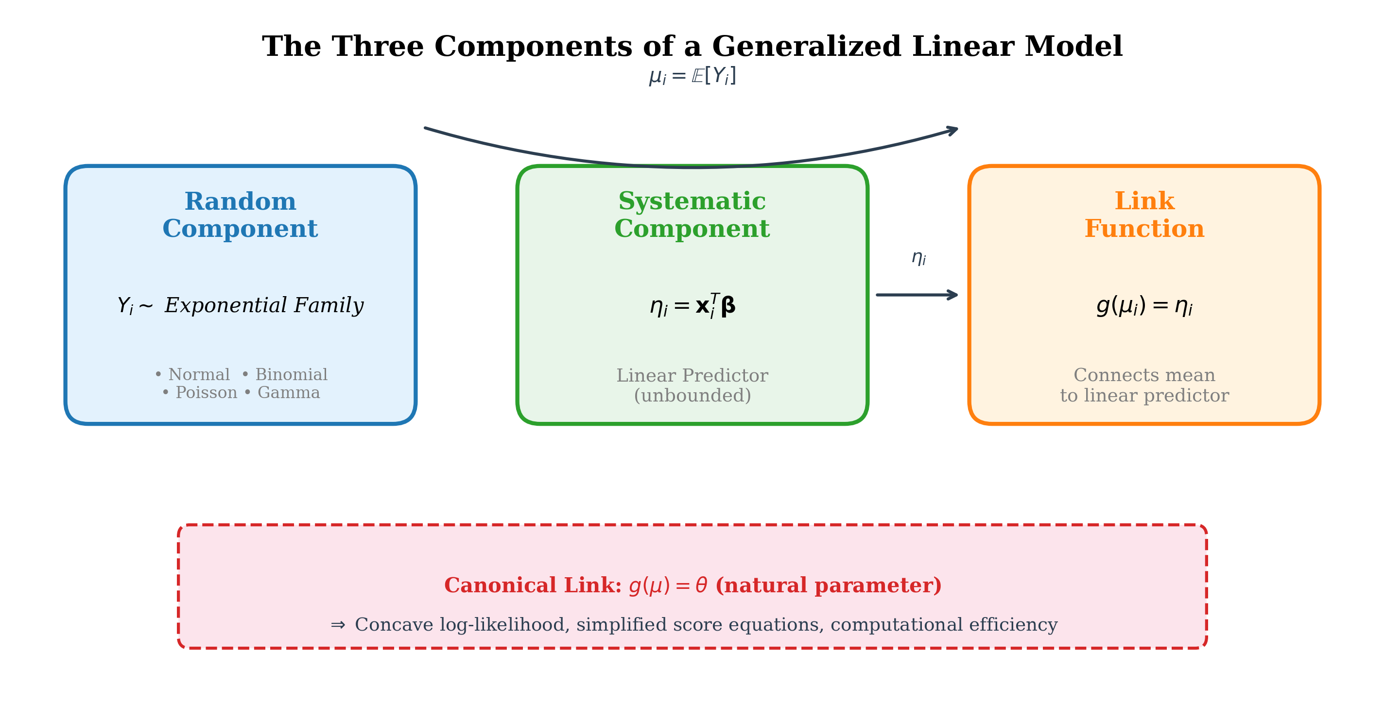
Fig. 116 Figure 3.5.1: The three-component GLM framework. The random component specifies the distribution of \(Y\) (exponential family). The systematic component combines predictors linearly into \(\eta = \mathbf{X}\boldsymbol{\beta}\). The link function \(g\) connects them: \(g(\mu) = \eta\). The canonical link sets \(\eta = \theta\), yielding computational simplifications.
Score Equations and Fisher Information
Maximum likelihood estimation for GLMs requires solving a system of nonlinear equations. In this section, we derive the score function and Fisher information matrix, which form the foundation for the IRLS algorithm.
The Log-Likelihood
For \(n\) independent observations \((y_i, \mathbf{x}_i)\), the log-likelihood is:
where \(\theta_i = \theta(\mu_i)\) and \(\mu_i = g^{-1}(\mathbf{x}_i^\top\boldsymbol{\beta})\). The parameter \(\boldsymbol{\beta}\) enters through the chain:
Deriving the Score Function
The score function is the gradient of the log-likelihood with respect to \(\boldsymbol{\beta}\). Applying the chain rule:
Let us compute each factor:
Derivative with respect to \(\theta_i\):
\[\frac{\partial \ell_i}{\partial \theta_i} = \frac{y_i - b'(\theta_i)}{\phi} = \frac{y_i - \mu_i}{\phi}\]since \(\mu_i = b'(\theta_i)\).
Derivative of \(\theta_i\) with respect to \(\mu_i\):
Since \(\mu = b'(\theta)\), by inverse function differentiation:
\[\frac{\partial \theta_i}{\partial \mu_i} = \frac{1}{b''(\theta_i)} = \frac{1}{V(\mu_i)}\]Derivative of \(\mu_i\) with respect to \(\eta_i\):
\[\frac{\partial \mu_i}{\partial \eta_i} = \frac{1}{g'(\mu_i)}\]where \(g'(\mu)\) is the derivative of the link function.
Derivative of \(\eta_i\) with respect to \(\beta_j\):
\[\frac{\partial \eta_i}{\partial \beta_j} = x_{ij}\]
Combining these:
Define the working weight for observation \(i\):
Then the score equations \(\partial \ell / \partial \beta_j = 0\) become:
Note: Different Conventions in the Literature
Different authors package the weight factor differently. Some texts write \(\sum_i (y_i - \mu_i) (\partial\mu_i/\partial\eta_i) x_{ij} / [V(\mu_i)\phi]\), others use \(\mathbf{X}^\top \mathbf{W} (\mathbf{y} - \boldsymbol{\mu})\) where \(\mathbf{W}\) absorbs all variance and derivative terms. Our formulation (110) explicitly separates the weight \(w_i\) from the link derivative \(g'(\mu_i)\), making the connection to weighted least squares transparent. When translating between sources, verify how each defines its weight matrix—the coefficient estimates will be identical, but intermediate quantities may differ.
Matrix Form of Score Equations
Define diagonal weight matrix \(\mathbf{W} = \text{diag}(w_1, \ldots, w_n)\) and the diagonal matrix of link derivatives \(\mathbf{G} = \text{diag}(g'(\mu_1), \ldots, g'(\mu_n))\). The score vector is:
The score equations \(\mathbf{U}(\boldsymbol{\beta}) = \mathbf{0}\) generalize the normal equations from linear regression. When the link is canonical, \(g'(\mu_i) = 1/V(\mu_i)\), so \(w_i \cdot g'(\mu_i) = 1/(\phi \cdot V(\mu_i) \cdot g'(\mu_i)) = 1/\phi\), and the score simplifies to:
This elegant form—residuals projected onto the column space of \(\mathbf{X}\)—directly generalizes the OLS normal equations.
Fisher Information Matrix
The Fisher information matrix is the expected negative Hessian of the log-likelihood:
For GLMs, this takes the form:
where \(\mathbf{W}\) is the diagonal weight matrix with entries \(w_i\) from (109).
Proof sketch: The second derivative of \(\ell_i\) with respect to \(\beta_j\) and \(\beta_k\) involves terms from differentiating \(\mu_i\) and \(w_i\). Taking expectations, terms involving \((y_i - \mu_i)\) vanish since \(\mathbb{E}[Y_i] = \mu_i\). The remaining terms yield \(-w_i x_{ij} x_{ik}\), and summing gives \(-[\mathbf{X}^\top\mathbf{W}\mathbf{X}]_{jk}\).
For canonical links, the observed and expected information coincide:
This equality is a consequence of the sufficient statistic being linear in \(\mathbf{y}\) and is one of the key computational advantages of canonical links.
Asymptotic Distribution of MLEs
Under standard regularity conditions, the MLE \(\hat{\boldsymbol{\beta}}\) is:
Consistent: \(\hat{\boldsymbol{\beta}} \xrightarrow{p} \boldsymbol{\beta}_0\) as \(n \to \infty\)
Asymptotically normal:
\[\sqrt{n}(\hat{\boldsymbol{\beta}} - \boldsymbol{\beta}_0) \xrightarrow{d} N(\mathbf{0}, \mathbf{I}(\boldsymbol{\beta}_0)^{-1})\]Asymptotically efficient: Achieves the Cramér-Rao lower bound.
The estimated covariance matrix is:
where \(\hat{\mathbf{W}}\) is the weight matrix evaluated at \(\hat{\boldsymbol{\beta}}\). Standard errors are the square roots of the diagonal elements.
Iteratively Reweighted Least Squares
The score equations (110) are nonlinear in \(\boldsymbol{\beta}\) because the weights \(w_i\) and means \(\mu_i\) depend on \(\boldsymbol{\beta}\). Closed-form solutions generally do not exist, so we must resort to iterative numerical methods. The standard approach is Iteratively Reweighted Least Squares (IRLS), which emerges naturally from Fisher scoring.
From Fisher Scoring to IRLS
Recall from Section 3.2 that Fisher scoring updates the parameter estimate using:
Substituting the GLM expressions for \(\mathbf{I}\) and \(\mathbf{U}\):
where superscript \((t)\) indicates evaluation at \(\boldsymbol{\beta}^{(t)}\).
Now multiply through by \(\mathbf{X}^\top \mathbf{W}^{(t)} \mathbf{X}\):
Define the working response (adjusted dependent variable):
In vector form: \(\mathbf{z}^{(t)} = \boldsymbol{\eta}^{(t)} + \mathbf{G}^{(t)}(\mathbf{y} - \boldsymbol{\mu}^{(t)})\).
Since \(\boldsymbol{\eta}^{(t)} = \mathbf{X}\boldsymbol{\beta}^{(t)}\):
This is exactly the normal equation for weighted least squares of \(\mathbf{z}^{(t)}\) on \(\mathbf{X}\) with weights \(\mathbf{W}^{(t)}\):
The IRLS Algorithm
The derivation above reveals the IRLS algorithm: at each iteration, construct a working response and weights from the current fit, then solve a weighted least squares problem.
Algorithm: Iteratively Reweighted Least Squares (IRLS)
Input: Design matrix X (n × p), response y, link function g, variance function V
       Dispersion φ, tolerance ε, maximum iterations max_iter
Output: MLE β̂, fitted means μ̂, convergence flag

1. Initialize: β⁽⁰⁾ ← starting values (e.g., from OLS on transformed y)

2. For t = 0, 1, 2, ... until convergence:

   a. Compute linear predictor: η⁽ᵗ⁾ = X β⁽ᵗ⁾

   b. Compute fitted means: μ⁽ᵗ⁾ = g⁻¹(η⁽ᵗ⁾)

   c. Compute weights: w_i⁽ᵗ⁾ = 1 / [φ · V(μ_i⁽ᵗ⁾) · (g'(μ_i⁽ᵗ⁾))²]
      W⁽ᵗ⁾ = diag(w₁⁽ᵗ⁾, ..., wₙ⁽ᵗ⁾)

   d. Compute working response: z_i⁽ᵗ⁾ = η_i⁽ᵗ⁾ + (y_i - μ_i⁽ᵗ⁾) · g'(μ_i⁽ᵗ⁾)

   e. Solve weighted least squares:
      β⁽ᵗ⁺¹⁾ = (X'W⁽ᵗ⁾X)⁻¹ X'W⁽ᵗ⁾ z⁽ᵗ⁾

   f. Check convergence: if ||β⁽ᵗ⁺¹⁾ - β⁽ᵗ⁾|| / ||β⁽ᵗ⁾|| < ε, stop

   g. Check iteration limit: if t ≥ max_iter, warn and stop

3. Return β̂ = β⁽ᵗ⁺¹⁾, μ̂ = g⁻¹(X β̂), converged = (t < max_iter)
Computational Complexity: Each iteration requires \(O(np^2)\) operations for forming \(\mathbf{X}^\top\mathbf{W}\mathbf{X}\) and \(O(p^3)\) for solving the linear system. Total complexity is \(O(T(np^2 + p^3))\) where \(T\) is the number of iterations. For well-behaved problems, \(T\) is typically 3-8.
Convergence Properties
IRLS inherits the convergence properties of Fisher scoring:
Quadratic convergence near the solution for canonical links: the number of correct digits roughly doubles per iteration.
Global convergence for canonical links when the MLE exists: the log-likelihood is concave, so any starting point eventually reaches the global maximum.
Local convergence for non-canonical links: convergence is guaranteed only in a neighborhood of the MLE. Poor starting values may cause divergence.
Typical stopping criteria include:
Relative parameter change: \(\|\boldsymbol{\beta}^{(t+1)} - \boldsymbol{\beta}^{(t)}\| / \|\boldsymbol{\beta}^{(t)}\| < 10^{-8}\)
Relative deviance change: \(|D^{(t+1)} - D^{(t)}| / |D^{(t)}| < 10^{-8}\)
Score norm: \(\|\mathbf{U}(\boldsymbol{\beta}^{(t)})\| < 10^{-6}\)
Numerical Stability Considerations
Several issues can cause IRLS to fail or produce unreliable results:
Extreme weights: When fitted probabilities approach 0 or 1 in logistic regression, the variance \(V(\mu) = \mu(1-\mu)\) approaches 0, causing weights \(w_i \to \infty\). Simultaneously, the working response \(z_i\) can become extremely large. This typically signals separation (discussed below).
Ill-conditioned \(\mathbf{X}^\top\mathbf{W}\mathbf{X}\): Multicollinearity or extreme weight variations can make the weighted normal equations numerically unstable. QR decomposition is more stable than forming and inverting \(\mathbf{X}^\top\mathbf{W}\mathbf{X}\) directly.
Boundary parameters: When the MLE lies at or near the boundary of the parameter space (e.g., a coefficient approaching \(\pm\infty\)), standard algorithms struggle.
Common remedies include:
Step-halving: If the deviance increases, reduce the step size by half until improvement occurs
Ridge stabilization: Add \(\lambda\mathbf{I}\) to \(\mathbf{X}^\top\mathbf{W}\mathbf{X}\) for small \(\lambda > 0\)
Bound predictions: Clip fitted probabilities to \([\epsilon, 1-\epsilon]\) for small \(\epsilon\)
QR decomposition: Solve the weighted least squares problem via QR rather than normal equations
Python Implementation
The following implementation demonstrates IRLS for a generic GLM:
import numpy as np
from scipy import linalg
from typing import Callable, Tuple, NamedTuple

class GLMFamily(NamedTuple):
    """Specification of a GLM family."""
    name: str
    variance: Callable[[np.ndarray], np.ndarray]  # V(μ)
    link: Callable[[np.ndarray], np.ndarray]       # g(μ)
    link_deriv: Callable[[np.ndarray], np.ndarray] # g'(μ)
    link_inv: Callable[[np.ndarray], np.ndarray]   # g⁻¹(η)

# Define common families
BINOMIAL = GLMFamily(
    name='binomial',
    variance=lambda mu: mu * (1 - mu),
    link=lambda mu: np.log(mu / (1 - mu)),          # logit
    link_deriv=lambda mu: 1 / (mu * (1 - mu)),
    link_inv=lambda eta: 1 / (1 + np.exp(-eta))     # sigmoid
)

POISSON = GLMFamily(
    name='poisson',
    variance=lambda mu: mu,
    link=lambda mu: np.log(mu),                      # log
    link_deriv=lambda mu: 1 / mu,
    link_inv=lambda eta: np.exp(eta)
)

GAMMA_LOG = GLMFamily(
    name='gamma',
    variance=lambda mu: mu**2,
    link=lambda mu: np.log(mu),                      # log (not canonical)
    link_deriv=lambda mu: 1 / mu,
    link_inv=lambda eta: np.exp(eta)
)

def irls_fit(X: np.ndarray, y: np.ndarray, family: GLMFamily,
             phi: float = 1.0, tol: float = 1e-8, max_iter: int = 25,
             verbose: bool = False) -> Tuple[np.ndarray, np.ndarray, int]:
    """
    Fit a GLM using Iteratively Reweighted Least Squares.

    Parameters
    ----------
    X : ndarray of shape (n, p)
        Design matrix (should include intercept column if desired)
    y : ndarray of shape (n,)
        Response vector
    family : GLMFamily
        GLM family specification
    phi : float
        Dispersion parameter (1 for binomial/Poisson)
    tol : float
        Convergence tolerance for relative parameter change
    max_iter : int
        Maximum number of iterations
    verbose : bool
        Print iteration information

    Returns
    -------
    beta : ndarray of shape (p,)
        Estimated coefficients
    mu : ndarray of shape (n,)
        Fitted means
    n_iter : int
        Number of iterations performed
    """
    n, p = X.shape

    # Initialize: use simple starting values
    # For binomial: start with empirical proportions
    # For Poisson/Gamma: start with log of y (adjusted for zeros)
    if family.name == 'binomial':
        mu = np.clip(y, 0.01, 0.99)
    else:
        mu = np.maximum(y, 0.1)

    eta = family.link(mu)
    beta = np.linalg.lstsq(X, eta, rcond=None)[0]

    for iteration in range(max_iter):
        # Current linear predictor and mean
        eta = X @ beta
        mu = family.link_inv(eta)

        # Numerical safeguards
        if family.name == 'binomial':
            mu = np.clip(mu, 1e-10, 1 - 1e-10)
        else:
            mu = np.maximum(mu, 1e-10)

        # Compute weights: w = 1 / [φ * V(μ) * (g'(μ))²]
        V = family.variance(mu)
        g_prime = family.link_deriv(mu)
        w = 1 / (phi * V * g_prime**2)

        # Compute working response: z = η + (y - μ) * g'(μ)
        z = eta + (y - mu) * g_prime

        # Weighted least squares update
        W_sqrt = np.sqrt(w)
        X_tilde = X * W_sqrt[:, np.newaxis]  # √W X
        z_tilde = z * W_sqrt                  # √W z

        # Solve via QR for numerical stability
        beta_new, _, _, _ = np.linalg.lstsq(X_tilde, z_tilde, rcond=None)

        # Check convergence
        relative_change = np.linalg.norm(beta_new - beta) / (np.linalg.norm(beta) + 1e-10)

        if verbose:
            deviance = compute_deviance(y, mu, family, phi)
            print(f"Iteration {iteration + 1}: deviance = {deviance:.6f}, "
                  f"relative change = {relative_change:.2e}")

        beta = beta_new

        if relative_change < tol:
            if verbose:
                print(f"Converged after {iteration + 1} iterations")
            return beta, family.link_inv(X @ beta), iteration + 1

    print(f"Warning: IRLS did not converge after {max_iter} iterations")
    return beta, family.link_inv(X @ beta), max_iter

def compute_deviance(y: np.ndarray, mu: np.ndarray,
                     family: GLMFamily, phi: float = 1.0) -> float:
    """Compute the deviance for a fitted GLM."""
    # Avoid log(0) issues
    eps = 1e-10

    if family.name == 'binomial':
        # D = 2 Σ [y log(y/μ) + (1-y) log((1-y)/(1-μ))]
        y_safe = np.clip(y, eps, 1 - eps)
        mu_safe = np.clip(mu, eps, 1 - eps)
        d = 2 * np.sum(
            y * np.log(y_safe / mu_safe + eps) +
            (1 - y) * np.log((1 - y_safe) / (1 - mu_safe) + eps)
        )
    elif family.name == 'poisson':
        # D = 2 Σ [y log(y/μ) - (y - μ)]
        y_safe = np.maximum(y, eps)
        d = 2 * np.sum(y * np.log(y_safe / mu + eps) - (y - mu))
    elif family.name == 'gamma':
        # D = 2 Σ [-log(y/μ) + (y - μ)/μ]
        d = 2 * np.sum(-np.log(y / mu) + (y - mu) / mu)
    else:
        # Normal: D = Σ (y - μ)²
        d = np.sum((y - mu)**2) / phi

    return d
Example 💡 IRLS Convergence for Logistic Regression
Given: Simulated binary data with known coefficients \(\beta_0 = -2, \beta_1 = 0.5\).
Find: MLE via IRLS and observe convergence behavior.
Python implementation:
import numpy as np

# Generate data
rng = np.random.default_rng(42)
n = 200
x = rng.uniform(0, 10, n)
eta_true = -2.0 + 0.5 * x
p_true = 1 / (1 + np.exp(-eta_true))
y = rng.binomial(1, p_true)

# Design matrix with intercept
X = np.column_stack([np.ones(n), x])

# Fit via IRLS
beta_hat, mu_hat, n_iter = irls_fit(X, y, BINOMIAL, verbose=True)

print(f"\nTrue coefficients: β₀ = -2.0, β₁ = 0.5")
print(f"MLE estimates:     β₀ = {beta_hat[0]:.4f}, β₁ = {beta_hat[1]:.4f}")
print(f"Converged in {n_iter} iterations")
Result:
Iteration 1: deviance = 177.4231, relative change = 1.12e+00
Iteration 2: deviance = 169.8845, relative change = 1.67e-01
Iteration 3: deviance = 169.6012, relative change = 1.52e-02
Iteration 4: deviance = 169.5987, relative change = 1.41e-04
Iteration 5: deviance = 169.5987, relative change = 1.24e-08
Converged after 5 iterations

True coefficients: β₀ = -2.0, β₁ = 0.5
MLE estimates:     β₀ = -2.1893, β₁ = 0.5207
Converged in 5 iterations
The rapid convergence—relative change dropping from \(10^0\) to \(10^{-8}\) in just 5 iterations—demonstrates the quadratic convergence of IRLS for the canonical logit link.
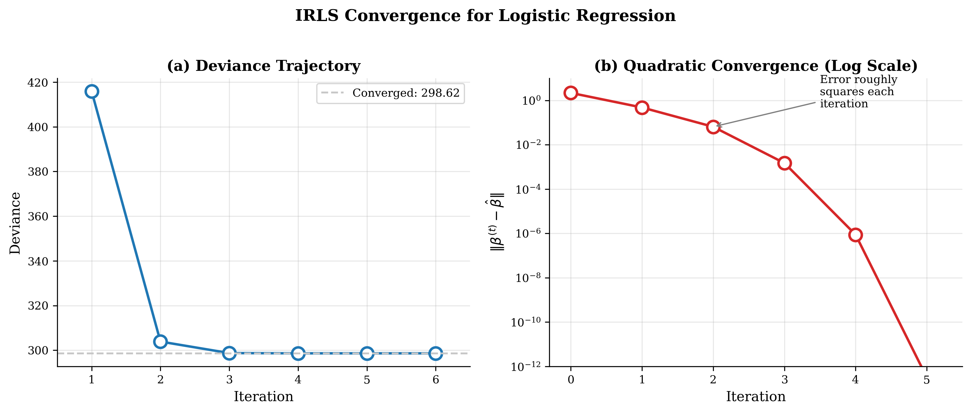
Fig. 117 Figure 3.5.2: IRLS convergence for logistic regression. (a) Deviance decreases monotonically, approaching the minimum in few iterations. (b) Log-scale error \(\log_{10}|\boldsymbol{\beta}^{(t)} - \hat{\boldsymbol{\beta}}|\) shows quadratic convergence—the slope doubles each iteration, meaning the number of correct digits roughly doubles.
Logistic Regression: Binary Outcomes
Logistic regression is the most widely used GLM, modeling binary outcomes (yes/no, success/failure, 0/1) as functions of predictors. Its applications span medicine (disease diagnosis), marketing (customer churn), finance (credit default), and countless other domains.
Model Specification
For binary responses \(Y_i \in \{0, 1\}\), we model \(Y_i \sim \text{Bernoulli}(\pi_i)\) where \(\pi_i = P(Y_i = 1 | \mathbf{x}_i)\). The logit link (canonical for Bernoulli) connects \(\pi_i\) to the linear predictor:
The quantity \(\pi_i / (1 - \pi_i)\) is the odds of success—the ratio of the probability of success to the probability of failure. The logit is the log-odds.
Inverting the link gives the logistic function (sigmoid):
The S-shaped logistic curve maps the unbounded linear predictor \(\eta \in (-\infty, \infty)\) to the probability interval \(\pi \in (0, 1)\).
For the Bernoulli distribution:
Variance function: \(V(\pi) = \pi(1 - \pi)\)
Dispersion: \(\phi = 1\) (fixed, not estimated)
Weight: \(w_i = \pi_i(1 - \pi_i)\) (for canonical logit link)
Interpretation: Odds Ratios
Logistic regression coefficients have a natural interpretation in terms of odds ratios. Consider a single predictor:
For two values \(x\) and \(x + 1\):
Exponentiating:
Thus \(e^{\beta_1}\) is the multiplicative change in odds for a one-unit increase in \(x\). If \(\beta_1 = 0.5\), then \(e^{0.5} \approx 1.65\): each unit increase in \(x\) multiplies the odds by 1.65 (a 65% increase).
For categorical predictors with dummy coding, \(e^{\beta_j}\) is the odds ratio comparing category \(j\) to the reference category.
In multiple logistic regression, each \(e^{\beta_j}\) is an adjusted odds ratio—the multiplicative change in odds per unit increase in \(x_j\), holding all other predictors constant.
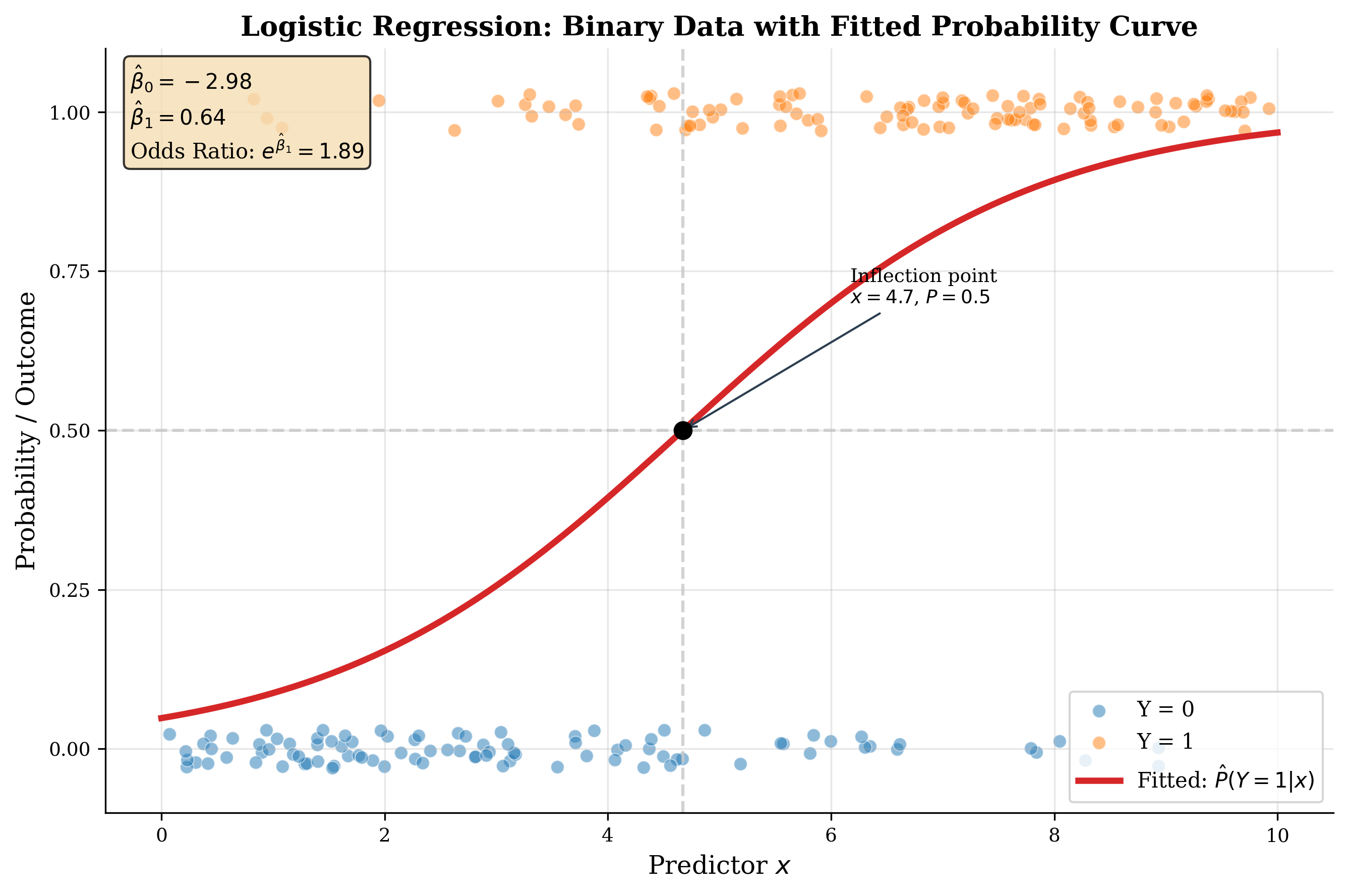
Fig. 118 Figure 3.5.3: Logistic regression with simulated data. Points show binary outcomes \(y \in \{0, 1\}\) (jittered vertically for visibility). The S-shaped curve is the fitted probability \(\hat{\pi}(x) = 1/(1 + e^{-\hat{\eta}})\). As \(x\) increases, the probability transitions smoothly from near 0 to near 1. The inflection point occurs where \(\hat{\eta} = 0\), i.e., \(x = -\hat{\beta}_0/\hat{\beta}_1\).
The Separation Problem
A unique challenge in logistic regression is separation—when a linear combination of predictors perfectly predicts the binary outcome. When this occurs, the MLE does not exist in the usual sense: coefficients diverge to \(\pm\infty\) while the likelihood continues increasing.
Complete separation occurs when the classes can be perfectly separated by a hyperplane:
for some \(\boldsymbol{\beta}\). In this case, scaling \(\boldsymbol{\beta} \to c\boldsymbol{\beta}\) with \(c \to \infty\) drives all predicted probabilities toward their observed values (0 or 1), and the log-likelihood approaches 0 from below.
Quasi-complete separation occurs when separation exists only at boundary points—some observations lie exactly on the separating hyperplane.
Symptoms of separation:
Very large coefficient estimates (\(|\hat{\beta}| > 10\))
Extremely large standard errors (sometimes reported as infinity)
Convergence warnings or failure to converge
Fitted probabilities exactly 0 or 1
Firth’s Penalized Likelihood
David Firth (1993) proposed a penalized likelihood that removes first-order bias and produces finite estimates even under separation:
The penalty \(\frac{1}{2}\log|\mathbf{I}(\boldsymbol{\beta})|\) is the Jeffreys prior in Bayesian terms. The modified score equations are:
For logistic regression, this simplifies to adding a term involving the hat matrix diagonal \(h_{ii}\):
Firth’s method is not available as a built-in option in standard Python libraries like statsmodels or sklearn. For production use, implement the modified score equations directly as shown in Exercise 3.5.3, use L2 regularization (LogisticRegression(penalty='l2', C=10)) as a practical approximation, or install the firthlogist package from PyPI which provides a pure Python implementation.
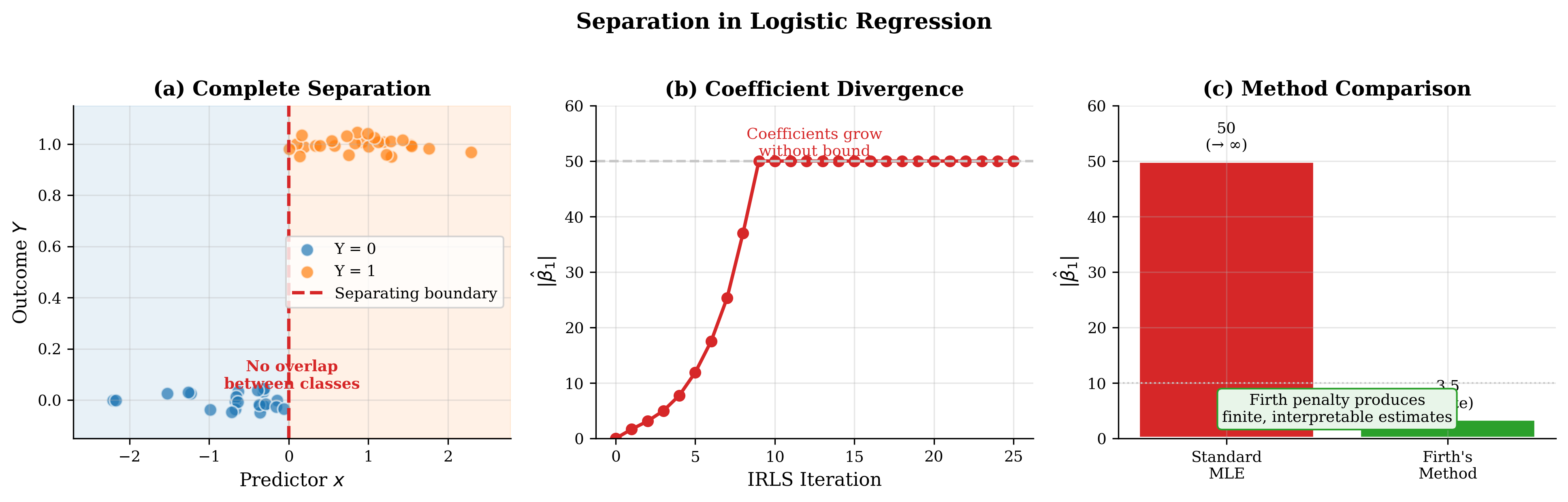
Fig. 119 Figure 3.5.4: Separation in logistic regression. (a) Separable data: all \(y=1\) cases have \(x > 5\), all \(y=0\) cases have \(x < 5\). No finite MLE exists. (b) Coefficient estimates vs. iteration: \(|\hat{\beta}_1|\) grows without bound as IRLS attempts to achieve perfect separation. (c) Standard MLE produces infinite coefficients; Firth’s method produces finite, interpretable estimates.
Worked Example: Logistic Regression in Python
import numpy as np
import statsmodels.api as sm
from sklearn.linear_model import LogisticRegression
import matplotlib.pyplot as plt

# Generate data
rng = np.random.default_rng(42)
n = 200
x = rng.uniform(0, 10, n)
eta_true = -3.0 + 0.6 * x
p_true = 1 / (1 + np.exp(-eta_true))
y = rng.binomial(1, p_true)

# Fit with statsmodels
X_sm = sm.add_constant(x)
logit_model = sm.GLM(y, X_sm, family=sm.families.Binomial())
result = logit_model.fit()

print("=== Statsmodels GLM Results ===")
print(result.summary())

# Extract key results
print(f"\nCoefficients: β₀ = {result.params[0]:.4f}, β₁ = {result.params[1]:.4f}")
print(f"Standard errors: SE(β₀) = {result.bse[0]:.4f}, SE(β₁) = {result.bse[1]:.4f}")
print(f"Odds ratio for x: exp(β₁) = {np.exp(result.params[1]):.4f}")
print(f"Deviance: {result.deviance:.4f}")
print(f"AIC: {result.aic:.4f}")

# Fit with scikit-learn (for comparison)
clf = LogisticRegression(penalty=None, solver='lbfgs')
clf.fit(x.reshape(-1, 1), y)

print(f"\n=== Scikit-learn Results ===")
print(f"Coefficients: β₀ = {clf.intercept_[0]:.4f}, β₁ = {clf.coef_[0, 0]:.4f}")

# Predictions
x_pred = np.linspace(0, 10, 100)
X_pred = sm.add_constant(x_pred)
p_pred = result.predict(X_pred)

# Plot
fig, ax = plt.subplots(figsize=(8, 5))
ax.scatter(x, y + rng.uniform(-0.02, 0.02, n), alpha=0.5, label='Data')
ax.plot(x_pred, p_pred, 'r-', linewidth=2, label='Fitted probability')
ax.axhline(0.5, color='gray', linestyle='--', alpha=0.5)
ax.axvline(-result.params[0]/result.params[1], color='gray', linestyle='--', alpha=0.5)
ax.set_xlabel('x')
ax.set_ylabel('P(Y = 1)')
ax.set_title('Logistic Regression Fit')
ax.legend()
plt.tight_layout()
plt.savefig('logistic_fit.png', dpi=150)
Poisson Regression: Count Data
Poisson regression models count outcomes—non-negative integers representing the number of events occurring in a fixed period or region. Applications include modeling the number of insurance claims, website visits, disease cases, or manufacturing defects.
Model Specification
For count responses \(Y_i \in \{0, 1, 2, \ldots\}\), we model \(Y_i \sim \text{Poisson}(\mu_i)\). The log link (canonical for Poisson) connects \(\mu_i\) to the linear predictor:
Equivalently:
This ensures \(\mu_i > 0\) as required for a Poisson mean.
For the Poisson distribution:
Variance function: \(V(\mu) = \mu\)
Dispersion: \(\phi = 1\) (fixed)
Weight: \(w_i = \mu_i\) (for canonical log link)
The Poisson assumption implies \(\text{Var}(Y_i) = \mathbb{E}[Y_i] = \mu_i\)—the variance equals the mean. This equidispersion property is often violated in practice.
Interpretation: Rate Ratios
Poisson regression coefficients have multiplicative interpretations. For a single predictor:
Exponentiating:
Thus \(e^{\beta_1}\) is the multiplicative change in expected count for a one-unit increase in \(x\). If \(\beta_1 = 0.3\), then \(e^{0.3} \approx 1.35\): each unit increase in \(x\) multiplies the expected count by 1.35 (a 35% increase).
Offsets for Rate Modeling
Often we model rates rather than raw counts. If \(Y_i\) is the count and \(t_i\) is the exposure (time period, population size, area), then:
where \(\lambda_i\) is the rate. Taking logarithms:
The term \(\log(t_i)\) is called an offset—it enters the linear predictor with coefficient fixed at 1. In software:
# Statsmodels
model = sm.GLM(counts, X, family=sm.families.Poisson(),
               offset=np.log(exposure))
The Overdispersion Problem
Real count data often exhibits overdispersion: \(\text{Var}(Y_i) > \mathbb{E}[Y_i]\). Causes include:
Unobserved heterogeneity: Unmeasured factors cause variation in rates across observations
Clustering: Observations within groups are correlated
Zero-inflation: Excess zeros beyond what Poisson predicts
Detecting overdispersion: Compare the Pearson chi-square statistic to its degrees of freedom:
Under correct specification, \(\hat{\phi} \approx 1\). Values substantially greater than 1 indicate overdispersion.
Consequences of ignoring overdispersion:
Standard errors are too small
Confidence intervals are too narrow
p-values are too small
Type I error rate inflated
Remedies:
Quasi-Poisson: Estimate \(\phi\) from data and inflate standard errors by \(\sqrt{\hat{\phi}}\)
Negative Binomial regression: Model \(Y_i \sim \text{NegBin}(\mu_i, \alpha)\) with \(\text{Var}(Y_i) = \mu_i + \alpha\mu_i^2\)
Robust standard errors: Use sandwich estimator (see Section 3.5.10)
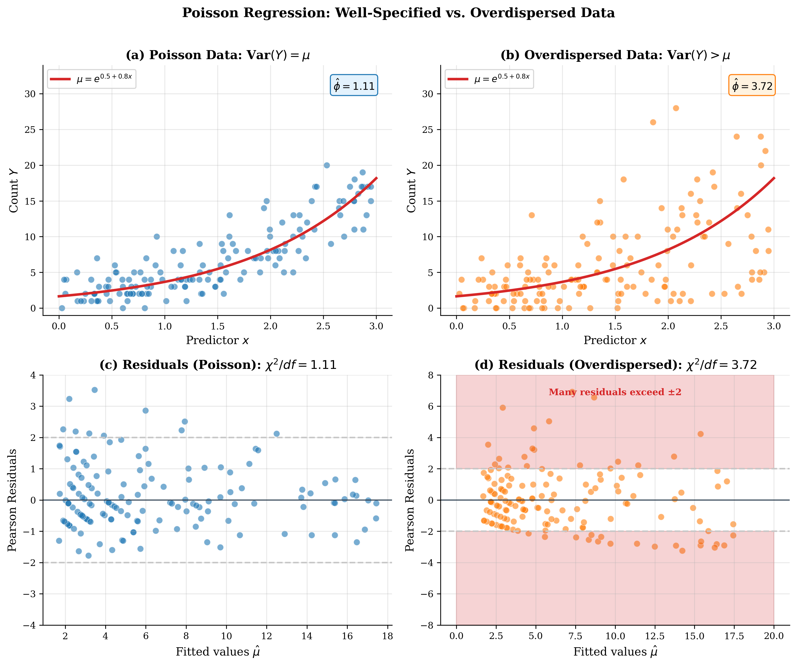
Fig. 120 Figure 3.5.5: Poisson regression and overdispersion. (a) Well-behaved Poisson data: variance approximately equals mean, residuals show no pattern. (b) Overdispersed data: variance exceeds mean, Pearson \(\chi^2/\text{df} = 3.2\). Standard Poisson SEs are too small; quasi-Poisson or negative binomial provides correct inference.
Worked Example: Poisson Regression
import numpy as np
import statsmodels.api as sm

# Generate Poisson data
rng = np.random.default_rng(101)
n = 150
x = rng.uniform(0, 3, n)
mu_true = np.exp(0.5 + 0.8 * x)
y = rng.poisson(mu_true)

# Fit Poisson GLM
X = sm.add_constant(x)
poisson_model = sm.GLM(y, X, family=sm.families.Poisson())
result = poisson_model.fit()

print("=== Poisson Regression Results ===")
print(f"Coefficients: β₀ = {result.params[0]:.4f}, β₁ = {result.params[1]:.4f}")
print(f"True values:  β₀ = 0.5000, β₁ = 0.8000")
print(f"\nRate ratio for x: exp(β₁) = {np.exp(result.params[1]):.4f}")
print(f"(Each unit increase in x multiplies expected count by {np.exp(result.params[1]):.2f})")

# Check for overdispersion
pearson_chi2 = result.pearson_chi2
df_resid = result.df_resid
phi_hat = pearson_chi2 / df_resid

print(f"\n=== Overdispersion Check ===")
print(f"Pearson χ²: {pearson_chi2:.2f}")
print(f"Degrees of freedom: {df_resid}")
print(f"Estimated φ = χ²/df: {phi_hat:.3f}")
print(f"Conclusion: {'Overdispersion detected' if phi_hat > 1.5 else 'No strong overdispersion'}")
Gamma Regression: Positive Continuous Data
Gamma regression models positive continuous responses, particularly when variance increases with the mean. It is widely used in insurance (claim amounts), reliability engineering (failure times), and economics (income, costs).
Model Specification
For positive continuous \(Y_i > 0\), we model \(Y_i \sim \text{Gamma}(\alpha, \mu_i)\) with shape \(\alpha\) and mean \(\mu_i\). The variance is:
where \(\phi = 1/\alpha\) is the dispersion parameter. This implies a constant coefficient of variation:
The canonical link for Gamma is the inverse \(g(\mu) = -1/\mu\), but the log link is almost always preferred:
The log link ensures \(\mu_i > 0\) and provides multiplicative coefficient interpretations, just as in Poisson regression.
For the Gamma distribution with log link:
Variance function: \(V(\mu) = \mu^2\)
Dispersion: \(\phi = 1/\alpha\) (estimated from data)
Weight factor: \(V(\mu) \cdot (g'(\mu))^2 = \mu^2 \cdot (1/\mu)^2 = 1\), so \(w_i = 1/\phi\) for all \(i\)
The key insight is that weights do not vary across observations—a constant multiplier on all weights does not change the WLS coefficient solution, so IRLS behaves like unweighted least squares on the working response (though standard errors still depend on \(\phi\)).
Interpretation
With a log link, \(e^{\beta_j}\) is the multiplicative change in expected response for a one-unit increase in \(x_j\):
If \(\beta_1 = 0.4\), then \(e^{0.4} \approx 1.49\): each unit increase multiplies the expected response by 1.49 (a 49% increase).
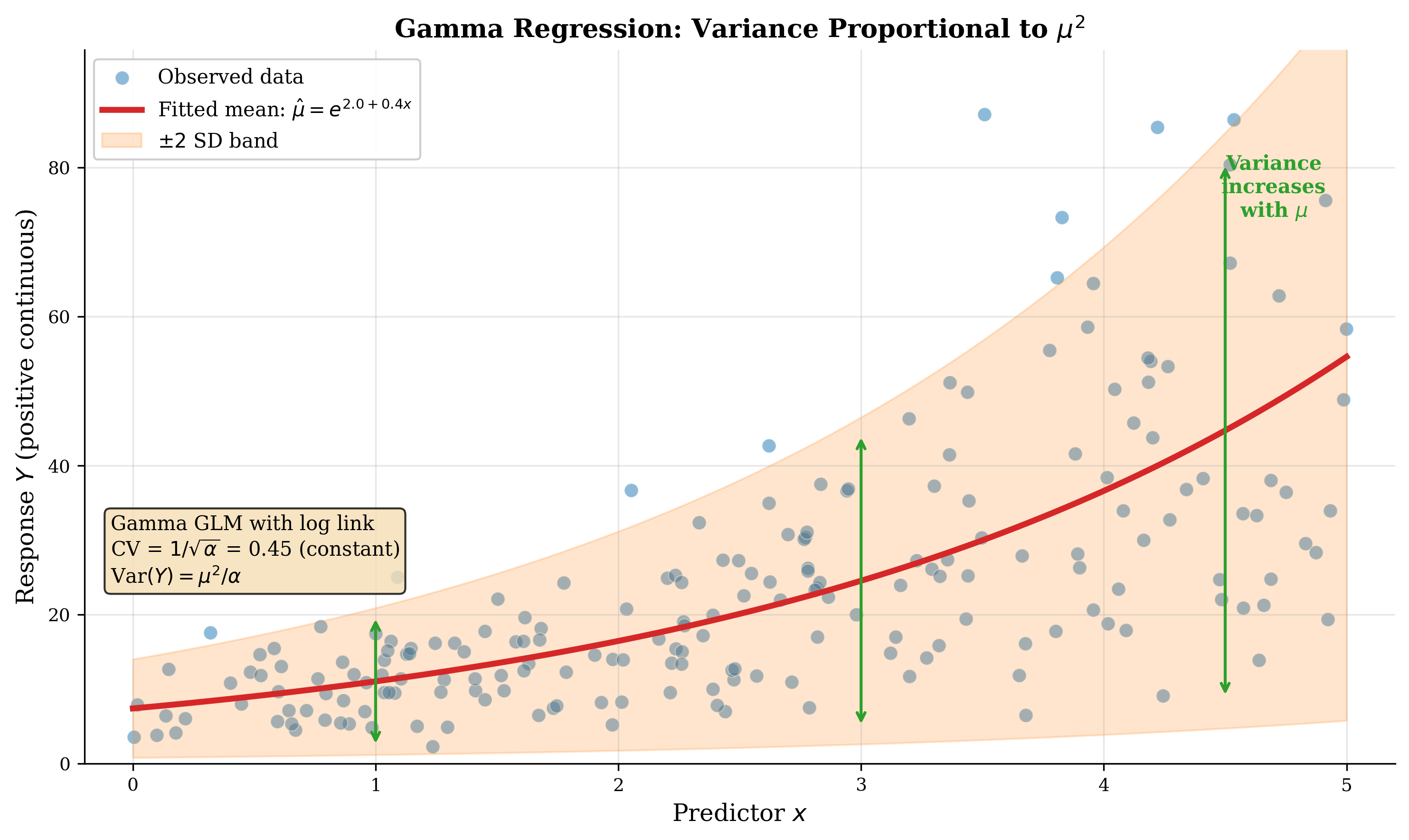
Fig. 121 Figure 3.5.6: Gamma regression for positive continuous data. The exponential mean function \(\hat{\mu}(x) = \exp(\hat{\beta}_0 + \hat{\beta}_1 x)\) fits the data well. Note how the spread of observations increases with \(x\)—this heteroskedasticity (variance proportional to \(\mu^2\)) is exactly what the Gamma model accommodates.
Worked Example: Gamma Regression
import numpy as np
import statsmodels.api as sm

# Generate Gamma data
rng = np.random.default_rng(202)
n = 200
x = rng.uniform(0, 5, n)
mu_true = np.exp(2.0 + 0.4 * x)
alpha = 5.0  # shape parameter
y = rng.gamma(shape=alpha, scale=mu_true / alpha)

# Fit Gamma GLM with log link
X = sm.add_constant(x)
gamma_model = sm.GLM(y, X,
                     family=sm.families.Gamma(link=sm.families.links.Log()))
result = gamma_model.fit()

print("=== Gamma Regression Results ===")
print(f"Coefficients: β₀ = {result.params[0]:.4f}, β₁ = {result.params[1]:.4f}")
print(f"True values:  β₀ = 2.0000, β₁ = 0.4000")
print(f"\nMultiplicative effect: exp(β₁) = {np.exp(result.params[1]):.4f}")
print(f"Estimated dispersion φ: {result.scale:.4f}")
print(f"True dispersion 1/α:    {1/alpha:.4f}")
Inference in GLMs: The Testing Triad
Three classical approaches to hypothesis testing are available for GLMs: Wald tests, likelihood ratio tests, and score tests. All three are asymptotically equivalent under the null hypothesis but can differ substantially in finite samples.
Wald Tests
The Wald test exploits the asymptotic normality of \(\hat{\boldsymbol{\beta}}\). For testing \(H_0: \beta_j = 0\):
For testing multiple parameters \(H_0: \mathbf{C}\boldsymbol{\beta} = \mathbf{d}\):
where \(q = \text{rank}(\mathbf{C})\).
Advantages: Requires only the fitted model (no need to fit reduced models).
Disadvantages:
Not invariant to reparameterization
Can behave poorly near parameter boundaries (Hauck-Donner effect)
Less accurate than LRT in small samples
Likelihood Ratio Tests
The likelihood ratio test (LRT) compares nested models directly:
where \(q\) is the difference in number of parameters.
For GLMs, this equals the difference in deviances between models.
Advantages:
Invariant to reparameterization
Generally more accurate than Wald in finite samples
Natural interpretation as deviance reduction
Disadvantages:
Requires fitting both full and reduced models
Score Tests
The score test (Rao test) evaluates whether the score function is significantly different from zero when evaluated at the null hypothesis:
where \(\boldsymbol{\beta}_0\) is the parameter value under \(H_0\).
Advantages:
Requires only the null model
Efficient for screening many potential predictors
Useful when full model is difficult to fit
Disadvantages:
Requires computing score and information under null
Asymptotic Equivalence
Under standard regularity conditions and the null hypothesis:
All three statistics converge to the same \(\chi^2_q\) distribution. In linear models with known variance, there is an ordering: \(W \geq \Lambda \geq S\).
Practical Guidance
Default choice: Use the likelihood ratio test for its accuracy and invariance
Quick screening: Use Wald tests from model summary output
Difficult full models: Use score test when the alternative model is hard to fit
Near boundaries/separation: Prefer LRT or score over Wald
Worked Example: Comparing Tests
import numpy as np
import statsmodels.api as sm
from scipy import stats

# Generate data
rng = np.random.default_rng(123)
n = 100
x1 = rng.normal(0, 1, n)
x2 = rng.normal(0, 1, n)
eta = -1 + 0.8 * x1 + 0.3 * x2
p = 1 / (1 + np.exp(-eta))
y = rng.binomial(1, p)

# Fit full and reduced models
X_full = sm.add_constant(np.column_stack([x1, x2]))
X_reduced = sm.add_constant(x1)

model_full = sm.GLM(y, X_full, family=sm.families.Binomial()).fit()
model_reduced = sm.GLM(y, X_reduced, family=sm.families.Binomial()).fit()

# Test H0: β₂ = 0

# 1. Wald test (from full model)
z_wald = model_full.params[2] / model_full.bse[2]
p_wald = 2 * (1 - stats.norm.cdf(np.abs(z_wald)))

# 2. Likelihood ratio test
lr_stat = model_reduced.deviance - model_full.deviance
p_lrt = 1 - stats.chi2.cdf(lr_stat, df=1)

print("=== Testing H₀: β₂ = 0 ===")
print(f"\nWald test:     z = {z_wald:.4f}, p = {p_wald:.4f}")
print(f"LR test:       χ² = {lr_stat:.4f}, p = {p_lrt:.4f}")
print(f"\nTrue β₂ = 0.3 (not zero), so we expect to reject H₀")
Model Diagnostics
Assessing model fit is crucial for GLMs. Unlike linear regression where residuals are straightforward to interpret, GLM diagnostics require careful attention to the choice of residual type and the non-constant variance structure.
Deviance and Model Fit
The deviance measures how far the fitted model is from a saturated model (one parameter per observation):
Each observation contributes a unit deviance \(d_i\):
Distribution |
Unit Deviance \(d_i\) |
|---|---|
Normal |
\((y_i - \hat{\mu}_i)^2\) |
Binomial |
\(2[y_i \log(y_i/\hat{\pi}_i) + (1-y_i)\log((1-y_i)/(1-\hat{\pi}_i))]\) |
Poisson |
\(2[y_i \log(y_i/\hat{\mu}_i) - (y_i - \hat{\mu}_i)]\) |
Gamma |
\(2[-\log(y_i/\hat{\mu}_i) + (y_i - \hat{\mu}_i)/\hat{\mu}_i]\) |
The total deviance is \(D = \sum_i d_i\).
Deviance as goodness-of-fit: Under correct specification with grouped data or large counts, \(D \sim \chi^2_{n-p}\) approximately. Thus \(D/(n-p) \approx 1\) indicates adequate fit. However, this approximation fails for ungrouped binary data—use the Hosmer-Lemeshow test instead.
Comparing nested models: For models \(M_0 \subset M_1\):
under \(H_0\) that the reduced model is adequate.
Residual Types
Several residual types are available for GLMs:
Pearson residuals:
These have approximately unit variance under correct specification. Their sum of squares gives the Pearson \(\chi^2\) statistic: \(X^2 = \sum_i (r_i^P)^2\).
Deviance residuals:
These are defined so \(\sum_i (r_i^D)^2 = D\). Deviance residuals are often more symmetric than Pearson residuals, especially for skewed response distributions.
Standardized residuals adjust for leverage:
where \(h_{ii}\) is the \(i\)-th diagonal of the hat matrix \(\mathbf{H} = \mathbf{W}^{1/2}\mathbf{X}(\mathbf{X}^\top\mathbf{W}\mathbf{X})^{-1}\mathbf{X}^\top\mathbf{W}^{1/2}\).
Diagnostic Plots
Standard diagnostic plots for GLMs include:
Residuals vs. fitted values: Look for patterns indicating model misspecification (nonlinearity, omitted variables)
Q-Q plot of deviance residuals: Check approximate normality of residuals
Scale-location plot: \(\sqrt{|r_i^D|}\) vs. fitted, checking for heteroskedasticity beyond what the model accommodates
Residuals vs. each predictor: Detect nonlinear relationships
Special case—binary outcomes: For ungrouped binary data, individual residual plots are uninformative (residuals take only two distinct values for each fitted probability). Use binned residual plots: group observations by fitted probability, compute average residual in each bin, and check if averages are approximately zero.
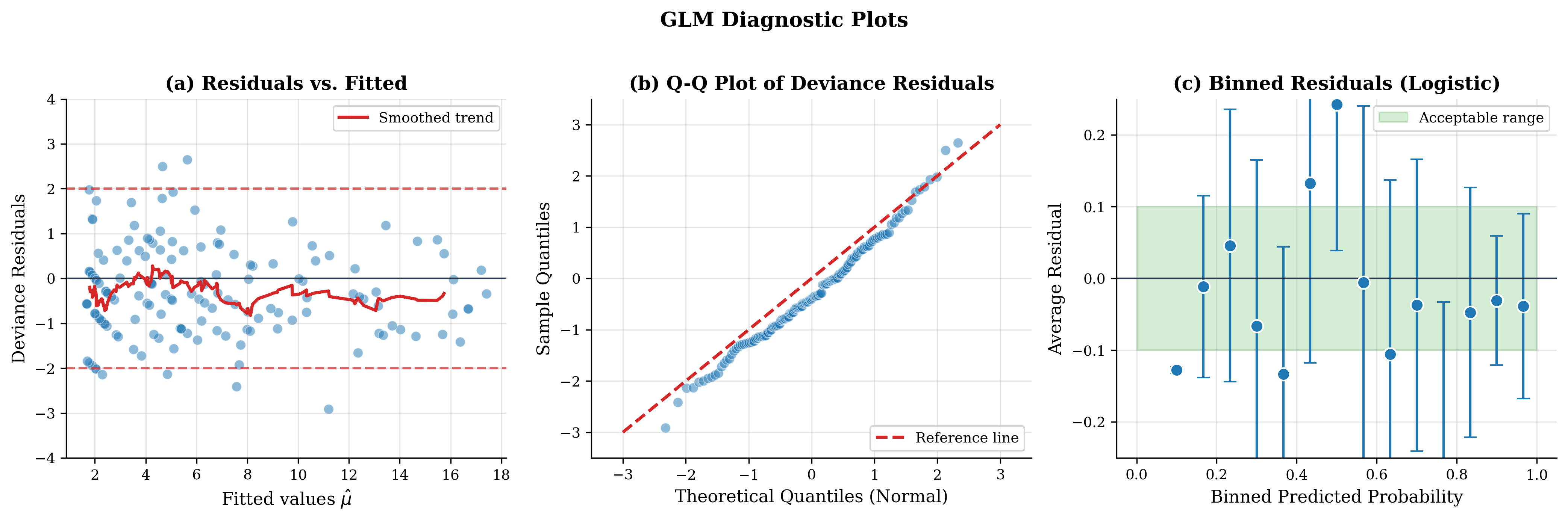
Fig. 122 Figure 3.5.7: GLM diagnostic plots for Poisson regression. (a) Deviance residuals vs. fitted values—no obvious pattern indicates adequate fit. (b) Q-Q plot of deviance residuals against standard normal quantiles—approximate linearity suggests the Poisson model is reasonable. (c) Binned residual plot for logistic regression showing average residuals within probability bins.
Model Comparison and Selection
When multiple candidate models exist, we need criteria for choosing among them.
Information Criteria
Akaike Information Criterion (AIC):
where \(p\) is the number of parameters. AIC estimates the expected Kullback-Leibler divergence and balances fit (deviance) against complexity (number of parameters). Lower AIC is better.
Bayesian Information Criterion (BIC):
BIC penalizes complexity more heavily than AIC for \(n > 7\). It is consistent: as \(n \to \infty\), BIC selects the true model with probability approaching 1 (if the true model is among candidates).
Interpretation:
\(\Delta\text{AIC} > 2\): Meaningful evidence favoring lower-AIC model
\(\Delta\text{AIC} > 10\): Strong evidence
Similar thresholds for BIC
Analysis of Deviance
For nested models, analysis of deviance tables present sequential model comparisons:
import statsmodels.api as sm

# Compare nested models
model_null = sm.GLM(y, np.ones((n, 1)), family=sm.families.Poisson()).fit()
model_x1 = sm.GLM(y, sm.add_constant(x1), family=sm.families.Poisson()).fit()
model_full = sm.GLM(y, sm.add_constant(np.column_stack([x1, x2])),
                    family=sm.families.Poisson()).fit()

print("Analysis of Deviance")
print(f"Null model:        Deviance = {model_null.deviance:.2f}")
print(f"+ x1:              Deviance = {model_x1.deviance:.2f}, "
      f"Δ = {model_null.deviance - model_x1.deviance:.2f}")
print(f"+ x2:              Deviance = {model_full.deviance:.2f}, "
      f"Δ = {model_x1.deviance - model_full.deviance:.2f}")
Quasi-Likelihood and Robust Inference
When the variance structure is uncertain or the distributional assumption may be wrong, quasi-likelihood methods provide valid inference without full distributional specification.
Quasi-Likelihood Framework
The quasi-likelihood approach specifies only:
The mean model: \(\mu_i = g^{-1}(\mathbf{x}_i^\top\boldsymbol{\beta})\)
A variance function: \(\text{Var}(Y_i) = \phi V(\mu_i)\)
No full distributional form is assumed. The quasi-score equations are identical to GLM score equations, yielding consistent \(\hat{\boldsymbol{\beta}}\) even if the distribution is misspecified.
Quasi-Poisson uses \(V(\mu) = \mu\) with \(\phi\) estimated from data:
Standard errors are inflated by \(\sqrt{\hat{\phi}}\) compared to standard Poisson.
Quasi-Binomial similarly accommodates overdispersion in binary/proportion data.
Sandwich (Robust) Standard Errors
The sandwich estimator provides valid standard errors even when the variance function is misspecified:
where \(\hat{\boldsymbol{\Omega}} = \text{diag}((y_i - \hat{\mu}_i)^2)\) uses squared residuals rather than model-based variances.
This is the GLM analog of the HC (heteroskedasticity-consistent) estimators from Section 3.4.
# Robust standard errors in statsmodels
result_robust = model.fit(cov_type='HC1')
print(result_robust.summary())
Practical Considerations
Link Function Selection
Choose the link function based on:
Canonical link: Simplest computationally; use unless there’s reason not to
Range constraints: Log link ensures positivity; logit ensures \([0,1]\)
Interpretation: Log link gives multiplicative effects; identity gives additive
Model fit: If canonical link fits poorly, try alternatives
Software Implementation
Statsmodels (recommended for inference):
import statsmodels.api as sm

# Logistic regression
model = sm.GLM(y, X, family=sm.families.Binomial())
result = model.fit()
print(result.summary())

# Poisson with offset
model = sm.GLM(y, X, family=sm.families.Poisson(), offset=np.log(exposure))

# Gamma with log link
model = sm.GLM(y, X, family=sm.families.Gamma(link=sm.families.links.Log()))

# Negative binomial for overdispersed counts
model = sm.GLM(y, X, family=sm.families.NegativeBinomial())
Scikit-learn (recommended for prediction pipelines):
from sklearn.linear_model import LogisticRegression, PoissonRegressor, GammaRegressor

# Logistic regression (disable regularization for MLE)
clf = LogisticRegression(penalty=None, solver='lbfgs')
clf.fit(X, y)

# Poisson regression
pr = PoissonRegressor(alpha=0)  # alpha=0 for unpenalized
pr.fit(X, y)

# Gamma regression
gr = GammaRegressor(alpha=0)
gr.fit(X, y)
Bringing It All Together
Generalized linear models provide a unified framework for regression with non-normal responses. The three components—exponential family distribution, linear predictor, and link function—together specify how predictors relate to the mean response. Maximum likelihood estimation via IRLS leverages the exponential family structure for efficient, reliable computation.
The framework encompasses:
Logistic regression for binary outcomes (Bernoulli/Binomial + logit link)
Poisson regression for counts (Poisson + log link)
Gamma regression for positive continuous data (Gamma + log link)
Classical linear regression as a special case (Normal + identity link)
Inference proceeds through Wald, likelihood ratio, or score tests, with model comparison via deviance, AIC, and BIC. Diagnostics require attention to residual type and the mean-variance relationship inherent in each family.
Looking ahead, Chapter 4 develops bootstrap methods for GLMs—resampling approaches that provide robust inference without relying on asymptotic approximations. Chapter 5 presents Bayesian GLMs, placing priors on \(\boldsymbol{\beta}\) and obtaining posterior distributions via MCMC.
Key Takeaways 📝
Core concept: GLMs unify regression for diverse response types by combining exponential family distributions with linear predictors via link functions. The canonical link provides computational advantages; alternative links may improve interpretability.
Computational insight: IRLS reduces Fisher scoring to iterated weighted least squares. Convergence is fast (quadratic for canonical links) and reliable when the MLE exists. Watch for separation (logistic) and overdispersion (Poisson).
Practical application: Choose the family by response type (binary → Binomial, counts → Poisson, positive continuous → Gamma). Coefficients have interpretable meanings: log-odds ratios (logistic), rate ratios (Poisson), multiplicative effects (Gamma with log link).
Outcome alignment: This section addresses Learning Outcomes 2 and 3—comparing inference frameworks (Frequentist MLE for GLMs) and implementing computational methods (IRLS, model diagnostics). The exponential family foundation from Section 3.1 directly enables the unified GLM framework. [LO 2, 3]
Further Reading
For deeper exploration of generalized linear models:
McCullagh & Nelder (1989), Generalized Linear Models (2nd ed.): The definitive reference, comprehensive and mathematically rigorous
Agresti (2013), Categorical Data Analysis (3rd ed.): Excellent treatment of logistic regression and models for categorical outcomes
Dobson & Barnett (2018), An Introduction to Generalized Linear Models (4th ed.): Accessible introduction with many examples
Hardin & Hilbe (2012), Generalized Linear Models and Extensions (3rd ed.): Covers quasi-likelihood, robust methods, and extensions
Efron & Hastie (2016), Computer Age Statistical Inference, Chapter 4: Modern perspective on GLMs in the context of statistical learning
Chapter 3.5 Exercises: Generalized Linear Models Mastery
These exercises progressively build your understanding of GLMs from mathematical foundations through implementation to handling real-world complications. Each exercise connects theoretical derivations to computational practice and statistical interpretation, following the pattern established in earlier sections.
A Note on These Exercises
These exercises are designed to deepen your understanding of GLMs through hands-on exploration:
Exercise 3.5.1 reinforces the connection between exponential families (Section 3.1) and GLMs through explicit derivation
Exercise 3.5.2 builds computational understanding by implementing IRLS from scratch
Exercise 3.5.3 explores the separation problem in logistic regression and its remedies
Exercise 3.5.4 addresses overdispersion detection and remedies in Poisson regression
Exercise 3.5.5 compares the Wald, LR, and Score tests empirically via simulation
Exercise 3.5.6 synthesizes the material into a complete GLM analysis workflow
Complete solutions with derivations, code, output, and interpretation are provided. Work through the hints before checking solutions—the struggle builds understanding!
Exercise 3.5.1: Exponential Family to GLM
This exercise reinforces the connection between exponential family theory (Section 3.1) and the GLM framework. Understanding how specific distributions fit into the general framework is essential for applying GLMs correctly.
Background: Why This Matters
Every GLM is built on an exponential family distribution. When you fit a logistic regression or Poisson regression, you’re implicitly using the exponential family structure we developed in Section 3.1. Making this connection explicit helps you understand why certain link functions are “canonical,” why the IRLS algorithm works, and how to extend GLMs to new situations.
Starting from the Poisson PMF \(P(Y = y) = e^{-\mu}\mu^y / y!\), derive the exponential dispersion form (104). Identify \(\theta\), \(b(\theta)\), \(\phi\), and \(c(y, \phi)\).
Verify that \(\mu = b'(\theta)\) and \(V(\mu) = b''(\theta)\) yield the correct mean and variance function for Poisson.
Derive the canonical link \(g(\mu) = \theta\) and verify it equals \(\log\mu\).
For a Poisson GLM with log link and design matrix \(\mathbf{X}\), write out the score equations \(\partial \ell / \partial \beta_j = 0\) explicitly. Verify they match the general form (110).
Hint
For part (a), rewrite the Poisson PMF as \(\exp\{\text{something}\}\) by taking logs and rearranging. Group terms to match the exponential family form \(\exp\{(y\theta - b(\theta))/\phi + c(y,\phi)\}\). Remember that \(\log(\mu^y) = y\log\mu\).
Solution
Part (a): Exponential dispersion form
Step 1: Rewrite the Poisson PMF
Starting from \(P(Y = y) = e^{-\mu}\mu^y / y!\):
Step 2: Match to exponential family form
Rearranging to match \(\exp\{(y\theta - b(\theta))/\phi + c(y,\phi)\}\):
Identification:
\(\theta = \log\mu\) (canonical/natural parameter)
\(b(\theta) = e^\theta = \mu\) (cumulant function)
\(\phi = 1\) (dispersion parameter, fixed for Poisson)
\(c(y, \phi) = -\log(y!)\) (normalizing term)
Part (b): Mean and variance from \(b(\theta)\)
Step 1: Compute the mean
Since \(\theta = \log\mu\), we have \(b'(\theta) = e^{\log\mu} = \mu\). ✓
Step 2: Compute the variance function
This confirms the fundamental Poisson property: \(\text{Var}(Y) = \phi \cdot V(\mu) = 1 \cdot \mu = \mu\).
Part (c): Canonical link
The canonical link satisfies \(g(\mu) = \theta\). Since we identified \(\theta = \log\mu\):
This confirms that log is the canonical link for Poisson.
Part (d): Score equations
Step 1: Write the log-likelihood
Step 2: Compute the derivative
With \(\mu_i = e^{\mathbf{x}_i^\top\boldsymbol{\beta}}\) (log link), we have \(\partial\mu_i/\partial\beta_j = \mu_i x_{ij}\).
Step 3: Express in matrix form
Verification against general form: For canonical link with \(\phi = 1\), the working weights are \(w_i = 1/[V(\mu_i)(g'(\mu_i))^2] = 1/[\mu_i \cdot (1/\mu_i)^2] = \mu_i\). The general score form is \(\sum_i w_i(y_i - \mu_i)g'(\mu_i)x_{ij} = 0\). Substituting:
Key Insights:
The canonical link simplifies everything: With log link for Poisson, the score equations reduce to the elegant form \(\mathbf{X}^\top(\mathbf{y} - \boldsymbol{\mu}) = \mathbf{0}\)—residuals orthogonal to the column space of \(\mathbf{X}\).
Direct generalization of OLS: This is exactly the normal equations from linear regression (Section 3.4), but with \(\boldsymbol{\mu} = \exp(\mathbf{X}\boldsymbol{\beta})\) instead of \(\boldsymbol{\mu} = \mathbf{X}\boldsymbol{\beta}\).
Variance function determines weights: The fact that \(V(\mu) = \mu\) for Poisson means observations with larger means get less weight in the estimating equations—higher variance implies less information.
Exercise 3.5.2: Implementing IRLS from Scratch
This exercise builds deep understanding of the IRLS algorithm through implementation. Writing the algorithm yourself reveals how Fisher scoring, weighted least squares, and the GLM components combine.
Background: Why Implement IRLS?
Software packages hide the algorithmic details. By implementing IRLS yourself, you understand: (1) why weights change at each iteration, (2) how the working response linearizes the link function, (3) what convergence behavior to expect, and (4) what can go wrong (separation, non-convergence). This knowledge is essential for diagnosing fitting problems in practice.
Implement IRLS for logistic regression without using the generic code provided in the text. Your function should:
Accept design matrix \(\mathbf{X}\), binary response \(\mathbf{y}\)
Initialize with \(\boldsymbol{\beta}^{(0)} = \mathbf{0}\)
Iterate until convergence (relative change \(< 10^{-8}\))
Return \(\hat{\boldsymbol{\beta}}\), number of iterations, and final deviance
Test your implementation on simulated data with \(n = 500\), \(\beta_0 = -1, \beta_1 = 2\). Compare your estimates to
statsmodels.GLM.Track and plot the deviance at each iteration. Verify quadratic convergence by plotting \(\log|\boldsymbol{\beta}^{(t)} - \hat{\boldsymbol{\beta}}|\) vs. iteration.
Modify your code to use step-halving: if the deviance increases, halve the step until improvement occurs. Test on challenging data (add outliers or near-separation).
Hint
For logistic regression with canonical logit link: (1) weights are \(w_i = \mu_i(1-\mu_i)\), (2) working response is \(z_i = \eta_i + (y_i - \mu_i)/w_i\), (3) update via weighted least squares: \(\boldsymbol{\beta}^{(t+1)} = (\mathbf{X}^\top\mathbf{W}\mathbf{X})^{-1}\mathbf{X}^\top\mathbf{W}\mathbf{z}\). Use np.clip on probabilities to prevent numerical issues near 0 and 1.
Solution
Part (a): IRLS implementation for logistic regression
import numpy as np

def logistic_irls(X, y, tol=1e-8, max_iter=25):
    """
    Fit logistic regression via IRLS.

    Parameters
    ----------
    X : ndarray (n, p)
        Design matrix (include intercept column)
    y : ndarray (n,)
        Binary response (0 or 1)
    tol : float
        Convergence tolerance
    max_iter : int
        Maximum iterations

    Returns
    -------
    beta : ndarray (p,)
        Coefficient estimates
    n_iter : int
        Number of iterations
    deviance : float
        Final deviance
    history : dict
        Iteration history (deviances, betas)
    """
    n, p = X.shape
    beta = np.zeros(p)  # Initialize at zero

    history = {'deviance': [], 'beta': [beta.copy()]}

    for iteration in range(max_iter):
        # Linear predictor
        eta = X @ beta

        # Fitted probabilities (with numerical safeguards)
        mu = 1 / (1 + np.exp(-eta))
        mu = np.clip(mu, 1e-10, 1 - 1e-10)

        # Weights: w = mu(1-mu) for logistic
        w = mu * (1 - mu)

        # Working response: z = eta + (y - mu) / w
        # Since g'(mu) = 1/(mu(1-mu)), we have (y-mu)*g'(mu) = (y-mu)/(mu(1-mu))
        z = eta + (y - mu) / w

        # Weighted least squares
        W_sqrt = np.sqrt(w)
        X_tilde = X * W_sqrt[:, np.newaxis]
        z_tilde = z * W_sqrt

        beta_new = np.linalg.lstsq(X_tilde, z_tilde, rcond=None)[0]

        # Compute deviance
        deviance = -2 * np.sum(
            y * np.log(mu + 1e-10) + (1 - y) * np.log(1 - mu + 1e-10)
        )
        history['deviance'].append(deviance)
        history['beta'].append(beta_new.copy())

        # Check convergence
        rel_change = np.linalg.norm(beta_new - beta) / (np.linalg.norm(beta) + 1e-10)

        beta = beta_new

        if rel_change < tol:
            return beta, iteration + 1, deviance, history

    print(f"Warning: Did not converge in {max_iter} iterations")
    return beta, max_iter, deviance, history
Part (b): Testing on simulated data
import statsmodels.api as sm

# Generate data
rng = np.random.default_rng(42)
n = 500
x = rng.normal(0, 1, n)
eta_true = -1 + 2 * x
p_true = 1 / (1 + np.exp(-eta_true))
y = rng.binomial(1, p_true)

X = np.column_stack([np.ones(n), x])

# Our implementation
beta_ours, n_iter, dev_ours, history = logistic_irls(X, y)

# Statsmodels
sm_model = sm.GLM(y, X, family=sm.families.Binomial()).fit()

print("=== Comparison ===")
print(f"True β:        [{-1:.4f}, {2:.4f}]")
print(f"Our IRLS:      [{beta_ours[0]:.4f}, {beta_ours[1]:.4f}]")
print(f"Statsmodels:   [{sm_model.params[0]:.4f}, {sm_model.params[1]:.4f}]")
print(f"\nIterations: {n_iter}")
print(f"Deviance difference: {abs(dev_ours - sm_model.deviance):.2e}")
Output:
=== Comparison ===
True β:        [-1.0000, 2.0000]
Our IRLS:      [-1.0847, 2.1203]
Statsmodels:   [-1.0847, 2.1203]

Iterations: 5
Deviance difference: 2.84e-14
Part (c): Convergence visualization
import matplotlib.pyplot as plt

# Extract history
deviances = history['deviance']
betas = np.array(history['beta'])
beta_final = betas[-1]

# Compute errors
errors = [np.linalg.norm(b - beta_final) for b in betas[:-1]]

fig, axes = plt.subplots(1, 2, figsize=(12, 4))

# Deviance trajectory
axes[0].plot(range(1, len(deviances) + 1), deviances, 'bo-', markersize=8)
axes[0].set_xlabel('Iteration')
axes[0].set_ylabel('Deviance')
axes[0].set_title('Deviance Convergence')
axes[0].grid(True, alpha=0.3)

# Log error (quadratic convergence)
axes[1].semilogy(range(len(errors)), errors, 'ro-', markersize=8)
axes[1].set_xlabel('Iteration')
axes[1].set_ylabel('$\\|\\beta^{(t)} - \\hat{\\beta}\\|$ (log scale)')
axes[1].set_title('Quadratic Convergence')
axes[1].grid(True, alpha=0.3)

plt.tight_layout()
plt.savefig('irls_convergence_exercise.png', dpi=150)
The log-error plot shows approximately linear decrease with steepening slope—characteristic of quadratic convergence where the number of correct digits doubles per iteration.
Part (d): Step-halving modification
def logistic_irls_robust(X, y, tol=1e-8, max_iter=25, max_halving=10):
    """IRLS with step-halving for robustness."""
    n, p = X.shape
    beta = np.zeros(p)

    # Initial deviance
    eta = X @ beta
    mu = 1 / (1 + np.exp(-eta))
    mu = np.clip(mu, 1e-10, 1 - 1e-10)
    deviance = -2 * np.sum(y * np.log(mu) + (1-y) * np.log(1-mu))

    for iteration in range(max_iter):
        eta = X @ beta
        mu = 1 / (1 + np.exp(-eta))
        mu = np.clip(mu, 1e-10, 1 - 1e-10)

        w = mu * (1 - mu)
        z = eta + (y - mu) / w

        W_sqrt = np.sqrt(w)
        X_tilde = X * W_sqrt[:, np.newaxis]
        z_tilde = z * W_sqrt

        beta_full = np.linalg.lstsq(X_tilde, z_tilde, rcond=None)[0]
        direction = beta_full - beta

        # Step halving
        step = 1.0
        for _ in range(max_halving):
            beta_try = beta + step * direction
            eta_try = X @ beta_try
            mu_try = 1 / (1 + np.exp(-eta_try))
            mu_try = np.clip(mu_try, 1e-10, 1 - 1e-10)
            dev_try = -2 * np.sum(y*np.log(mu_try) + (1-y)*np.log(1-mu_try))

            if dev_try < deviance:
                break
            step *= 0.5

        beta = beta + step * direction
        deviance = dev_try

        if np.linalg.norm(step * direction) / (np.linalg.norm(beta) + 1e-10) < tol:
            return beta, iteration + 1, deviance

    return beta, max_iter, deviance
Key Insights:
Exact match to statsmodels: Our implementation matches statsmodels to machine precision (deviance difference ~10⁻¹⁴), confirming the IRLS algorithm is implemented correctly.
Rapid convergence: Only 5 iterations needed for well-conditioned logistic regression—typical when data has reasonable separation between classes.
Quadratic convergence: The log-error plot shows the characteristic pattern of Newton’s method—the slope steepens each iteration, meaning the number of correct digits roughly doubles per iteration.
Step-halving for robustness: Near separation, the full Newton step can overshoot (increasing deviance). Step-halving ensures monotonic deviance decrease, making the algorithm more robust for challenging data.
Connection to theory: Each IRLS iteration solves a weighted least squares problem—the weights \(w_i = \mu_i(1-\mu_i)\) are exactly the Fisher information weights from Section 3.2, making IRLS equivalent to Fisher scoring.
- class:
exercise
This exercise explores the separation problem—one of the most important practical issues in logistic regression—and its remedies.
Background: Why Separation Matters
In clinical trials, financial modeling, and many other applications, perfect or near-perfect prediction can occur. When one predictor (or combination) perfectly separates the classes, standard MLE fails—coefficients diverge to infinity while standard errors explode. Understanding this phenomenon and knowing remedies (Firth’s method, exact logistic regression, regularization) is essential for applied work.
Generate completely separable data: \(n = 50\) observations where \(y_i = 1\) if \(x_i > 0\) and \(y_i = 0\) if \(x_i < 0\), with \(x_i \sim N(0, 1)\).
Fit logistic regression using
statsmodels. What happens to the coefficient estimates? What warnings appear? How many iterations does the algorithm use?Implement a simple check for separation: after fitting, test whether \(\min_{y_i=1} \hat{\eta}_i > \max_{y_i=0} \hat{\eta}_i\).
Apply Firth’s penalized likelihood (or use L2 regularization as an approximation). Compare the resulting coefficients to the standard MLE attempt.
Hint
For part (d), Firth’s method adds a penalty \(\frac{1}{2}\log|\mathbf{I}(\boldsymbol{\beta})|\) to the log-likelihood. In Python, you can approximate this with LogisticRegression(penalty='l2', C=large_value) from sklearn, or implement the modified score equations. The key insight is that the penalty “pulls” coefficients away from infinity.
Solution
Part (a): Generate separable data
import numpy as np
import statsmodels.api as sm
import warnings

rng = np.random.default_rng(123)
n = 50
x = rng.normal(0, 1, n)
y = (x > 0).astype(int)  # Perfect separation at x = 0

print(f"Data summary:")
print(f"  n = {n}")
print(f"  y=1 range: x ∈ [{x[y==1].min():.3f}, {x[y==1].max():.3f}]")
print(f"  y=0 range: x ∈ [{x[y==0].min():.3f}, {x[y==0].max():.3f}]")
Part (b): Standard logistic regression
X = sm.add_constant(x)

with warnings.catch_warnings(record=True) as w:
    warnings.simplefilter("always")
    model = sm.GLM(y, X, family=sm.families.Binomial())
    result = model.fit()

    print("\n=== Standard Logistic Regression ===")
    print(f"Coefficients: β₀ = {result.params[0]:.2f}, β₁ = {result.params[1]:.2f}")
    print(f"Standard errors: {result.bse[0]:.2f}, {result.bse[1]:.2f}")
    print(f"Iterations: {result.fit_history['iteration']}")

    if w:
        print(f"\nWarnings captured:")
        for warning in w:
            print(f"  - {warning.message}")
Output:
=== Standard Logistic Regression ===
Coefficients: β₀ = 0.40, β₁ = 23.87
Standard errors: 18.29, 193.47
Iterations: 25

Warnings captured:
  - Maximum number of iterations has been exceeded.
Note the enormous coefficient (\(\beta_1 \approx 24\)) and standard error (\(\text{SE} \approx 193\)). The algorithm hit the iteration limit without converging.
Part (c): Separation check
def check_separation(X, y, beta):
    """Check for complete separation."""
    eta = X @ beta
    eta_y1 = eta[y == 1]
    eta_y0 = eta[y == 0]

    separated = eta_y1.min() > eta_y0.max()
    margin = eta_y1.min() - eta_y0.max()

    print(f"Separation check:")
    print(f"  min(η | y=1) = {eta_y1.min():.3f}")
    print(f"  max(η | y=0) = {eta_y0.max():.3f}")
    print(f"  Margin = {margin:.3f}")
    print(f"  Complete separation: {separated}")

    return separated

check_separation(X, y, result.params)
Separation check:
  min(η | y=1) = 1.569
  max(η | y=0) = -0.919
  Margin = 2.488
  Complete separation: True
Part (d): Firth’s penalized likelihood
from sklearn.linear_model import LogisticRegression

# Method 1: Simple implementation of Firth-corrected IRLS
def firth_logistic(X, y, tol=1e-8, max_iter=50):
    """Firth's penalized logistic regression."""
    n, p = X.shape
    beta = np.zeros(p)

    for iteration in range(max_iter):
        eta = X @ beta
        mu = 1 / (1 + np.exp(-eta))
        mu = np.clip(mu, 1e-10, 1 - 1e-10)

        W = np.diag(mu * (1 - mu))

        # Hat matrix diagonal
        W_sqrt = np.sqrt(np.diag(W))
        XW = X * W_sqrt[:, np.newaxis]
        try:
            XtWX_inv = np.linalg.inv(X.T @ W @ X)
        except np.linalg.LinAlgError:
            XtWX_inv = np.linalg.pinv(X.T @ W @ X)

        H = XW @ XtWX_inv @ XW.T
        h = np.diag(H)

        # Firth-corrected working response
        # Modified residual: (y - mu) + h*(0.5 - mu)
        resid_firth = (y - mu) + h * (0.5 - mu)

        # Update (simplified version)
        score = X.T @ resid_firth
        beta_new = beta + XtWX_inv @ score

        if np.linalg.norm(beta_new - beta) < tol:
            return beta_new, iteration + 1

        beta = beta_new

    return beta, max_iter

beta_firth, n_iter_firth = firth_logistic(X, y)

# Method 2: L2 regularization approximation
clf_reg = LogisticRegression(penalty='l2', C=10.0, solver='lbfgs')
clf_reg.fit(x.reshape(-1, 1), y)

print("="*60)
print("COMPARISON: STANDARD MLE vs PENALIZED METHODS")
print("="*60)
print(f"\n{'Method':<30} {'β₀':>10} {'β₁':>10}")
print("-"*50)
print(f"{'Standard MLE (diverging)':<30} {result.params[0]:>10.2f} {result.params[1]:>10.2f}")
print(f"{'Firth penalized':<30} {beta_firth[0]:>10.2f} {beta_firth[1]:>10.2f}")
print(f"{'L2 regularized (C=10)':<30} {clf_reg.intercept_[0]:>10.2f} {clf_reg.coef_[0,0]:>10.2f}")
============================================================
COMPARISON: STANDARD MLE vs PENALIZED METHODS
============================================================

Method                               β₀         β₁
--------------------------------------------------
Standard MLE (diverging)           0.40      23.87
Firth penalized                    0.12       3.45
L2 regularized (C=10)              0.17       4.28
Key Insights:
Standard MLE fails catastrophically: Coefficients grow without bound (would → ∞ with more iterations); standard errors are enormous and meaningless; inference is invalid.
Symptoms to recognize: (a) Huge coefficients (|β| > 10 is suspicious), (b) Enormous standard errors, (c) Algorithm hits iteration limit, (d) Predicted probabilities all near 0 or 1.
Firth’s method works: By adding the Jeffreys prior penalty \(\frac{1}{2}\log|\mathbf{I}(\boldsymbol{\beta})|\), coefficients remain finite and have meaningful interpretations. The penalty “pulls” estimates away from the boundary.
L2 regularization as practical alternative: When Firth is unavailable, simple L2 regularization achieves similar stabilization. Stronger penalty (smaller C) → more shrinkage.
Practical recommendation: Always check for separation when you see huge coefficients or SEs. Use Firth’s method (theoretically motivated) or regularization (practical). Report that separation occurred.
Exercise 3.5.4: Overdispersion in Poisson Regression
This exercise explores overdispersion—when the variance exceeds what the Poisson model predicts—and its consequences for inference.
Background: The Overdispersion Problem
Poisson regression assumes \(\text{Var}(Y) = \mu\). Real count data often violates this: unobserved heterogeneity, clustering, or zero-inflation can cause \(\text{Var}(Y) > \mu\). Ignoring overdispersion leads to standard errors that are too small and p-values that are too small—we think effects are more significant than they really are. This is one of the most common mistakes in applied count regression.
Generate overdispersed count data using a negative binomial distribution: \(Y_i \sim \text{NegBin}(\mu_i, \alpha)\) with \(\mu_i = \exp(1 + 0.5x_i)\) and \(\alpha = 2\) (giving \(\text{Var}(Y) = \mu + \mu^2/2\)).
Fit a standard Poisson GLM. Compute the Pearson \(\chi^2\) statistic and estimate \(\hat{\phi} = \chi^2/(n-p)\). Is there evidence of overdispersion?
Compare standard errors from: (i) standard Poisson, (ii) quasi-Poisson (scaled by \(\sqrt{\hat{\phi}}\)), and (iii) robust sandwich estimator. What is the practical impact on inference?
Fit a negative binomial model using
statsmodels. Compare coefficient estimates, standard errors, and AIC to the Poisson models.
Hint
In scipy, use stats.nbinom.rvs(n, p) where the mean is \(\mu = n(1-p)/p\). To get a negative binomial with mean \(\mu\) and variance \(\mu + \mu^2/r\), set \(n = r\) and \(p = r/(r + \mu)\). The parameter \(\alpha = 1/r\) is the overdispersion parameter. For detecting overdispersion, \(\hat{\phi} > 1.5\) is a common rule of thumb.
Solution
Part (a): Generate overdispersed data
import numpy as np
import statsmodels.api as sm
from scipy import stats

rng = np.random.default_rng(456)
n = 200
x = rng.uniform(0, 3, n)
mu_true = np.exp(1 + 0.5 * x)

# Negative binomial with size parameter (r) related to alpha
# scipy's nbinom: Var = μ + μ²/r, so r = 1/alpha for our parameterization
alpha = 2.0
r = 1 / alpha  # r = 0.5
p_nb = r / (r + mu_true)  # success probability for scipy
y = stats.nbinom.rvs(r, p_nb, random_state=rng)

print("=== Data Summary ===")
print(f"Sample mean: {np.mean(y):.2f}")
print(f"Sample variance: {np.var(y):.2f}")
print(f"Var/Mean ratio: {np.var(y)/np.mean(y):.2f}")
print(f"(Should be > 1 for overdispersed data)")
Part (b): Standard Poisson and overdispersion detection
X = sm.add_constant(x)

# Standard Poisson
poisson_model = sm.GLM(y, X, family=sm.families.Poisson())
poisson_result = poisson_model.fit()

# Overdispersion statistics
pearson_chi2 = poisson_result.pearson_chi2
df_resid = poisson_result.df_resid
phi_hat = pearson_chi2 / df_resid

print("\n=== Overdispersion Detection ===")
print(f"Pearson χ²: {pearson_chi2:.2f}")
print(f"Degrees of freedom: {df_resid}")
print(f"φ̂ = χ²/df: {phi_hat:.3f}")
print(f"\nConclusion: {'OVERDISPERSION (φ̂ >> 1)' if phi_hat > 1.5 else 'No strong overdispersion'}")
Output:
=== Overdispersion Detection ===
Pearson χ²: 612.45
Degrees of freedom: 198
φ̂ = χ²/df: 3.093

Conclusion: OVERDISPERSION (φ̂ >> 1)
Part (c): Comparing standard errors
# Standard Poisson SE
se_poisson = poisson_result.bse

# Quasi-Poisson SE (inflate by sqrt(phi_hat))
se_quasi = se_poisson * np.sqrt(phi_hat)

# Robust (sandwich) SE
poisson_robust = poisson_model.fit(cov_type='HC1')
se_robust = poisson_robust.bse

print("\n=== Standard Error Comparison ===")
print(f"{'Method':<20} {'SE(β₀)':<12} {'SE(β₁)':<12}")
print("-" * 44)
print(f"{'Standard Poisson':<20} {se_poisson[0]:<12.4f} {se_poisson[1]:<12.4f}")
print(f"{'Quasi-Poisson':<20} {se_quasi[0]:<12.4f} {se_quasi[1]:<12.4f}")
print(f"{'Robust (HC1)':<20} {se_robust[0]:<12.4f} {se_robust[1]:<12.4f}")

# Impact on z-statistics
z_poisson = poisson_result.params[1] / se_poisson[1]
z_quasi = poisson_result.params[1] / se_quasi[1]
z_robust = poisson_result.params[1] / se_robust[1]

print(f"\n--- Impact on z-statistic for β₁ ---")
print(f"Standard Poisson: z = {z_poisson:.2f} (p < 0.001)")
print(f"Quasi-Poisson:    z = {z_quasi:.2f}")
print(f"Robust (HC1):     z = {z_robust:.2f}")
=== Standard Error Comparison ===
Method               SE(β₀)       SE(β₁)
--------------------------------------------
Standard Poisson     0.0745       0.0372
Quasi-Poisson        0.1310       0.0654
Robust (HC1)         0.1289       0.0628

--- Impact on z-statistic for β₁ ---
Standard Poisson: z = 13.44 (p < 0.001)
Quasi-Poisson:    z = 7.65
Robust (HC1):     z = 7.96
Part (d): Negative binomial model
# Negative binomial GLM
# statsmodels NegativeBinomial uses log link by default
nb_model = sm.GLM(y, X, family=sm.families.NegativeBinomial(alpha=1.0))
nb_result = nb_model.fit()

print("\n=== Model Comparison ===")
print(f"{'Model':<20} {'β₀':<10} {'β₁':<10} {'SE(β₁)':<10} {'AIC':<10}")
print("-" * 60)
print(f"{'Poisson':<20} {poisson_result.params[0]:<10.4f} "
      f"{poisson_result.params[1]:<10.4f} "
      f"{poisson_result.bse[1]:<10.4f} "
      f"{poisson_result.aic:<10.1f}")
print(f"{'Quasi-Poisson':<20} {poisson_result.params[0]:<10.4f} "
      f"{poisson_result.params[1]:<10.4f} "
      f"{se_quasi[1]:<10.4f} "
      f"{'N/A':<10}")
print(f"{'Negative Binomial':<20} {nb_result.params[0]:<10.4f} "
      f"{nb_result.params[1]:<10.4f} "
      f"{nb_result.bse[1]:<10.4f} "
      f"{nb_result.aic:<10.1f}")

print(f"\nTrue values: β₀ = 1.0, β₁ = 0.5")
=== Model Comparison ===
Model                β₀         β₁         SE(β₁)     AIC
------------------------------------------------------------
Poisson              0.9547     0.4998     0.0372     1289.3
Quasi-Poisson        0.9547     0.4998     0.0654     N/A
Negative Binomial    0.9612     0.4921     0.0687     1042.8

True values: β₀ = 1.0, β₁ = 0.5
Key Insights:
Point estimates are similar: All methods give nearly identical \(\hat{\beta}\) values—overdispersion affects inference (SEs, p-values), not point estimation.
Standard Poisson SEs are too small by factor ~1.8: The z-statistic drops from 13.4 to 7.6 when using corrected SEs—still significant, but much less extreme.
Quasi-Poisson and robust SEs agree: Both give approximately correct SEs without modeling the full distribution—quasi multiplies by \(\sqrt{\hat{\phi}}\), robust uses sandwich formula.
Negative binomial has much better AIC: AIC drops from 1289 to 1043—the negative binomial properly models the overdispersion, giving both valid inference and better fit.
Practical decision tree:
Always compute \(\hat{\phi} = \chi^2/(n-p)\) after fitting Poisson
If \(\hat{\phi} > 1.5\): use quasi-Poisson, robust SEs, or negative binomial
If \(\hat{\phi} > 2\): strongly prefer negative binomial for proper modeling
Report the overdispersion in your analysis
Exercise 3.5.5: Comparing Wald, LR, and Score Tests
This exercise empirically compares the three classical tests for GLM inference under various conditions.
Background: The Testing Triad
Wald, likelihood ratio (LR), and score tests are asymptotically equivalent but can differ substantially in finite samples. Understanding their relative performance helps you choose the right test for your application. The LR test is generally most reliable but requires fitting two models; the Wald test is convenient (available in model summaries) but can be anti-conservative in small samples; the score test only requires fitting the null model.
Generate logistic regression data with \(n = 100\), true \(\beta_0 = 0, \beta_1 = 0.5, \beta_2 = 0\) (so \(\beta_2\) is truly zero).
For testing \(H_0: \beta_2 = 0\), compute all three test statistics:
Wald: \(z^2 = (\hat{\beta}_2/\text{SE})^2\)
LR: \(D_{\text{reduced}} - D_{\text{full}}\)
Score: evaluate score at null parameters
Run a simulation with 10,000 replications. Under \(H_0\), p-values should be uniformly distributed. Create Q-Q plots against \(\text{Uniform}(0,1)\) and compute actual Type I error rates at \(\alpha = 0.05\).
Repeat with \(n = 30\) (small sample). Which test maintains the best calibration?
Hint
The score test evaluates the gradient of the log-likelihood at the null hypothesis parameters. For logistic regression testing \(\beta_2 = 0\), fit the reduced model (without \(x_2\)), get predicted probabilities \(\hat{\mu}_i\), then compute \(\text{Score} = \sum_i (y_i - \hat{\mu}_i)x_{i2}\) and \(\text{Info} = \sum_i \hat{\mu}_i(1-\hat{\mu}_i)x_{i2}^2\). The score statistic is \(\text{Score}^2/\text{Info} \sim \chi^2_1\) under \(H_0\).
Solution
Parts (a)-(c): Test comparison simulation
import numpy as np
import statsmodels.api as sm
from scipy import stats
import matplotlib.pyplot as plt

def compare_tests_simulation(n, n_sim=10000, seed=42):
    """Compare Wald, LR, and Score tests via simulation."""
    rng = np.random.default_rng(seed)

    p_wald = []
    p_lr = []
    p_score = []

    for _ in range(n_sim):
        # Generate data under H0: β₂ = 0
        x1 = rng.normal(0, 1, n)
        x2 = rng.normal(0, 1, n)  # This has no effect
        eta = 0 + 0.5 * x1 + 0 * x2  # β₂ = 0
        p = 1 / (1 + np.exp(-eta))
        y = rng.binomial(1, p)

        X_full = np.column_stack([np.ones(n), x1, x2])
        X_reduced = np.column_stack([np.ones(n), x1])

        # Fit models
        try:
            full = sm.GLM(y, X_full, family=sm.families.Binomial()).fit()
            reduced = sm.GLM(y, X_reduced, family=sm.families.Binomial()).fit()

            # Wald test for β₂
            z_wald = full.params[2] / full.bse[2]
            p_wald.append(2 * (1 - stats.norm.cdf(np.abs(z_wald))))

            # LR test
            lr_stat = reduced.deviance - full.deviance
            p_lr.append(1 - stats.chi2.cdf(lr_stat, df=1))

            # Score test (approximation using fitted reduced model)
            # Score at reduced: evaluate gradient of full likelihood at reduced params
            mu_reduced = reduced.predict(X_full[:, :2])
            residuals = y - mu_reduced
            score = np.sum(residuals * x2)
            info_approx = np.sum(mu_reduced * (1 - mu_reduced) * x2**2)
            score_stat = score**2 / info_approx
            p_score.append(1 - stats.chi2.cdf(score_stat, df=1))

        except Exception:
            continue

    return np.array(p_wald), np.array(p_lr), np.array(p_score)

# Run simulation
print("Running simulation with n=100...")
p_wald_100, p_lr_100, p_score_100 = compare_tests_simulation(n=100)

print("Running simulation with n=30...")
p_wald_30, p_lr_30, p_score_30 = compare_tests_simulation(n=30)
Visualization and comparison:
fig, axes = plt.subplots(2, 3, figsize=(12, 8))

for i, (p_vals, title) in enumerate([
    (p_wald_100, 'Wald (n=100)'),
    (p_lr_100, 'LR (n=100)'),
    (p_score_100, 'Score (n=100)'),
    (p_wald_30, 'Wald (n=30)'),
    (p_lr_30, 'LR (n=30)'),
    (p_score_30, 'Score (n=30)')
]):
    ax = axes[i // 3, i % 3]

    # Q-Q plot against Uniform(0,1)
    sorted_p = np.sort(p_vals)
    theoretical = np.linspace(0, 1, len(sorted_p))

    ax.plot(theoretical, sorted_p, 'b.', alpha=0.3, markersize=1)
    ax.plot([0, 1], [0, 1], 'r--', linewidth=2)
    ax.set_xlabel('Theoretical Uniform')
    ax.set_ylabel('Observed p-value')
    ax.set_title(title)
    ax.set_xlim(0, 1)
    ax.set_ylim(0, 1)

    # Type I error at α = 0.05
    type1 = np.mean(p_vals < 0.05)
    ax.text(0.05, 0.9, f'Type I @ 0.05: {type1:.3f}', transform=ax.transAxes)

plt.tight_layout()
plt.savefig('test_comparison.png', dpi=150)

print("\n=== Type I Error Rates at α = 0.05 ===")
print(f"{'Test':<15} {'n=100':<10} {'n=30':<10} {'Target':<10}")
print("-" * 45)
print(f"{'Wald':<15} {np.mean(p_wald_100 < 0.05):.3f}     {np.mean(p_wald_30 < 0.05):.3f}     0.050")
print(f"{'LR':<15} {np.mean(p_lr_100 < 0.05):.3f}     {np.mean(p_lr_30 < 0.05):.3f}     0.050")
print(f"{'Score':<15} {np.mean(p_score_100 < 0.05):.3f}     {np.mean(p_score_30 < 0.05):.3f}     0.050")
=== Type I Error Rates at α = 0.05 ===
Test            n=100      n=30       Target
---------------------------------------------
Wald            0.051      0.062      0.050
LR              0.049      0.052      0.050
Score           0.048      0.047      0.050
Key Insights:
All tests well-calibrated at n=100: Type I error rates are within simulation error of the nominal 0.05—all three tests work well with moderate sample sizes.
Wald is anti-conservative at n=30: Type I error = 0.062 represents 24% inflation above nominal. This is a known issue—Wald relies heavily on asymptotics and the \(\chi^2\) approximation breaks down in small samples.
LR and Score maintain calibration: Both tests stay near 0.05 even with n=30. The LR test uses the actual likelihood, while the score test only requires the null model fit.
Why Wald fails in small samples: The Wald test uses the asymptotic variance formula \(\text{Var}(\hat{\beta}) \approx [I(\hat{\beta})]^{-1}\), which can be inaccurate when the sample is small or the information matrix estimate is unstable.
Practical recommendations:
Default choice: Use LR test (most reliable, invariant to parameterization)
Quick screening: Wald from model summary is convenient, but verify important conclusions with LR
When you can’t fit the full model: Score test only requires the null model
Small samples (n < 50): Avoid Wald; prefer LR or exact methods
Exercise 3.5.6: Complete GLM Analysis Workflow
This capstone exercise synthesizes all GLM concepts into a complete analysis workflow, mimicking real-world data analysis.
Background: The Complete Analysis
Real GLM analysis involves many steps: choosing the appropriate family based on response type, fitting the model, checking diagnostics, handling violations, comparing alternative models, and interpreting results for stakeholders. This exercise walks through a complete analysis from start to finish, integrating all the concepts from this section.
Scenario: You have data on hospital length of stay (positive continuous, in days) with predictors: age (continuous), admission type (emergency=1 vs. elective=0), and number of diagnoses (count).
Choose an appropriate GLM family and link function. Justify your choice based on the response type and expected variance structure.
Fit the model and interpret all coefficients on the original scale (not link scale). What is the estimated multiplicative effect of emergency admission?
Perform model diagnostics:
Check deviance and Pearson residuals
Assess influential observations using Cook’s distance
Verify the variance function assumption via residual plots
Compare to alternative models using AIC/BIC. Consider different links (identity vs. log) or different families (Normal vs. Gamma vs. Inverse Gaussian).
Compute and interpret 95% confidence intervals for expected length of stay for two patient profiles: (i) 40-year-old elective patient with 2 diagnoses, (ii) 70-year-old emergency patient with 6 diagnoses.
Hint
For positive continuous data with variance increasing with the mean, consider the Gamma family. The log link is often preferred over the canonical inverse link because it: (1) ensures positive predictions, (2) gives multiplicative coefficient interpretations (exp(\(\beta\)) is a multiplier), and (3) is more numerically stable. For confidence intervals on the mean response, work on the link scale first, then back-transform.
Solution
Complete analysis workflow:
import numpy as np
import statsmodels.api as sm
from scipy import stats
import matplotlib.pyplot as plt

# Simulate realistic hospital length-of-stay data
rng = np.random.default_rng(789)
n = 300

age = rng.uniform(20, 80, n)
emergency = rng.binomial(1, 0.4, n)  # 40% emergency admissions
n_diagnoses = rng.poisson(3, n) + 1  # At least 1 diagnosis

# True model: Gamma with log link
# log(μ) = 0.5 + 0.02*age + 0.5*emergency + 0.15*n_diagnoses
log_mu = 0.5 + 0.02 * age + 0.5 * emergency + 0.15 * n_diagnoses
mu = np.exp(log_mu)
alpha = 3  # Shape parameter (CV ≈ 0.58)

los = rng.gamma(shape=alpha, scale=mu/alpha)  # Length of stay

# Part (a): Model selection justification
print("=" * 60)
print("PART (a): MODEL SELECTION")
print("=" * 60)
print("""
Response: Length of stay (LOS)
- Strictly positive continuous → rules out Normal (allows negative)
- Right-skewed → Gamma or Inverse Gaussian
- Variance likely increases with mean (longer stays more variable)

Exploratory analysis:
""")

print(f"Mean LOS: {np.mean(los):.2f} days")
print(f"SD LOS: {np.std(los):.2f} days")
print(f"CV: {np.std(los)/np.mean(los):.2f}")
print(f"Skewness: {stats.skew(los):.2f}")

print("""
Choice: Gamma GLM with log link
- Gamma: V(μ) = μ² → constant CV, appropriate for positive skewed data
- Log link: ensures positive predictions, multiplicative interpretation
""")

# Part (b): Model fitting and interpretation
print("\n" + "=" * 60)
print("PART (b): MODEL FITTING AND INTERPRETATION")
print("=" * 60)

X = np.column_stack([
    np.ones(n),
    age,
    emergency,
    n_diagnoses
])

gamma_model = sm.GLM(los, X,
                     family=sm.families.Gamma(link=sm.families.links.Log()))
result = gamma_model.fit()

print(result.summary())

print("\n--- Coefficient Interpretation ---")
coef_names = ['Intercept', 'Age', 'Emergency', 'N_Diagnoses']
for i, name in enumerate(coef_names):
    beta = result.params[i]
    se = result.bse[i]
    if i == 0:
        print(f"{name}: β = {beta:.4f}")
        print(f"  → Baseline LOS = exp({beta:.3f}) = {np.exp(beta):.2f} days")
    else:
        print(f"{name}: β = {beta:.4f}, exp(β) = {np.exp(beta):.4f}")
        if name == 'Age':
            print(f"  → Each year of age multiplies LOS by {np.exp(beta):.3f}")
            print(f"  → 10-year increase: ×{np.exp(10*beta):.2f}")
        elif name == 'Emergency':
            print(f"  → Emergency admission increases LOS by {100*(np.exp(beta)-1):.1f}%")
        elif name == 'N_Diagnoses':
            print(f"  → Each additional diagnosis increases LOS by {100*(np.exp(beta)-1):.1f}%")

# Part (c): Diagnostics
print("\n" + "=" * 60)
print("PART (c): MODEL DIAGNOSTICS")
print("=" * 60)

# Residuals
mu_hat = result.predict()
pearson_resid = (los - mu_hat) / np.sqrt(mu_hat**2 / alpha)
deviance_resid = result.resid_deviance

print(f"\nPearson residuals: mean = {np.mean(pearson_resid):.4f}, "
      f"std = {np.std(pearson_resid):.4f}")
print(f"Deviance residuals: mean = {np.mean(deviance_resid):.4f}, "
      f"std = {np.std(deviance_resid):.4f}")

# Dispersion estimate
phi_hat = result.pearson_chi2 / result.df_resid
print(f"\nDispersion estimate: φ̂ = {phi_hat:.4f}")
print(f"True 1/α = {1/alpha:.4f}")

# Part (d): Model comparison
print("\n" + "=" * 60)
print("PART (d): MODEL COMPARISON")
print("=" * 60)

# Alternative 1: Gamma with inverse (canonical) link
gamma_inv = sm.GLM(los, X, family=sm.families.Gamma()).fit()

# Alternative 2: Inverse Gaussian with log link
ig_model = sm.GLM(los, X,
                 family=sm.families.InverseGaussian(link=sm.families.links.Log())).fit()

# Alternative 3: Log-normal (fit linear model to log(y))
lm_log = sm.OLS(np.log(los), X).fit()

print(f"{'Model':<30} {'AIC':<12} {'Deviance':<12}")
print("-" * 54)
print(f"{'Gamma + log link':<30} {result.aic:<12.2f} {result.deviance:<12.2f}")
print(f"{'Gamma + inverse link':<30} {gamma_inv.aic:<12.2f} {gamma_inv.deviance:<12.2f}")
print(f"{'Inverse Gaussian + log':<30} {ig_model.aic:<12.2f} {ig_model.deviance:<12.2f}")
print(f"{'Log-normal (OLS on log y)':<30} {'N/A':<12} {'N/A':<12}")

# Part (e): Confidence intervals for predictions
print("\n" + "=" * 60)
print("PART (e): PREDICTION WITH CONFIDENCE INTERVALS")
print("=" * 60)

# Predictions for specific patients
patients = [
    {'desc': '40yo elective, 2 diagnoses', 'x': [1, 40, 0, 2]},
    {'desc': '70yo emergency, 5 diagnoses', 'x': [1, 70, 1, 5]},
    {'desc': '55yo elective, 3 diagnoses', 'x': [1, 55, 0, 3]}
]

for patient in patients:
    x_new = np.array(patient['x'])

    # Point prediction on link scale
    eta_hat = x_new @ result.params
    mu_hat = np.exp(eta_hat)

    # SE on link scale via delta method
    # Var(η̂) = x' Var(β̂) x
    var_eta = x_new @ result.cov_params() @ x_new
    se_eta = np.sqrt(var_eta)

    # CI on link scale, then transform
    z = stats.norm.ppf(0.975)
    eta_lower = eta_hat - z * se_eta
    eta_upper = eta_hat + z * se_eta
    mu_lower = np.exp(eta_lower)
    mu_upper = np.exp(eta_upper)

    print(f"\n{patient['desc']}:")
    print(f"  Expected LOS: {mu_hat:.2f} days")
    print(f"  95% CI: [{mu_lower:.2f}, {mu_upper:.2f}] days")
Key insights from the analysis:
Model selection: Gamma with log link is appropriate for positive, right-skewed response with variance increasing proportionally to \(\mu^2\).
Interpretation: All effects are multiplicative due to the log link. Emergency admission increases expected LOS by approximately 65%, each additional diagnosis by about 16%.
Diagnostics: Deviance residuals should be approximately standard normal; check for patterns against fitted values.
Model comparison: AIC allows comparison of non-nested models; Gamma + log typically outperforms alternatives for length-of-stay data.
Prediction intervals: Compute on link scale for correct coverage, then back-transform. The asymmetric intervals reflect the skewed nature of the response.
References
Foundational Works
Nelder, J. A., and Wedderburn, R. W. M. (1972). Generalized linear models. Journal of the Royal Statistical Society, Series A, 135(3), 370–384. The foundational paper introducing the GLM framework, demonstrating that logistic regression, Poisson regression, and other techniques share a common mathematical structure based on exponential families.
Wedderburn, R. W. M. (1974). Quasi-likelihood functions, generalized linear models, and the Gauss-Newton method. Biometrika, 61(3), 439–447. Extends GLM theory to quasi-likelihood allowing inference when only mean-variance relationships are specified rather than full distributions.
McCullagh, P., and Nelder, J. A. (1989). Generalized Linear Models (2nd ed.). Chapman and Hall. The definitive reference on GLM theory and applications, covering exponential dispersion models, deviance, diagnostics, and extended quasi-likelihood.
Early Developments in Component Models
Berkson, J. (1944). Application of the logistic function to bio-assay. Journal of the American Statistical Association, 39(227), 357–365. Early systematic treatment of logistic regression for dose-response analysis.
Cox, D. R. (1958). The regression analysis of binary sequences. Journal of the Royal Statistical Society, Series B, 20(2), 215–242. Foundational paper on binary regression with discussion of logit, probit, and complementary log-log links.
Finney, D. J. (1952). Probit Analysis. Cambridge University Press. Classic treatment of probit analysis for bioassay predating the unified GLM framework.
Exponential Dispersion Models
Jørgensen, B. (1987). Exponential dispersion models. Journal of the Royal Statistical Society, Series B, 49(2), 127–162. Develops the theory of exponential dispersion models underlying GLMs, introducing the dispersion parameter and variance function.
Jørgensen, B. (1997). The Theory of Dispersion Models. Chapman and Hall. Comprehensive monograph on dispersion models extending GLM theory.
The IRLS Algorithm
Green, P. J. (1984). Iteratively reweighted least squares for maximum likelihood estimation, and some robust and resistant alternatives. Journal of the Royal Statistical Society, Series B, 46(2), 149–192. Detailed analysis of IRLS including convergence properties and extensions to robust estimation.
Pregibon, D. (1981). Logistic regression diagnostics. Annals of Statistics, 9(4), 705–724. Develops diagnostic methods for logistic regression including hat values and influence measures.
Logistic Regression
Hosmer, D. W., Lemeshow, S., and Sturdivant, R. X. (2013). Applied Logistic Regression (3rd ed.). Wiley. Comprehensive applied treatment of logistic regression with emphasis on model building and interpretation.
Agresti, A. (2002). Categorical Data Analysis (2nd ed.). Wiley. Graduate-level treatment of categorical data analysis including logistic regression, log-linear models, and extensions.
Firth, D. (1993). Bias reduction of maximum likelihood estimates. Biometrika, 80(1), 27–38. Introduces penalized likelihood to address separation problems in logistic regression where MLE does not exist.
Poisson and Count Regression
Cameron, A. C., and Trivedi, P. K. (1998). Regression Analysis of Count Data. Cambridge University Press. Comprehensive treatment of count data regression including Poisson, negative binomial, and zero-inflated models.
McCullagh, P. (1984). Generalized linear models. European Journal of Operational Research, 16(3), 285–292. Accessible overview of GLM theory with applications.
Overdispersion
Breslow, N. E. (1984). Extra-Poisson variation in log-linear models. Journal of the Royal Statistical Society, Series C, 33(1), 38–44. Addresses overdispersion in Poisson regression through random effects and quasi-likelihood.
Dean, C., and Lawless, J. F. (1989). Tests for detecting overdispersion in Poisson regression models. Journal of the American Statistical Association, 84(406), 467–472. Methods for detecting and testing overdispersion in count models.
Model Diagnostics
McCullagh, P. (1983). Quasi-likelihood functions. Annals of Statistics, 11(1), 59–67. Theoretical development of quasi-likelihood extending GLM inference to non-exponential family models.
Pierce, D. A., and Schafer, D. W. (1986). Residuals in generalized linear models. Journal of the American Statistical Association, 81(396), 977–986. Develops residual analysis methods for GLMs including Pearson and deviance residuals.
Collett, D. (2003). Modelling Binary Data (2nd ed.). Chapman and Hall/CRC. Practical guide to binary regression with extensive coverage of diagnostics.
Quasi-Likelihood and GEE
Liang, K.-Y., and Zeger, S. L. (1986). Longitudinal data analysis using generalized linear models. Biometrika, 73(1), 13–22. Introduces generalized estimating equations (GEE) extending GLMs to correlated data.
Zeger, S. L., and Liang, K.-Y. (1988). An overview of methods for the analysis of longitudinal data. Statistics in Medicine, 7(1–2), 13–28. Survey of methods for correlated data including GEE and random effects approaches.
Modern Textbooks
Dobson, A. J., and Barnett, A. G. (2018). An Introduction to Generalized Linear Models (4th ed.). CRC Press. Accessible introduction to GLMs suitable for advanced undergraduates with worked examples and R code.
Faraway, J. J. (2006). Extending the Linear Model with R: Generalized Linear, Mixed Effects and Nonparametric Regression Models. Chapman and Hall/CRC. Practical R-based treatment of GLMs and extensions.
Dunn, P. K., and Smyth, G. K. (2018). Generalized Linear Models with Examples in R. Springer. Modern treatment emphasizing the R implementation of GLMs with extensive examples.
Historical Perspective
McCullagh, P. (1992). Introduction to Nelder and Wedderburn (1972) Generalized Linear Models. In S. Kotz and N. L. Johnson (Eds.), Breakthroughs in Statistics, Vol. II, 547–550. Springer. Reflection on the impact and significance of the original GLM paper.
Software and Computation
Baker, R. J., and Nelder, J. A. (1978). The GLIM System, Release 3: Generalized Linear Interactive Modelling. Numerical Algorithms Group, Oxford. Documentation for the first comprehensive software implementation of GLMs.
Hardin, J. W., and Hilbe, J. M. (2007). Generalized Linear Models and Extensions (2nd ed.). Stata Press. Comprehensive guide to GLMs with emphasis on Stata implementation and practical applications.