Rejection Sampling

The transformation methods of Transformation Methods exploit mathematical structure: Box–Muller converts uniforms to normals through polar coordinates; chi-squared emerges as a sum of squared normals; the t-distribution arises from a carefully constructed ratio. These methods are elegant and efficient—when they exist. But what happens when we need samples from a distribution with no known transformation from simple variates?

Consider the Beta distribution with general parameters \(\alpha, \beta\). No closed-form inverse CDF exists, and there is no simple transformation from uniforms or normals (except for special cases like \(\text{Beta}(1,1) = \text{Uniform}(0,1)\)). What about a posterior distribution in Bayesian inference, known only up to a normalizing constant? Or a custom density defined by a complex formula arising from domain expertise?

Rejection sampling (also called the accept-reject method) provides a universal solution. The idea, formalized by John von Neumann in 1951 [vonNeumann1951], is surprisingly intuitive: if we can envelope the target density with a scaled version of a simpler “proposal” density, we can generate candidates from the proposal and probabilistically accept or reject them. The accepted samples follow exactly the target distribution—no approximation, no asymptotic convergence, just exact sampling.

Von Neumann’s contribution was to generalize and formalize the intuition of random sampling into a systematic method for arbitrary distributions, making it foundational to computational statistics. For a comprehensive modern treatment, see Devroye [Devroye1986], which remains the definitive reference on random variate generation.

The method’s power lies in its generality: rejection sampling works for any target density we can evaluate pointwise, even if the normalization constant is unknown. This makes it indispensable for Bayesian computation, where posterior densities are typically known only up to proportionality. The cost is efficiency—when the envelope fits poorly, we reject many candidates before accepting one.

This section develops rejection sampling from first principles. We begin with geometric intuition via the “dartboard” interpretation, then formalize the algorithm and prove its correctness. We analyze efficiency through acceptance rates and explore strategies for choosing good proposal distributions. Worked examples demonstrate the method for Beta distributions, truncated normals, and custom densities. We conclude by examining the method’s limitations in high dimensions, setting the stage for the Markov Chain Monte Carlo methods of later chapters.

Road Map 🧭

Understand: The geometric intuition behind rejection sampling—points uniformly distributed under a curve
Prove: Why accepted samples follow the target distribution, even with unknown normalization
Analyze: Acceptance probability as \(1/M\) (normalized) or \(C/M\) (unnormalized)
Design: Strategies for choosing proposal distributions and computing the envelope constant
Implement: Efficient rejection samplers in Python with proper numerical safeguards
Recognize: When rejection sampling fails and alternatives are needed

The Dartboard Intuition

Before diving into formulas, let’s build geometric intuition for why rejection sampling works.

The Fundamental Theorem of Simulation

The theoretical foundation rests on a beautiful identity. For any normalized probability density \(f(x)\):

\[f(x) = \int_0^{f(x)} du\]

This seemingly trivial observation has profound implications: the density \(f(x)\) is the marginal of a uniform distribution over the region under its curve. Formally:

\[(X, U) \sim \text{Uniform}\{(x, u) : 0 < u < f(x)\} \quad \Longrightarrow \quad X \sim f\]

Key insight: If we can sample uniformly from the region under a density curve, the \(x\)-coordinates follow that density exactly. Rejection sampling operationalizes this observation.

Normalization caveat: This result requires \(f\) to be a proper density (integrating to 1). If \(\tilde{f}(x)\) is an unnormalized kernel with \(C = \int \tilde{f}(x)\,dx\), then the region \(\{(x, u) : 0 < u < \tilde{f}(x)\}\) has area \(C\), and uniform sampling over this region yields \(x\)-coordinates distributed as \(\tilde{f}(x)/C\)—the normalized version. This is precisely why rejection sampling works for unnormalized targets.

Points Under a Curve

Imagine plotting the probability density function \(f(x)\) of our target distribution on a coordinate plane. The area under this curve equals 1 (for a proper density). Now suppose we could somehow generate points \((x, y)\) uniformly distributed over the region under the curve—that is, uniformly over the set \(\{(x, y) : 0 \le y \le f(x)\}\).

What distribution would the \(x\)-coordinates of these points follow?

The answer is \(f(x)\) itself. To see why, consider any interval \([a, b]\). The probability that a uniformly distributed point has \(x \in [a, b]\) is proportional to the area of the region under \(f(x)\) between \(a\) and \(b\)—which is exactly \(\int_a^b f(x)\,dx\). This matches the definition of drawing from \(f\).

This observation suggests a sampling strategy: if we can generate points uniformly under \(f(x)\), we can extract their \(x\)-coordinates as samples from \(f\). But generating uniform points under an arbitrary curve is itself a non-trivial problem. Rejection sampling solves this by embedding the target region inside a larger, simpler region.

The Envelope Strategy

Suppose we have a proposal density \(g(x)\) from which we can easily sample (e.g., uniform, normal, exponential). We require that \(g(x) > 0\) wherever \(f(x) > 0\)—the proposal must “cover” the target. Furthermore, suppose we can find a constant \(M \ge 1\) such that:

\[\tilde{f}(x) \le M \cdot g(x) \quad \text{for all } x\]

The function \(M \cdot g(x)\) is called an envelope or hat function because it lies above \(\tilde{f}(x)\) everywhere. The region under \(\tilde{f}(x)\) is contained within the region under \(M \cdot g(x)\).

Important: We sample from \(g(x)\), not \(M \cdot g(x)\). The envelope \(M \cdot g(x)\) is not a proper density (it integrates to \(M\), not 1). It defines the geometric region for acceptance, but the proposal distribution \(g(x)\) is what we actually draw from.

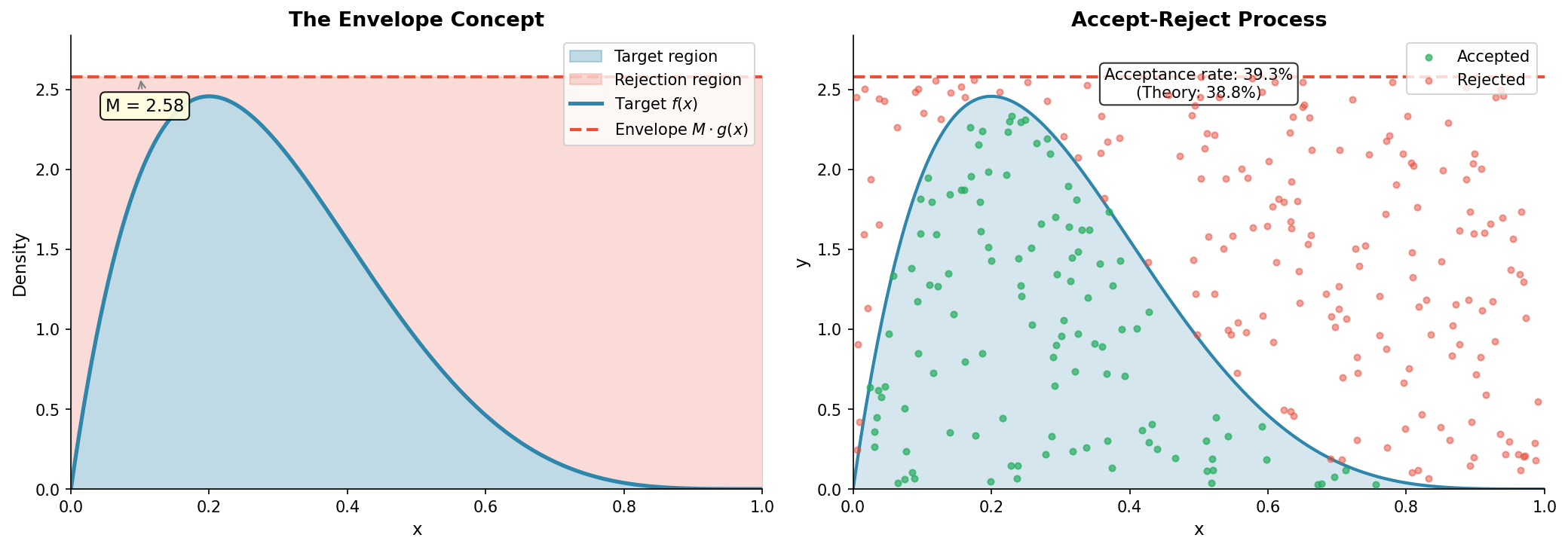
Target density f(x) enclosed by envelope Mg(x), with accepted region shaded — Fig. 65 **The Envelope Concept.** The target density \(f(x)\) (blue, shown here as a *normalized* density) is everywhere dominated by the envelope \(M \cdot g(x)\) (red dashed). Points uniformly distributed under the envelope will, when filtered to those under \(f(x)\), yield \(x\)-coordinates distributed according to \(f\). For this normalized case, the acceptance rate is \(1/M\).

Now here’s the key insight. We can easily generate points uniformly under \(M \cdot g(x)\):

Sample \(X \sim g(x)\) (a draw from the proposal distribution)
Sample \(Y \sim \text{Uniform}(0, M \cdot g(X))\) (a height uniformly distributed up to the envelope)

The pair \((X, Y)\) is uniformly distributed over the region under \(M \cdot g(x)\). If we now keep only those points with \(Y \le \tilde{f}(X)\)—those falling under the target density—the remaining points are uniformly distributed under \(\tilde{f}(x)\), and their \(x\)-coordinates follow \(\tilde{f}/C\).

The Accept-Reject Algorithm

We now formalize the geometric intuition into a precise algorithm.

Algorithm Statement

Given:

Target density \(\tilde{f}(x)\), possibly known only up to a normalizing constant
Proposal density \(g(x)\) from which we can sample directly
Envelope constant \(M\) such that \(\tilde{f}(x) \le M \cdot g(x)\) for all \(x\)

Algorithm (Accept-Reject Method)

To generate one sample from f(x) = tilde{f}(x) / C:

1. REPEAT:
   a. Draw X ~ g(x)                              [sample from proposal]
   b. Draw U ~ Uniform(0, 1)                     [independent uniform]
   c. Compute acceptance ratio:
      α(X) = tilde{f}(X) / [M · g(X)]
   d. IF U ≤ α(X):
      ACCEPT X and RETURN X
      ELSE:
      REJECT X and continue to next iteration

2. The returned X is an exact draw from f(x) = tilde{f}(x) / C

The key observation is that we don’t actually need to generate \(Y = U \cdot M \cdot g(X)\) explicitly. The condition \(Y \le \tilde{f}(X)\) is equivalent to \(U \cdot M \cdot g(X) \le \tilde{f}(X)\), which simplifies to \(U \le \tilde{f}(X) / [M \cdot g(X)] = \alpha(X)\).

Proof of Correctness

We now prove that accepted samples follow the target distribution \(f(x) = \tilde{f}(x)/C\).

Theorem (Correctness of Accept-Reject). Let \(\tilde{f}(x)\) be a non-negative measurable function with \(0 < C = \int \tilde{f}(x)\,dx < \infty\), and let \(g(x)\) be a probability density with \(g(x) > 0\) wherever \(\tilde{f}(x) > 0\). If \(\tilde{f}(x) \le M \cdot g(x)\) for all \(x\), then the accepted value \(X\) from the accept-reject algorithm has density \(f(x) = \tilde{f}(x)/C\).

Proof. Consider a single iteration. We generate \(X \sim g(x)\) and, independently, \(U \sim \text{Uniform}(0,1)\). We accept if \(U \le \tilde{f}(X)/[M \cdot g(X)]\).

For any measurable set \(A\), by independence of \(U\) and \(X\):

\[\begin{split}P(X \in A \text{ and accepted}) &= \int_A P\left(U \le \frac{\tilde{f}(x)}{M g(x)} \,\Big|\, X = x\right) g(x)\,dx \\ &= \int_A \frac{\tilde{f}(x)}{M g(x)} \cdot g(x)\,dx \\ &= \frac{1}{M} \int_A \tilde{f}(x)\,dx\end{split}\]

The overall probability of acceptance is:

\[P(\text{accepted}) = \frac{1}{M} \int_{-\infty}^{\infty} \tilde{f}(x)\,dx = \frac{C}{M}\]

By Bayes’ theorem:

\[P(X \in A \mid \text{accepted}) = \frac{P(X \in A \text{ and accepted})}{P(\text{accepted})} = \frac{\frac{1}{M}\int_A \tilde{f}(x)\,dx}{\frac{C}{M}} = \frac{\int_A \tilde{f}(x)\,dx}{C}\]

This is exactly the probability that a random variable with density \(f(x) = \tilde{f}(x)/C\) lies in \(A\). ∎

Key insight: The normalization constant \(C\) cancels in the acceptance ratio. We never need to compute \(\int \tilde{f}(x)\,dx\)—rejection sampling works even when \(\tilde{f}\) is known only up to proportionality.

Notation Convention

Throughout this section, we use:

\(\tilde{f}(x)\): unnormalized target (kernel), known up to proportionality
\(C = \int \tilde{f}(x)\,dx\): normalizing constant (often unknown)
\(f(x) = \tilde{f}(x)/C\): normalized density

The envelope condition is \(\tilde{f}(x) \le M \cdot g(x)\) for all \(x\). The algorithm uses only \(\tilde{f}\), never requiring \(C\).

Parameterization Convention

This section uses SciPy’s scale parameterization for the Gamma and Exponential distributions:

Gamma(shape, scale): \(f(x) = \frac{x^{\text{shape}-1} e^{-x/\text{scale}}}{\text{scale}^{\text{shape}} \Gamma(\text{shape})}\)
Exponential(scale): \(f(x) = \frac{1}{\text{scale}} e^{-x/\text{scale}}\)

The rate parameterization (common in statistics) relates via scale = 1/rate. When mathematical notation uses \(\text{Gamma}(\alpha, 1)\), the SciPy call is stats.gamma(a=alpha, scale=1).

Efficiency Analysis

Not every proposed sample is accepted. Understanding the acceptance rate is crucial for assessing computational cost.

Acceptance Probability: Two Cases

From the proof above, the acceptance probability depends on whether the target is normalized:

Acceptance Rate Summary

Case 1: Normalized target \(f(x)\) with \(\int f(x)\,dx = 1\):

\[P(\text{accept}) = \frac{1}{M}, \qquad \mathbb{E}[\text{iterations}] = M\]

Case 2: Unnormalized target \(\tilde{f}(x)\) with \(C = \int \tilde{f}(x)\,dx\):

\[P(\text{accept}) = \frac{C}{M}, \qquad \mathbb{E}[\text{iterations}] = \frac{M}{C}\]

Most textbook examples and library implementations assume Case 1 (normalized target). When working with unnormalized kernels—common in Bayesian inference—use Case 2.

Geometric interpretation: The acceptance probability equals the ratio of the area under \(\tilde{f}(x)\) (which is \(C\)) to the area under \(M \cdot g(x)\) (which is \(M\)). A tighter envelope (smaller \(M\)) means less wasted area and higher efficiency.

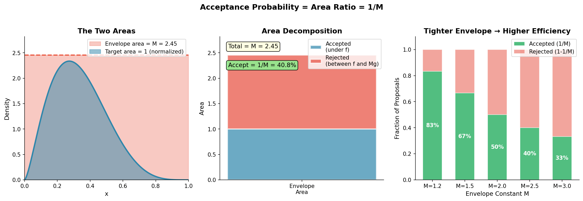
Three-panel visualization showing acceptance probability as area ratio — Fig. 66 **Acceptance Probability as Area Ratio.** This figure uses a *normalized* density \(f(x)\) (Case 1). Left: The target density \(f(x)\) (blue) sits inside the envelope \(M \cdot g(x)\) (red). Center: The envelope area decomposes into accepted (blue) and rejected (red) portions. Right: Smaller \(M\) values yield higher acceptance rates—a tighter envelope wastes less area. For normalized \(f\), the acceptance rate is \(1/M\).

The Optimal Envelope Constant

Given a proposal \(g(x)\), the smallest valid \(M\) is:

(13)\[M^* = \sup_x \frac{\tilde{f}(x)}{g(x)}\]

Using \(M^*\) maximizes acceptance probability. Any \(M > M^*\) is valid but wasteful; any \(M < M^*\) violates the envelope condition and produces incorrect samples.

Common Pitfall ⚠️

Using M that’s too small: If \(M \cdot g(x) < \tilde{f}(x)\) for some \(x\), samples from the region where the envelope dips below the target are underrepresented. This is a silent error—the algorithm runs but produces biased samples. Always verify that your envelope truly dominates the target, especially in tail regions.

Choosing the Proposal Distribution

The efficiency of rejection sampling hinges on choosing a proposal \(g(x)\) that closely approximates the target \(\tilde{f}(x)\) while remaining easy to sample.

Desiderata for Proposals

A good proposal distribution should satisfy:

Easy to sample: We need fast, direct sampling from \(g(x)\). Good choices include uniform, exponential, normal, Cauchy, and mixtures of these.
Support covers target: Wherever \(\tilde{f}(x) > 0\), we need \(g(x) > 0\). Otherwise, some regions of the target receive zero probability mass.
Shape matches target: Ideally, the ratio \(\tilde{f}(x)/g(x)\) should be nearly constant. Large variations in this ratio force \(M\) to be large, reducing efficiency.
Tail behavior matches or exceeds: If \(\tilde{f}(x)\) has heavy tails, \(g(x)\) must have at least as heavy tails. A light-tailed proposal for a heavy-tailed target leads to \(M = \infty\).

Finding the Envelope Constant

Given \(\tilde{f}\) and \(g\), we must compute \(M^* = \sup_x \tilde{f}(x)/g(x)\). Several approaches are available:

Analytical optimization: For well-behaved functions, calculus yields the maximum. Set the derivative of \(\tilde{f}(x)/g(x)\) to zero and solve.

Numerical optimization: Use scipy.optimize.minimize_scalar to find the maximum of \(\tilde{f}(x)/g(x)\).

Grid search: Evaluate the ratio on a fine grid covering the support, then take the maximum plus a small safety margin.

Bounding arguments: Sometimes theoretical bounds are available. For instance, if \(\tilde{f}\) is a product of terms each bounded by a constant, those bounds can be combined.

Example 💡 Finding M for Beta(2.5, 6) with Uniform Proposal

Setup (using normalized density): Target is \(f(x) = \frac{x^{1.5}(1-x)^5}{B(2.5, 6)}\) on \([0, 1]\), which is the normalized Beta(2.5, 6) density. Proposal is \(g(x) = 1\) (uniform on \([0, 1]\)).

Find M: For a uniform proposal with normalized target, \(M = \max_x f(x)\). The mode of Beta(\(\alpha, \beta\)) with \(\alpha, \beta > 1\) is \(x^* = (\alpha - 1)/(\alpha + \beta - 2)\).

Here \(x^* = 1.5/6.5 \approx 0.2308\). Computing the normalized density at the mode:

\[M^* = f(x^*) = \frac{(0.2308)^{1.5}(0.7692)^5}{B(2.5, 6)} \approx 2.61\]

Acceptance rate (Case 1, normalized): \(P(\text{accept}) = 1/M^* \approx 38.3\%\).

Alternative (unnormalized): If using the kernel \(\tilde{f}(x) = x^{1.5}(1-x)^5\) directly, then \(M^* = k(x^*) \approx 0.0297\) and \(C = B(2.5, 6) \approx 0.01137\), giving \(P(\text{accept}) = C/M^* \approx 38.3\%\)—the same result.

Numerical Approaches for Finding M

When analytical optimization is difficult, numerical methods provide \(M\):

Grid search: Evaluate \(\tilde{f}(x)/g(x)\) on a dense grid covering the support, then take the maximum with a safety margin:

def find_M_grid(target_pdf, proposal_pdf, x_min, x_max, n_grid=10000):
    """
    Find envelope constant M via grid search.

    Parameters
    ----------
    target_pdf : callable
        Target density or kernel (normalized or unnormalized).
    proposal_pdf : callable
        Proposal density (must be normalized).
    x_min, x_max : float
        Bounds for the support.
    n_grid : int
        Number of grid points.

    Returns
    -------
    float
        Envelope constant M with 2% safety margin.
    """
    x_grid = np.linspace(x_min, x_max, n_grid)

    # Vectorized evaluation
    g_vals = proposal_pdf(x_grid)
    f_vals = target_pdf(x_grid)

    # Avoid division by zero
    valid = g_vals > 1e-15
    ratios = np.zeros_like(x_grid)
    ratios[valid] = f_vals[valid] / g_vals[valid]

    M_grid = np.max(ratios)

    # Safety margin: 1-2% above grid maximum
    return M_grid * 1.02

Numerical optimization: Use scipy.optimize to find the maximum directly:

from scipy.optimize import minimize_scalar

def find_M_optimize(target_pdf, proposal_pdf, bounds):
    """Find M via numerical optimization."""

    def neg_ratio(x):
        g = proposal_pdf(x)
        if g < 1e-15:
            return 0  # Avoid division issues
        return -target_pdf(x) / g

    result = minimize_scalar(neg_ratio, bounds=bounds, method='bounded')
    M_optimal = -result.fun

    return M_optimal * 1.01  # Small safety margin

Adaptive refinement: For distributions with sharp peaks or boundary behavior, combine coarse grid search with local refinement near suspected maxima.

Common Pitfall ⚠️

Grid search misses boundary maxima: If \(\tilde{f}(x)/g(x)\) peaks at or near a boundary, a naive grid may miss it. Always include points very close to boundaries (e.g., \(x = 10^{-6}\) for distributions on \([0, \infty)\)), and verify that your computed \(M\) truly dominates by checking \(\tilde{f}(x) \le M \cdot g(x)\) at random test points.

Strategies for Proposal Selection

Choosing a good proposal is both art and science. The goal is to minimize \(M = \sup_x \tilde{f}(x)/g(x)\), which means matching the shape of the target—not just covering its support.

Principle 1: Support coverage is necessary but not sufficient

The proposal must satisfy \(g(x) > 0\) wherever \(\tilde{f}(x) > 0\). But merely covering the support can yield terrible efficiency. For Beta(0.5, 5) on \([0, 1]\), a Uniform(0, 1) proposal gives \(M \approx 5.7\) (17.5% acceptance), while a well-tuned Beta proposal achieves \(M \approx 1.3\) (77% acceptance).

The Fundamental Requirement

Rejection sampling requires:

\[\sup_x \frac{\tilde{f}(x)}{g(x)} < \infty\]

Equivalently, the ratio \(\tilde{f}/g\) must be bounded on the entire support. This single criterion unifies the tail behavior and singularity constraints discussed below.

Principle 2: Match tail behavior to avoid infinite M

If the target has heavier tails than the proposal, the ratio \(\tilde{f}(x)/g(x) \to \infty\) as \(|x| \to \infty\), making \(M = \infty\). This is a hard constraint:

Normal target → Normal, Cauchy, or Student-t proposal all work
Cauchy target → Normal proposal fails (\(M = \infty\))
Cauchy target → Cauchy or heavier-tailed proposal required

Principle 3: Match singularities for unbounded densities

If \(\tilde{f}(x) \to \infty\) at some point (e.g., Beta(0.5, 2) near \(x = 0\)), a bounded proposal cannot dominate. The proposal must have a matching or stronger singularity. See Exercise 2 for the Gamma(0.5, 1) case.

Principle 4: Shape matching minimizes M

The ideal proposal has \(g(x) \propto \tilde{f}(x)\), giving \(M = C\) (100% acceptance after normalization). In practice, we approximate this:

Table 20 Proposal Selection by Target Shape
Target Shape	Proposal Options	Efficiency Considerations
Symmetric, light-tailed (e.g., truncated normal)	Normal, scaled to match spread	Very efficient if variance matched; \(M \approx 1.1\text{-}1.5\)
Skewed on \([0, 1]\) (e.g., Beta(2, 8))	Beta with similar skew, or mixture of Betas	Uniform is simple but inefficient; Beta proposal can achieve \(M < 1.5\)
Skewed on \([0, \infty)\) (e.g., Gamma, Weibull)	Gamma or Exponential with rate matching mode	Match tail decay rate; heavier proposal tail is safer
Heavy-tailed (e.g., Cauchy, Pareto)	Cauchy, Student-t, or Pareto	Must use heavy-tailed proposal; normal fails
Multimodal	Mixture matching mode locations	Single unimodal proposal forces large \(M\); mixtures dramatically improve efficiency
Log-concave	Adaptive Rejection Sampling (ARS)	Envelope adapts during sampling; very efficient

Example: Beta(2, 8) — Comparing Proposals (Normalized Target)

from scipy import stats
import numpy as np

target = stats.beta(2, 8)  # Normalized density
x = np.linspace(0.001, 0.999, 10000)
f = target.pdf(x)

# Option 1: Uniform(0, 1) proposal
g_uniform = np.ones_like(x)
M_uniform = np.max(f / g_uniform)
# Case 1 (normalized): acceptance = 1/M
print(f"Uniform proposal: M = {M_uniform:.2f}, acceptance = {1/M_uniform:.1%}")

# Option 2: Beta(2, 7) proposal (similar shape)
proposal = stats.beta(2, 7)
g_beta = proposal.pdf(x)
M_beta = np.max(f / g_beta)
print(f"Beta(2,7) proposal: M = {M_beta:.2f}, acceptance = {1/M_beta:.1%}")

# Option 3: Beta(1.5, 6) proposal (slightly different)
proposal2 = stats.beta(1.5, 6)
g_beta2 = proposal2.pdf(x)
M_beta2 = np.max(f / g_beta2)
print(f"Beta(1.5,6) proposal: M = {M_beta2:.2f}, acceptance = {1/M_beta2:.1%}")

Output:

Uniform proposal: M = 2.62, acceptance = 38.2%
Beta(2,7) proposal: M = 1.18, acceptance = 84.7%
Beta(1.5,6) proposal: M = 1.31, acceptance = 76.3%

The Beta(2, 7) proposal—chosen to approximate the target’s shape—achieves more than double the acceptance rate of the uniform proposal.

Practical Guidance

Start simple: Uniform or normal proposals are easy to implement and debug. Use them first to verify correctness.
Profile before optimizing: If acceptance rate is above 20-30%, the simple proposal may be adequate. Optimize only if efficiency matters.
Use the same family when possible: For a Gamma target, try a Gamma proposal with slightly larger variance. For Beta targets, try Beta proposals.
Verify envelope condition: After choosing \(g\) and computing \(M\), always verify \(\tilde{f}(x) \le M \cdot g(x)\) at many points, especially near boundaries and modes.

Python Implementation

Let’s implement rejection sampling and apply it to several distributions.

Basic Implementation

import numpy as np
from scipy import stats

def rejection_sample(target_pdf, proposal_sampler, proposal_pdf, M,
                     n_samples, seed=None):
    """
    Generate samples from target using rejection sampling.

    Parameters
    ----------
    target_pdf : callable
        Function computing f(x) or tilde{f}(x).
    proposal_sampler : callable
        Function that returns one sample from g(x).
    proposal_pdf : callable
        Function computing g(x).
    M : float
        Envelope constant such that target_pdf(x) <= M * proposal_pdf(x).
    n_samples : int
        Number of samples to generate.
    seed : int, optional
        Random seed for reproducibility.

    Returns
    -------
    samples : ndarray
        Array of n_samples draws from the target distribution.
    acceptance_rate : float
        Fraction of proposals that were accepted.

    Notes
    -----
    If target_pdf is normalized, acceptance rate ≈ 1/M.
    If target_pdf is unnormalized with integral C, acceptance rate ≈ C/M.
    """
    rng = np.random.default_rng(seed)
    samples = []
    n_proposals = 0

    while len(samples) < n_samples:
        # Step 1: Draw from proposal
        x = proposal_sampler(rng)
        n_proposals += 1

        # Step 2: Draw uniform for acceptance test
        u = rng.random()

        # Step 3: Accept or reject
        acceptance_prob = target_pdf(x) / (M * proposal_pdf(x))

        if u <= acceptance_prob:
            samples.append(x)

    return np.array(samples), len(samples) / n_proposals

Example 💡 Sampling from Beta(2.5, 6) — Normalized Target (Case 1)

Given: Target is Beta(2.5, 6) using the normalized pdf from scipy; proposal is Uniform(0, 1)

Acceptance rate formula: Since we use normalized \(f\), acceptance rate is \(1/M\).

Implementation:

import numpy as np
from scipy import stats

# Target: Beta(2.5, 6) - NORMALIZED pdf via scipy
alpha, beta_param = 2.5, 6.0
target_dist = stats.beta(alpha, beta_param)
target_pdf = target_dist.pdf  # Normalized, vectorized

# Proposal: Uniform(0, 1)
def proposal_sampler(rng):
    return rng.random()

def proposal_pdf(x):
    return np.where((x >= 0) & (x <= 1), 1.0, 0.0)

# Find M: maximum of normalized Beta density
x_grid = np.linspace(0.001, 0.999, 10000)
M = target_pdf(x_grid).max() * 1.01  # 1% safety margin

print(f"Envelope constant M = {M:.4f}")
print(f"Expected acceptance rate (Case 1: 1/M) = {1/M:.1%}")

# Generate samples
samples, acc_rate = rejection_sample(
    target_pdf, proposal_sampler, proposal_pdf, M,
    n_samples=10000, seed=42
)

print(f"Actual acceptance rate = {acc_rate:.1%}")
print(f"Sample mean = {samples.mean():.4f} (theory: {alpha/(alpha+beta_param):.4f})")

Output:

Envelope constant M = 2.6360
Expected acceptance rate (Case 1: 1/M) = 37.9%
Actual acceptance rate = 38.2%
Sample mean = 0.2937 (theory: 0.2941)

The acceptance rate matches the theoretical \(1/M \approx 38\%\), confirming we’re in Case 1.

Example 💡 Sampling from Beta(2.5, 6) — Unnormalized Kernel (Case 2)

Given: Target is the unnormalized kernel \(\tilde{f}(x) = x^{1.5}(1-x)^5\); proposal is Uniform(0, 1)

Acceptance rate formula: Since we use unnormalized \(\tilde{f}\), acceptance rate is \(C/M\) where \(C = B(2.5, 6)\).

Implementation:

import numpy as np
from scipy import special

alpha, beta_param = 2.5, 6.0

# UNNORMALIZED kernel
def kernel(x):
    return x**(alpha-1) * (1-x)**(beta_param-1)

# Normalizing constant (often unknown in practice)
C = special.beta(alpha, beta_param)
print(f"Normalizing constant C = B({alpha}, {beta_param}) = {C:.6f}")

# Proposal: Uniform(0, 1)
def proposal_sampler(rng):
    return rng.random()

def proposal_pdf(x):
    return 1.0

# Find M for kernel
x_grid = np.linspace(0.001, 0.999, 10000)
M = kernel(x_grid).max() * 1.01

print(f"Envelope constant M = {M:.6f}")
print(f"Expected acceptance rate (Case 2: C/M) = {C/M:.1%}")

# Generate samples
samples, acc_rate = rejection_sample(
    kernel, proposal_sampler, proposal_pdf, M,
    n_samples=10000, seed=42
)

print(f"Actual acceptance rate = {acc_rate:.1%}")

Output:

Normalizing constant C = B(2.5, 6) = 0.011370
Envelope constant M = 0.030001
Expected acceptance rate (Case 2: C/M) = 37.9%
Actual acceptance rate = 38.2%

Key observation: Both approaches yield the same 38% acceptance rate—the normalized and unnormalized formulations are equivalent. Use Case 1 formula \(1/M\) when your pdf is normalized; use Case 2 formula \(C/M\) when working with kernels.

Vectorized Implementation for Speed

The basic implementation loops over individual samples. For better performance, we can generate batches of proposals and filter:

def rejection_sample_vectorized(target_pdf, proposal_sampler_batch,
                                proposal_pdf, M, n_samples, seed=None):
    """
    Vectorized rejection sampling for improved performance.

    Parameters
    ----------
    proposal_sampler_batch : callable
        Function that takes (rng, batch_size) and returns batch_size samples.

    Notes
    -----
    For normalized targets, acceptance rate ≈ 1/M.
    For unnormalized targets with integral C, acceptance rate ≈ C/M.
    """
    rng = np.random.default_rng(seed)
    samples = []
    n_proposals = 0

    # Estimate batch size based on expected acceptance rate
    batch_size = max(100, int(2 * M * n_samples / 10))

    while len(samples) < n_samples:
        # Generate batch of proposals
        x_batch = proposal_sampler_batch(rng, batch_size)
        u_batch = rng.random(batch_size)
        n_proposals += batch_size

        # Vectorized acceptance test
        f_vals = target_pdf(x_batch)
        g_vals = proposal_pdf(x_batch)
        acceptance_probs = f_vals / (M * g_vals)

        # Accept where u <= acceptance probability
        accepted = x_batch[u_batch <= acceptance_probs]
        samples.extend(accepted)

    return np.array(samples[:n_samples]), n_samples / n_proposals

Implementation Note

For true vectorization, target_pdf and proposal_pdf must accept array inputs and return arrays. SciPy’s stats.distribution.pdf methods support this natively. If your target is a custom function, use np.vectorize as a quick fix, though this provides no speed benefit over explicit loops. For performance-critical code, rewrite the PDF using NumPy array operations.

The Squeeze Principle

When the target density \(\tilde{f}(x)\) is expensive to evaluate, we can accelerate rejection sampling using a squeeze function (also called a lower envelope). The idea, introduced by Marsaglia [Marsaglia1977], is to construct a cheap-to-evaluate function \(\ell(x)\) satisfying:

\[0 \le \ell(x) \le \tilde{f}(x) \le M \cdot g(x) \quad \text{for all } x\]

The modified algorithm becomes:

To generate one sample from f(x) with squeeze:

1. REPEAT:
   a. Draw X ~ g(x)
   b. Draw U ~ Uniform(0, 1)
   c. IF U ≤ ℓ(X) / [M · g(X)]:
      ACCEPT X immediately (without evaluating tilde{f})
   d. ELSE IF U ≤ tilde{f}(X) / [M · g(X)]:
      ACCEPT X (requires evaluating tilde{f})
   e. ELSE:
      REJECT X

2. Return accepted X

The squeeze function acts as a “fast accept” gate. If the uniform variate falls below \(\ell(X)/[M \cdot g(X)]\), we accept without ever computing \(\tilde{f}(X)\). Only when \(U\) falls between the squeeze and the envelope do we need the expensive \(\tilde{f}\) evaluation.

Efficiency gain: If \(\ell(x)\) is close to \(\tilde{f}(x)\), most acceptances occur at step (c), avoiding the costly \(\tilde{f}(x)\) evaluation. This is particularly valuable when \(\tilde{f}\) involves special functions, numerical integration, or complex likelihood computations.

Valid Squeeze Construction

Critical requirement: The squeeze function must satisfy \(\ell(x) \le \tilde{f}(x)\) for ALL \(x\) in the support. A function that exceeds the target anywhere is not a valid squeeze and will produce biased fast-accepts.

Common Pitfall ⚠️

Invalid “tent” squeeze for unimodal densities: A piecewise linear “tent” in density space connecting \((0, 0)\), \((x^*, f(x^*))\), \((1, 0)\) (where \(x^*\) is the mode) is not a valid squeeze for most unimodal densities. For example, with Beta(5, 5):

The tent has area \(\frac{1}{2} \cdot 1 \cdot f(0.5) = \frac{1}{2} \cdot 2.46 = 1.23\)
But any valid squeeze must have area \(\le 1\) (since \(\int f = 1\))
The tent actually exceeds the Beta(5, 5) density on substantial interior intervals

An area exceeding 1 is a red flag that the construction is invalid.

Safe construction for log-concave targets: For log-concave densities (where \(\log \tilde{f}(x)\) is concave), a provably valid squeeze can be constructed using secant lines in log-space. Many important distributions are log-concave:

Normal: \(\log \phi(x) \propto -x^2/2\) (concave parabola)
Exponential: \(\log(\lambda e^{-\lambda x}) \propto -\lambda x\) (linear, hence concave)
Gamma with \(\alpha \ge 1\): \(\log f(x) \propto (\alpha-1)\log x - x\) (concave for \(\alpha \ge 1\))
Beta with \(\alpha, \beta \ge 1\): log-concave on \((0, 1)\)
Logistic, truncated log-normal

Log-space secant squeeze: Choose anchor points \(x_0 < x_1 < \cdots < x_K\) and define:

\[\underline{h}(x) = \text{piecewise-linear interpolation of } \log \tilde{f}(x_k)\]

By concavity of \(\log \tilde{f}\), the secant lines lie below the curve: \(\underline{h}(x) \le \log \tilde{f}(x)\). Exponentiating:

\[\ell(x) = \exp(\underline{h}(x)) \le \tilde{f}(x)\]

This construction is guaranteed valid for log-concave targets.

Example 💡 Valid Squeeze for Beta(5, 5) via Log-Space Secants

Beta(5, 5) is log-concave since \(\alpha, \beta \ge 1\). We construct a squeeze using linear interpolation in log-space:

import numpy as np
from scipy import stats

target = stats.beta(5, 5)

# Anchor points
x_anchors = np.array([0.1, 0.3, 0.5, 0.7, 0.9])
log_f_anchors = np.log(target.pdf(x_anchors))

def log_squeeze(x):
    """Piecewise linear interpolation in log-space."""
    return np.interp(x, x_anchors, log_f_anchors)

def squeeze(x):
    """Valid squeeze: exp of log-space interpolation."""
    return np.exp(log_squeeze(x))

# Verify squeeze validity
x_test = np.linspace(0.01, 0.99, 10000)
f_vals = target.pdf(x_test)
squeeze_vals = squeeze(x_test)

violations = np.sum(squeeze_vals > f_vals * 1.0001)  # Allow tiny numerical error
print(f"Violations: {violations} (should be 0)")

# Squeeze efficiency
squeeze_area = np.trapz(squeeze_vals, x_test)
print(f"Squeeze area: {squeeze_area:.4f} (must be ≤ 1)")
print(f"Fast-accept fraction: ~{squeeze_area:.1%}")

Output:

Violations: 0 (should be 0)
Squeeze area: 0.8712 (must be ≤ 1)
Fast-accept fraction: ~87.1%

The log-space construction is valid (no violations) and achieves ~87% fast-accepts, avoiding expensive Beta function evaluations for most proposals.

Example 💡 Squeeze for Normal Density

From the Taylor expansion \(e^{-x^2/2} \ge 1 - x^2/2\) for \(|x| \le \sqrt{2}\), we can use \(\ell(x) = (1 - x^2/2)/\sqrt{2\pi}\) as a squeeze function for the standard normal density within \([-\sqrt{2}, \sqrt{2}]\). This avoids the exponential evaluation for about 61% of proposals when using a Cauchy envelope.

Geometric Example: Sampling from the Unit Disk

A classic application of rejection sampling is generating points uniformly distributed in a geometric region. Consider sampling uniformly from the unit disk \(\{(x, y) : x^2 + y^2 \le 1\}\).

Target: Uniform distribution on the disk (density \(f(x,y) = 1/\pi\) inside, 0 outside)

Proposal: Uniform on the bounding square \([-1, 1]^2\) (density \(g(x,y) = 1/4\))

Envelope constant: Inside the disk, \(f(x,y)/g(x,y) = (1/\pi)/(1/4) = 4/\pi\), so \(M = 4/\pi \approx 1.273\).

Acceptance rate (Case 1, normalized): \(1/M = \pi/4 \approx 78.5\%\), which equals the ratio of areas (disk area \(\pi\) divided by square area 4).

import numpy as np

def sample_unit_disk(n_samples, seed=None):
    """
    Sample uniformly from the unit disk via rejection.

    Uses normalized densities, so acceptance rate = 1/M = π/4 ≈ 78.5%.
    """
    rng = np.random.default_rng(seed)
    samples = []
    n_proposals = 0

    while len(samples) < n_samples:
        # Propose from uniform square [-1, 1]²
        x = rng.uniform(-1, 1)
        y = rng.uniform(-1, 1)
        n_proposals += 1

        # Accept if inside disk
        if x*x + y*y <= 1:
            samples.append((x, y))

    return np.array(samples), n_samples / n_proposals

# Generate 10,000 points
points, acc_rate = sample_unit_disk(10000, seed=42)
print(f"Acceptance rate: {acc_rate:.3f} (theory: π/4 = {np.pi/4:.3f})")
print(f"Points shape: {points.shape}")

Output:

Acceptance rate: 0.785 (theory: π/4 = 0.785)
Points shape: (10000, 2)

This “hit-and-miss” approach generalizes to any region where membership can be tested: sample from a bounding box and reject points outside the target region. The efficiency depends on how well the bounding box fits the region.

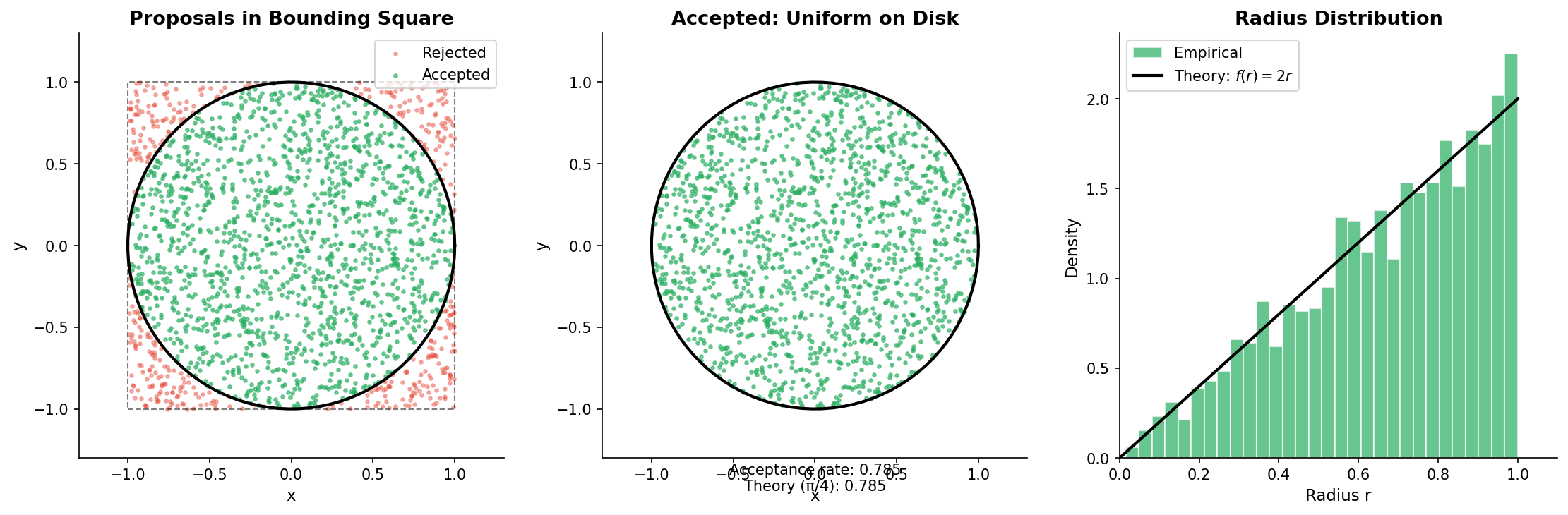
Rejection sampling for uniform disk: accepted points inside circle, rejected in corners — Fig. 67 **Rejection Sampling for the Unit Disk (Normalized Densities).** Blue points are accepted (inside disk); red points are rejected (in square corners). Using normalized densities \(f = 1/\pi\) and \(g = 1/4\), the acceptance rate is \(1/M = \pi/4 \approx 78.5\%\).

Worked Examples

We now apply rejection sampling to several important scenarios, explicitly noting whether we use normalized or unnormalized targets.

Example 1: Truncated Normal Distribution

A truncated normal distribution restricts the standard normal to an interval \([a, b]\). When \([a, b]\) lies in the tails, inversion methods become numerically unstable, but rejection sampling offers a simple solution.

Target (unnormalized kernel): \(\tilde{f}(x) = \phi(x) \cdot \mathbf{1}\{a \le x \le b\}\)

Normalizing constant: \(C = \Phi(b) - \Phi(a)\)

Proposal: The untruncated normal \(g(x) = \phi(x)\)

Envelope: Since \(\tilde{f}(x) = \phi(x)\) when \(x \in [a, b]\) and 0 otherwise, we have \(\tilde{f}(x) \le g(x)\), so \(M = 1\).

Acceptance rate (Case 2, unnormalized): \(P(\text{accept}) = C/M = \Phi(b) - \Phi(a)\).

Acceptance criterion: Accept \(X \sim \mathcal{N}(0, 1)\) if \(a \le X \le b\).

def truncated_normal(a, b, n_samples, seed=None):
    """
    Sample from N(0,1) truncated to [a, b] via rejection.

    Using unnormalized kernel, so acceptance rate = C/M = Φ(b) - Φ(a).
    """
    rng = np.random.default_rng(seed)
    samples = []
    n_proposals = 0

    while len(samples) < n_samples:
        x = rng.standard_normal()
        n_proposals += 1
        if a <= x <= b:
            samples.append(x)

    # C = Φ(b) - Φ(a), M = 1, so P(accept) = C/M = C
    theoretical_rate = stats.norm.cdf(b) - stats.norm.cdf(a)
    actual_rate = len(samples) / n_proposals

    return np.array(samples), actual_rate, theoretical_rate

# Example: truncate to [1, 3] (right tail)
samples, actual, theory = truncated_normal(1, 3, 10000, seed=42)
print(f"Truncated N(0,1) to [1, 3]:")
print(f"  Theoretical acceptance rate (C/M): {theory:.3%}")
print(f"  Actual acceptance rate: {actual:.3%}")
print(f"  Sample mean: {samples.mean():.4f}")

Output:

Truncated N(0,1) to [1, 3]:
  Theoretical acceptance rate (C/M): 15.7%
  Actual acceptance rate: 15.8%
  Sample mean: 1.5239

Common Pitfall ⚠️

Extreme truncation: If \([a, b]\) lies far in the tail (e.g., \([4, 6]\)), the acceptance rate becomes tiny: \(\Phi(6) - \Phi(4) \approx 0.003\%\). For extreme truncation, use specialized algorithms like Robert’s exponential tilting method or inverse CDF with careful numerical handling.

Example 2: Gamma Distribution

The Gamma distribution with non-integer shape parameter has no simple transformation from uniforms. Rejection sampling provides an efficient solution.

Target: \(\text{Gamma}(\alpha, 1)\) with \(\alpha > 0\)

For \(\alpha \ge 1\), Ahrens-Dieter and other algorithms use rejection with carefully chosen envelopes. Here’s a simplified version using an exponential proposal for \(\alpha \ge 1\):

def gamma_rejection(alpha, n_samples, seed=None):
    """
    Sample Gamma(alpha, 1) using rejection with exponential envelope.

    Uses normalized densities throughout.
    """
    if alpha < 1:
        # Use transformation: Gamma(alpha) = Gamma(alpha+1) * U^(1/alpha)
        samples = gamma_rejection(alpha + 1, n_samples, seed)
        rng = np.random.default_rng(seed)
        u = rng.random(n_samples)
        return samples * u**(1/alpha)

    rng = np.random.default_rng(seed)

    # For alpha >= 1, use exponential(1/alpha) as proposal
    rate = 1 / alpha
    mode = alpha - 1

    # M = f(mode) / g(mode) where both are normalized
    f_mode = mode**(alpha - 1) * np.exp(-mode) / np.math.gamma(alpha)
    g_mode = rate * np.exp(-rate * mode)
    M = f_mode / g_mode * 1.01  # safety margin

    samples = []
    n_proposals = 0

    while len(samples) < n_samples:
        x = rng.exponential(1 / rate)  # Exp(rate) sample
        u = rng.random()
        n_proposals += 1

        # Both pdfs normalized
        f_x = x**(alpha - 1) * np.exp(-x) / np.math.gamma(alpha)
        g_x = rate * np.exp(-rate * x)

        if u <= f_x / (M * g_x):
            samples.append(x)

    # Case 1 (normalized): acceptance = 1/M
    print(f"Gamma({alpha}): acceptance rate = {len(samples)/n_proposals:.1%} (theory: 1/M = {1/M:.1%})")
    return np.array(samples)

# Test
samples = gamma_rejection(2.5, 10000, seed=42)
print(f"Sample mean: {samples.mean():.3f} (theory: 2.5)")
print(f"Sample var:  {samples.var():.3f} (theory: 2.5)")

Example 3: Custom Posterior Distribution (Unnormalized)

Rejection sampling shines in Bayesian inference where posteriors are known only up to proportionality.

Scenario: Binomial likelihood with Beta prior yields Beta posterior, but suppose we want to apply rejection sampling without recognizing the conjugate form.

def bayesian_posterior_rejection(n_successes, n_trials, prior_alpha, prior_beta,
                                 n_samples, seed=None):
    """
    Sample from posterior of Binomial parameter θ using UNNORMALIZED kernel.

    Prior: θ ~ Beta(prior_alpha, prior_beta)
    Likelihood: X | θ ~ Binomial(n_trials, θ)
    Posterior kernel: tilde{f}(θ) ∝ θ^(α + x - 1) (1-θ)^(β + n - x - 1)

    Since kernel is unnormalized, acceptance rate = C/M.
    """
    # Posterior kernel (unnormalized)
    def posterior_kernel(theta):
        if theta <= 0 or theta >= 1:
            return 0.0
        return (theta**(prior_alpha + n_successes - 1) *
                (1 - theta)**(prior_beta + n_trials - n_successes - 1))

    # Use uniform proposal on [0, 1]
    x_grid = np.linspace(0.001, 0.999, 1000)
    kernel_vals = [posterior_kernel(x) for x in x_grid]
    M = max(kernel_vals) * 1.01

    # True posterior is Beta(α + x, β + n - x)
    post_alpha = prior_alpha + n_successes
    post_beta = prior_beta + n_trials - n_successes
    C = special.beta(post_alpha, post_beta)  # Normalizing constant

    rng = np.random.default_rng(seed)
    samples = []
    n_proposals = 0

    while len(samples) < n_samples:
        theta = rng.random()  # Uniform(0, 1)
        u = rng.random()
        n_proposals += 1

        if u <= posterior_kernel(theta) / M:
            samples.append(theta)

    actual_rate = n_samples / n_proposals
    theoretical_rate = C / M  # Case 2: unnormalized

    print(f"Acceptance rate: actual = {actual_rate:.1%}, theory (C/M) = {theoretical_rate:.1%}")

    return np.array(samples), actual_rate

# Example: 7 successes in 10 trials, uniform prior
from scipy import special
samples, acc_rate = bayesian_posterior_rejection(
    n_successes=7, n_trials=10,
    prior_alpha=1, prior_beta=1,  # uniform prior
    n_samples=10000, seed=42
)

# True posterior is Beta(8, 4)
print(f"Posterior mean: {samples.mean():.4f} (theory: {8/12:.4f})")

Limitations and the Curse of Dimensionality

Rejection sampling is elegant and exact, but it has fundamental limitations.

The High-Dimensional Problem

In \(d\) dimensions, the envelope condition becomes:

\[\tilde{f}(\mathbf{x}) \le M \cdot g(\mathbf{x}) \quad \text{for all } \mathbf{x} \in \mathbb{R}^d\]

The acceptance probability is still \(C/M\) (or \(1/M\) for normalized targets), but now \(M\) often grows exponentially with dimension.

Example: Target is \(\mathcal{N}(\mathbf{0}, \mathbf{I}_d)\) and proposal is \(\mathcal{N}(\mathbf{0}, \sigma^2 \mathbf{I}_d)\) with \(\sigma > 1\). The ratio \(f(\mathbf{x})/g(\mathbf{x})\) involves:

\[\frac{f(\mathbf{x})}{g(\mathbf{x})} = \sigma^d \exp\left[-\frac{\|\mathbf{x}\|^2}{2}\left(1 - \frac{1}{\sigma^2}\right)\right]\]

The maximum occurs at \(\mathbf{x} = \mathbf{0}\), giving \(M = \sigma^d\). For \(\sigma = 1.5\) and \(d = 20\), this is \(1.5^{20} \approx 3,300\)—a 0.03% acceptance rate!

Rule of thumb: Rejection sampling is usually practical for \(d \le 5\), sometimes up to \(d \approx 10\) with carefully matched proposals and mixtures, and rarely beyond.

When Rejection Sampling Fails

Rejection sampling becomes impractical when:

High dimensions: The curse of dimensionality makes finding a tight envelope nearly impossible.
Multimodal targets: A single proposal struggles to cover well-separated modes without huge \(M\).
Heavy tails with light-tailed proposals: If \(\tilde{f}(x)/g(x) \to \infty\) as \(|x| \to \infty\), no finite \(M\) exists.
Unknown mode location: Without knowing where the target is concentrated, any proposal is a guess.

Mixture proposals for multimodal targets: When the target has \(K\) well-separated modes, use a mixture proposal \(g(x) = \sum_{k=1}^K w_k g_k(x)\) where each component \(g_k\) covers one mode. Compute \(M = \sup_x \tilde{f}(x)/g(x)\) numerically. If each component \(g_k\) dominates the target in its region with constant \(M_k\), a practical (though conservative) bound is \(M \le \sum_k M_k\). This approach dramatically improves efficiency compared to a single broad proposal.

Practical guideline: Rejection sampling works well for \(d \le 5\) or so. For higher dimensions, consider Markov Chain Monte Carlo (Metropolis-Hastings, Gibbs sampling) which we develop in later chapters.

Connections to Other Methods

Rejection sampling is the ancestor of several more sophisticated techniques.

Importance Sampling

Where rejection sampling discards proposals that don’t pass the acceptance test, importance sampling keeps all proposals but assigns them weights:

\[w(x) = \frac{\tilde{f}(x)}{g(x)}\]

Expectations are then computed as weighted averages. Importance sampling avoids discarding samples but requires careful handling of weight variability. We develop this in detail in ch2.6-variance-reduction.

Markov Chain Monte Carlo

The Metropolis-Hastings algorithm generalizes rejection sampling to create a Markov chain whose stationary distribution is the target. Instead of independent proposals, it uses sequential proposals from a transition kernel. Rejected proposals don’t disappear—the chain stays at its current position. This modification allows MCMC to work efficiently in high dimensions where direct rejection sampling fails. See Chapter 5 for full development.

Adaptive Rejection Sampling

For log-concave densities (densities \(\tilde{f}(x)\) where \(\log \tilde{f}(x)\) is concave), the ARS algorithm [GilksWild1992] constructs an envelope adaptively during sampling. The key insight is that tangent lines to a concave function lie above the function, while secant lines lie below.

Log-concave examples: Many important distributions are log-concave:

Normal: \(\log \phi(x) \propto -x^2/2\) (concave parabola)
Exponential: \(\log(\lambda e^{-\lambda x}) \propto -\lambda x\) (linear, hence concave)
Gamma with \(\alpha \ge 1\): \(\log f(x) \propto (\alpha-1)\log x - x\) (concave for \(\alpha \ge 1\))
Beta with \(\alpha, \beta \ge 1\): log-concave on \((0, 1)\)
Logistic, log-normal truncated appropriately

The ARS algorithm:

Initialize with a few points \(S_n = \{x_0, x_1, \ldots, x_n\}\) where \(\log \tilde{f}(x_i)\) is known.
Construct upper envelope \(\bar{h}_n(x)\): piecewise linear, connecting tangent lines at \(x_i\). By concavity, this lies above \(\log \tilde{f}(x)\).
Construct lower envelope \(\underline{h}_n(x)\): piecewise linear through \((x_i, \log \tilde{f}(x_i))\). By concavity, this lies below \(\log \tilde{f}(x)\).
Sample from \(g_n(x) \propto \exp(\bar{h}_n(x))\) (piecewise exponential, easy to sample).
Squeeze test: If \(U \le \exp(\underline{h}_n(X) - \bar{h}_n(X))\), accept immediately.
Full test: Otherwise, evaluate \(\tilde{f}(X)\) and accept if \(U \le \tilde{f}(X)/g_n(X)\).
Adapt: If rejected (or if \(\tilde{f}(X)\) was evaluated), add \(X\) to \(S_n\), tightening future envelopes.

The adaptive nature means efficiency improves as sampling progresses—early rejections contribute information that speeds later sampling. ARS is particularly valuable within Gibbs samplers where full conditionals are often log-concave.

Limitation: ARS requires log-concavity. For non-log-concave targets (e.g., mixture distributions, heavy-tailed posteriors), the algorithm fails. The ARMS extension [GilksEtAl1995] handles non-log-concave targets by adding a Metropolis-Hastings correction step.

Practical Considerations

Numerical Stability

Several numerical issues can arise:

Underflow in density ratios: When \(\tilde{f}(x)\) is very small, \(\tilde{f}(x)/[M \cdot g(x)]\) may underflow to zero. Work with log-densities: accept if \(\log U \le \log \tilde{f}(x) - \log M - \log g(x)\).
Overflow in unnormalized densities: Large exponents can overflow. Again, log-densities help.
Zero proposal density: If \(g(x) = 0\) at a point where \(\tilde{f}(x) > 0\), the ratio is undefined. Ensure proposal support covers target support.

Log-space implementation for numerical stability:

def rejection_sample_log(log_target, log_proposal, proposal_sampler,
                         log_M, n_samples, seed=None):
    """
    Rejection sampling using log-densities for numerical stability.

    Accept if log(U) <= log_target(x) - log_M - log_proposal(x)

    Works for both normalized and unnormalized log_target.
    """
    rng = np.random.default_rng(seed)
    samples = []

    while len(samples) < n_samples:
        x = proposal_sampler(rng)
        log_u = np.log(rng.random())  # log(U) where U ~ Uniform(0,1)

        log_accept_prob = log_target(x) - log_M - log_proposal(x)

        if log_u <= log_accept_prob:
            samples.append(x)

    return np.array(samples)

This approach handles densities that would otherwise cause overflow or underflow in direct computation.

Verifying Correctness

Always verify your rejection sampler:

Check acceptance rate: Compare actual rate to theoretical \(1/M\) (normalized) or \(C/M\) (unnormalized).
Compare moments: Sample mean and variance should match theoretical values.
Visual comparison: Histogram of samples should match theoretical density.
Kolmogorov-Smirnov test: Statistical test for distribution match.

def verify_rejection_sampler(samples, true_dist, name="", is_normalized=True, M=None, C=None):
    """
    Verify rejection samples against known distribution.

    Parameters
    ----------
    is_normalized : bool
        If True, expected rate is 1/M. If False, expected rate is C/M.
    """
    print(f"{name} verification:")
    print(f"  Sample mean: {samples.mean():.4f}, Theory: {true_dist.mean():.4f}")
    print(f"  Sample std:  {samples.std():.4f}, Theory: {true_dist.std():.4f}")

    # KS test
    ks_stat, p_value = stats.kstest(samples, true_dist.cdf)
    print(f"  KS statistic: {ks_stat:.4f}, p-value: {p_value:.4f}")

    if p_value < 0.01:
        print("  WARNING: KS test suggests samples may not match target!")

Production Diagnostics

For production use, a sampler with built-in monitoring helps detect issues:

class RejectionSamplerWithDiagnostics:
    """Rejection sampler with performance monitoring."""

    def __init__(self, target_pdf, proposal_sampler, proposal_pdf, M,
                 is_normalized=True, C=None):
        """
        Parameters
        ----------
        is_normalized : bool
            If True, expect acceptance = 1/M. If False, expect C/M.
        C : float, optional
            Normalizing constant (required if is_normalized=False).
        """
        self.target_pdf = target_pdf
        self.proposal_sampler = proposal_sampler
        self.proposal_pdf = proposal_pdf
        self.M = M
        self.is_normalized = is_normalized
        self.C = C if C is not None else 1.0

        # Diagnostics
        self.n_proposed = 0
        self.n_accepted = 0
        self.acceptance_history = []

    def sample(self, size, batch_size=100, seed=None):
        """Sample with batch monitoring."""
        rng = np.random.default_rng(seed)
        samples = []

        while len(samples) < size:
            batch_accepted = 0

            for _ in range(min(batch_size, size - len(samples) + 100)):
                y = self.proposal_sampler(rng)
                self.n_proposed += 1

                u = rng.random()
                accept_prob = self.target_pdf(y) / (self.M * self.proposal_pdf(y))

                if u <= accept_prob:
                    samples.append(y)
                    self.n_accepted += 1
                    batch_accepted += 1

                    if len(samples) >= size:
                        break

            # Record batch acceptance rate
            if batch_size > 0:
                self.acceptance_history.append(batch_accepted / batch_size)

        return np.array(samples[:size])

    def get_diagnostics(self):
        """Return sampling diagnostics."""
        actual_rate = self.n_accepted / self.n_proposed if self.n_proposed > 0 else 0
        if self.is_normalized:
            theoretical_rate = 1 / self.M
        else:
            theoretical_rate = self.C / self.M

        return {
            'n_proposed': self.n_proposed,
            'n_accepted': self.n_accepted,
            'actual_acceptance_rate': actual_rate,
            'theoretical_rate': theoretical_rate,
            'efficiency': actual_rate / theoretical_rate,  # Should be ≈ 1
            'acceptance_history': self.acceptance_history,
            'case': 'normalized (1/M)' if self.is_normalized else f'unnormalized (C/M, C={self.C:.4f})'
        }

The efficiency metric should be close to 1.0; significant deviations indicate either an incorrect \(M\) or implementation bugs.

Chapter 2.5 Exercises: Rejection Sampling Mastery

These exercises build your understanding of rejection sampling from geometric intuition through practical implementation to recognizing its limitations. Each exercise connects the theoretical foundation to computational practice.

A Note on These Exercises

These exercises are designed to deepen your understanding of rejection sampling through hands-on exploration:

Exercise 1 verifies the fundamental theorem of simulation—that points under a curve have marginals following that density
Exercise 2 explores envelope constant computation, sensitivity, and the consequences of getting M wrong
Exercise 3 compares proposal distributions and develops intuition for efficient proposal selection
Exercise 4 implements the squeeze principle to accelerate sampling with expensive target evaluations
Exercise 5 demonstrates the curse of dimensionality through direct experimentation
Exercise 6 applies rejection sampling to Bayesian inference with unnormalized posteriors

Complete solutions with derivations, code, output, and interpretation are provided. Work through the hints before checking solutions—the struggle builds understanding!

Exercise 1: The Fundamental Theorem of Simulation

The theoretical foundation of rejection sampling rests on a beautiful geometric fact: if points \((X, U)\) are uniformly distributed over the region under a density curve \(f(x)\), then \(X\) has density \(f(x)\). This exercise verifies this principle empirically.

Background: Points Under a Curve

For any density \(f(x)\), the identity \(f(x) = \int_0^{f(x)} du\) implies that uniform samples from the set \(\{(x,u): 0 < u < f(x)\}\) have \(x\)-marginals distributed as \(f\). This observation transforms the abstract problem of sampling from \(f\) into the geometric problem of sampling uniformly from a region.

Direct verification for Exponential(1): Generate 100,000 points uniformly distributed in the region under the Exponential(1) density \(f(x) = e^{-x}\) for \(x \geq 0\). Extract the \(x\)-coordinates and verify they follow Exponential(1) using:
- Sample mean and variance (theory: both equal 1)
- K-S test against Exponential(1)
Hint: Sampling Under the Curve

Use rejection from a bounding box. For Exponential(1), the maximum density is \(f(0) = 1\). Sample \(X \sim \text{Uniform}(0, x_{\max})\) and \(U \sim \text{Uniform}(0, 1)\), accepting when \(U < e^{-X}\). Choose \(x_{\max}\) large enough to capture most of the mass (e.g., \(x_{\max} = 10\)).
Verify for Beta(2, 5): Repeat for Beta(2, 5) on \([0, 1]\). Sample uniformly from the region under the density and verify the \(x\)-marginals match the theoretical distribution.
Visualize the geometry: Create a scatter plot of 5,000 accepted \((x, u)\) pairs for Beta(2, 5), overlaid with the density curve. Explain why the point density varies across the plot.
Unnormalized case: The theorem works for unnormalized kernels too. Generate points under \(\tilde{f}(x) = x^2 e^{-x}\) (unnormalized Gamma(3,1) kernel) and verify the \(x\)-marginals follow Gamma(3, 1).

Exercise 2: Envelope Constant Sensitivity and Verification

The envelope constant \(M\) is crucial for rejection sampling correctness and efficiency. This exercise explores how to compute, verify, and understand the consequences of incorrect \(M\) values.

Background: The Critical Role of M

The envelope condition \(f(x) \leq M \cdot g(x)\) must hold for ALL \(x\) in the support. Using \(M\) too large wastes computation (low acceptance rate); using \(M\) too small produces biased samples (some regions underrepresented). The optimal \(M^* = \sup_x f(x)/g(x)\) achieves maximum efficiency while maintaining correctness.

Compute M analytically: For target Beta(3, 2) and proposal Uniform(0, 1):
- Find the mode of Beta(3, 2) and compute \(M^* = \max_x f(x)/g(x)\)
- Verify using numerical optimization
Verify the envelope condition: Generate a fine grid of points and check that \(f(x) \leq M \cdot g(x)\) everywhere. Plot \(f(x)\) and \(M \cdot g(x)\) together.
What happens with M too small?: Set \(M = 0.8 \cdot M^*\) (deliberately violating the envelope condition). Generate samples and compare:
- Sample mean vs theoretical mean
- K-S test (should fail!)
- Which regions are undersampled?
What happens with M too large?: Set \(M = 2 \cdot M^*\). Verify correctness (K-S test should pass) but measure efficiency loss.

Exercise 3: Proposal Distribution Comparison

The choice of proposal distribution dramatically affects rejection sampling efficiency. This exercise compares proposals for a challenging target: the Beta(0.5, 0.5) distribution (the arcsine distribution).

Background: The Arcsine Distribution

Beta(0.5, 0.5) has density \(f(x) = \frac{1}{\pi\sqrt{x(1-x)}}\) on \((0, 1)\). This U-shaped distribution is unbounded at both endpoints, making it challenging to envelope. The density diverges as \(x \to 0\) or \(x \to 1\), requiring proposals that also diverge at the boundaries.

Why Uniform fails: Show that using Uniform(0, 1) as proposal requires \(M = \infty\) (the envelope constant is unbounded).

Hint: Behavior at Boundaries

Compute \(\lim_{x \to 0^+} f(x)/g(x)\) where \(g(x) = 1\).
Beta proposal with matching singularities: Show that Beta(0.5, 0.5) as its own proposal gives \(M = 1\) (100% acceptance). This is trivial but illustrates the ideal.
Alternative proposal: Use Beta(0.3, 0.3) as a proposal (heavier singularities). Compute \(M^*\) numerically, implement rejection sampling, and report the acceptance rate.
Mixture proposal: Design a mixture of three Beta distributions to improve efficiency. Compare acceptance rates across all approaches.

Exercise 4: The Squeeze Principle

When the target density \(f(x)\) is expensive to evaluate, the squeeze principle can dramatically reduce computation by avoiding unnecessary evaluations.

Background: Fast Accept, Expensive Verify

The squeeze function \(\ell(x) \leq f(x)\) enables a two-stage acceptance test: if \(U \leq \ell(X)/[M \cdot g(X)]\), accept immediately without evaluating \(f\). Only when \(U\) falls between the squeeze and envelope do we need the costly \(f(X)\) evaluation. This is valuable when \(f\) involves special functions, numerical integration, or likelihood computations.

Design a squeeze for Beta(5, 5): The Beta(5, 5) density involves the Beta function \(B(5,5)\). Design a simple polynomial squeeze \(\ell(x)\) that lies below \(f(x)\) everywhere on \([0, 1]\).

Hint: Linear Squeeze

A piecewise linear function connecting \((0, 0)\), \((0.5, f(0.5))\), and \((1, 0)\) lies below the symmetric Beta(5,5) density.
Implement rejection with squeeze: Implement the two-stage algorithm. Track how often the squeeze test succeeds (fast accept) vs. how often full \(f(x)\) evaluation is needed.
Measure speedup: Compare wall-clock time with and without the squeeze, artificially making the target “expensive” by adding a delay.
Optimal squeeze design: For log-concave densities, secant lines provide a tighter squeeze. Implement this for Beta(5, 5) and compare squeeze efficiency.

Exercise 5: The Curse of Dimensionality

Rejection sampling’s acceptance rate degrades exponentially with dimension. This exercise demonstrates this fundamental limitation through direct experimentation.

Background: Exponential Degradation

When target and proposal are both \(d\)-dimensional distributions, the envelope constant typically scales as \(M = O(c^d)\) for some \(c > 1\). With acceptance rate \(1/M\), the expected proposals per sample grows exponentially: \(\mathbb{E}[\text{proposals}] = c^d\). This makes rejection sampling impractical for \(d \gtrsim 5\).

Theoretical analysis: For target \(\mathcal{N}(\mathbf{0}, \mathbf{I}_d)\) and proposal \(\mathcal{N}(\mathbf{0}, \sigma^2\mathbf{I}_d)\) with \(\sigma > 1\), derive \(M = \sigma^d\) and the acceptance rate \(\sigma^{-d}\).
Empirical verification: Implement rejection sampling for \(d = 1, 2, 3, 5, 10\) with \(\sigma = 1.5\). Measure actual acceptance rates and compare to theory.
Practical limits: For each dimension, estimate how many proposals are needed to generate 1,000 samples. At what dimension does this become impractical (e.g., > 1 million proposals)?
Visualize the degradation: Plot acceptance rate vs. dimension on a log scale. Fit an exponential decay model.

Exercise 6: Bayesian Posterior Sampling

Rejection sampling is particularly valuable for Bayesian inference, where posteriors are known only up to a normalizing constant. This exercise applies rejection sampling to a non-conjugate posterior.

Background: Posteriors Without Conjugacy

For conjugate prior-likelihood pairs (like Beta-Binomial), the posterior has a known form. But many real problems lack conjugacy. Rejection sampling provides exact posterior samples when we can evaluate the unnormalized posterior \(p(\theta|x) \propto p(x|\theta)p(\theta)\) and find a suitable envelope.

Non-conjugate setup: Consider a Poisson likelihood with a log-normal prior on the rate parameter \(\lambda\):
- Data: \(x_1, \ldots, x_n \sim \text{Poisson}(\lambda)\)
- Prior: \(\lambda \sim \text{LogNormal}(\mu_0, \sigma_0^2)\)
Write the unnormalized posterior \(p(\lambda|x) \propto p(x|\lambda)p(\lambda)\).
Design a proposal: The posterior is unimodal and concentrated. Use a Gamma distribution as a proposal, choosing parameters to roughly match the posterior’s mode and spread. Find \(M\) numerically.
Implement and verify: Generate 10,000 posterior samples. Compute the posterior mean, median, and 95% credible interval for \(\lambda\).
Compare to conjugate approximation: If we had used a Gamma prior instead of log-normal, we could compute the posterior analytically. Compare your rejection sampling results to what a Gamma(shape, rate) prior with similar mean and variance would give.

Bringing It All Together

Rejection sampling provides exact samples from any distribution we can evaluate pointwise, even when the normalization constant is unknown. The key insights are:

Geometric foundation: Uniform points under a density curve have marginals following that density.
Envelope condition: \(\tilde{f}(x) \le M \cdot g(x)\) must hold everywhere. Violations produce biased samples—a silent error.
Two cases for acceptance rate: - Normalized target: \(P(\text{accept}) = 1/M\) - Unnormalized kernel: \(P(\text{accept}) = C/M\)
Squeeze functions must be valid: For log-concave targets, use log-space secant constructions. Naive tent functions in density space often violate \(\ell(x) \le f(x)\).
Curse of dimensionality: Practical for \(d \le 5\), sometimes up to \(d \approx 10\), rarely beyond.

Key Takeaways 📝

The algorithm: Propose from \(g(x)\), accept with probability \(\tilde{f}(x)/[M \cdot g(x)]\). Accepted samples are exact draws from \(f = \tilde{f}/C\).
Envelope condition: Must have \(\tilde{f}(x) \le M \cdot g(x)\) for all \(x\). Violation produces biased samples—a silent error.
Efficiency depends on normalization: For normalized \(f\), acceptance rate is \(1/M\). For unnormalized \(\tilde{f}\) with \(C = \int \tilde{f}\), acceptance rate is \(C/M\).
Normalization not needed: The algorithm works for unnormalized densities—essential for Bayesian inference where \(p(\theta|x) \propto p(x|\theta)p(\theta)\).
Proposal design: Match proposal tails to target tails. Support of \(g\) must cover support of \(\tilde{f}\). For bounded support, uniform proposals often suffice.
Valid squeeze construction: For log-concave targets, use secant lines in log-space. Naive tent constructions in density space are often invalid.
Curse of dimensionality: Acceptance rates degrade exponentially with dimension. Practical limit is roughly \(d \le 5\).
Outcome alignment: Rejection sampling (Learning Outcome 1) enables exact sampling from complex distributions. Understanding its limitations motivates MCMC methods developed later in the course.

References

[Devroye1986]

Devroye, L. (1986). Non-Uniform Random Variate Generation. New York: Springer-Verlag. Available free online at http://luc.devroye.org/rvbook.html

[GilksEtAl1995]

Gilks, W. R., Best, N. G., and Tan, K. K. C. (1995). Adaptive rejection Metropolis sampling within Gibbs sampling. Journal of the Royal Statistical Society: Series C, 44(4), 455–472. Extends ARS to non-log-concave targets (ARMS).

[GilksWild1992]

Gilks, W. R. and Wild, P. (1992). Adaptive rejection sampling for Gibbs sampling. Journal of the Royal Statistical Society: Series C, 41(2), 337–348. Introduces ARS for log-concave densities.

[Marsaglia1977]

Marsaglia, G. (1977). The squeeze method for generating gamma variates. Computers & Mathematics with Applications, 3(4), 321–325. Introduces the squeeze principle for efficient rejection sampling.

[vonNeumann1951]

von Neumann, J. (1951). Various techniques used in connection with random digits. In A. S. Householder, G. E. Forsythe, & H. H. Germond (Eds.), Monte Carlo method (pp. 36–38). National Bureau of Standards, Applied Mathematics Series (No. 12).