The Sampling Distribution Problem

In Chapter 3, we developed the machinery of parametric inference: exponential families provide a unified structure for probability models, maximum likelihood yields point estimates with elegant theoretical properties, and Fisher information quantifies the precision of those estimates. Given data \(X_1, \ldots, X_n\) from a known parametric family \(\{F_\theta : \theta \in \Theta\}\), we can compute the MLE \(\hat{\theta}\), derive its asymptotic distribution via the Central Limit Theorem, and construct confidence intervals using the inverse Fisher information. This framework is powerful, elegant, and—under appropriate regularity conditions—optimal.

But what happens when we cannot trust the parametric model? What if the sample size is too small for asymptotics to be reliable? What if the statistic of interest is a median or correlation coefficient whose sampling distribution has no closed form? What if we want inference for a complex quantity like the ratio of two means, where the delta method approximation may be poor? In these situations—which arise constantly in practice—we confront a fundamental challenge: we need to know the sampling distribution of our estimator, but probability theory alone cannot tell us what it is.

This challenge motivates the entire apparatus of resampling methods. The key insight, due to Bradley Efron in 1979, is deceptively simple: if we cannot derive the sampling distribution analytically or trust asymptotic approximations, we can estimate it by treating the observed sample as a proxy for the population and resampling from it repeatedly. This chapter develops this idea systematically, but first we must be precise about what we are trying to approximate and why it matters so fundamentally to statistical inference.

The present section establishes the conceptual and mathematical foundations for everything that follows. We begin by defining the sampling distribution with full mathematical rigor, then examine the historical development of methods for approximating it. We compare three canonical routes—analytic derivation, parametric Monte Carlo, and the bootstrap—understanding when each is appropriate. We identify specific scenarios where classical asymptotic methods fail, motivating the need for resampling. Finally, we introduce the plug-in principle as the theoretical foundation for bootstrap inference, preparing for the rigorous development in Section 4.2.

Road Map 🧭

Define: The sampling distribution \(G\) of a statistic and prove it is the fundamental target of uncertainty quantification
Derive: Explicit formulas connecting bias, variance, MSE, confidence intervals, and p-values to \(G\)
Distinguish: Three routes to approximating \(G\)—analytic, parametric Monte Carlo, and bootstrap—with formal analysis of each
Analyze: When classical asymptotics are adequate versus when they fail, with explicit examples and theoretical justification
Establish: The plug-in principle as the conceptual and mathematical foundation for bootstrap methods

The Fundamental Target: Sampling Distributions

Every method for quantifying uncertainty—standard errors, confidence intervals, hypothesis tests, prediction intervals—derives from a single mathematical object: the sampling distribution of the statistic. Before developing computational methods to approximate it, we must understand precisely what this object is, why it matters, and how all uncertainty quantification flows from it.

Formal Definition and Setup

Consider the fundamental statistical setup. We observe data \(X_1, X_2, \ldots, X_n\) drawn independently and identically distributed (iid) from some unknown population distribution \(F\):

(133)\[X_1, X_2, \ldots, X_n \stackrel{\text{iid}}{\sim} F\]

where \(F: \mathbb{R} \to [0, 1]\) is the cumulative distribution function (CDF) of the population. We compute a statistic—a function of the data:

(134)\[\hat{\theta} = T(X_1, X_2, \ldots, X_n)\]

where \(T: \mathbb{R}^n \to \mathbb{R}\) is a known, measurable function. The statistic \(\hat{\theta}\) is intended to estimate some population quantity \(\theta = \tau(F)\)—a functional of the distribution \(F\). Examples include:

The population mean: \(\tau(F) = \int x \, dF(x) = \mathbb{E}_F[X]\)
The population variance: \(\tau(F) = \int (x - \mu)^2 \, dF(x) = \text{Var}_F(X)\)
The population median: \(\tau(F) = F^{-1}(0.5)\)
The population correlation: \(\tau(F) = \text{Corr}_F(X, Y)\)

Here is the crucial observation that underlies all of statistical inference:

Fundamental Observation

The statistic \(\hat{\theta} = T(X_1, \ldots, X_n)\) is a random variable.

Its value depends on which particular sample \((X_1, \ldots, X_n)\) we happen to observe. Different samples from the same population \(F\) yield different values of \(\hat{\theta}\). The probability distribution governing this variability is the sampling distribution.

Definition: Sampling Distribution

Let \(X_1, \ldots, X_n \stackrel{\text{iid}}{\sim} F\) and let \(\hat{\theta} = T(X_1, \ldots, X_n)\) be a statistic. The sampling distribution of \(\hat{\theta}\) is the probability distribution of \(\hat{\theta}\) induced by the randomness in \(X_1, \ldots, X_n\).

Formally, its cumulative distribution function is:

(135)\[G(t) = G_F(t) = P_F\{\hat{\theta} \leq t\} = P_F\{T(X_1, \ldots, X_n) \leq t\}\]

where the subscript \(F\) emphasizes that the probability is computed under the assumption that \(X_i \sim F\).

The sampling distribution \(G\) is a theoretical construct: it describes what would happen if we could repeat the entire data-collection process infinitely many times, each time drawing a fresh sample of size \(n\) from \(F\) and computing \(\hat{\theta}\). In reality, we observe only one sample—a single realization \((x_1, \ldots, x_n)\) and a single value \(\hat{\theta} = T(x_1, \ldots, x_n)\).

The fundamental challenge of statistical inference is to learn about the distribution \(G\) from this single realization. Everything we want to know about the uncertainty of \(\hat{\theta}\)—its standard error, whether it is biased, how confident we should be in conclusions drawn from it—is encoded in \(G\).

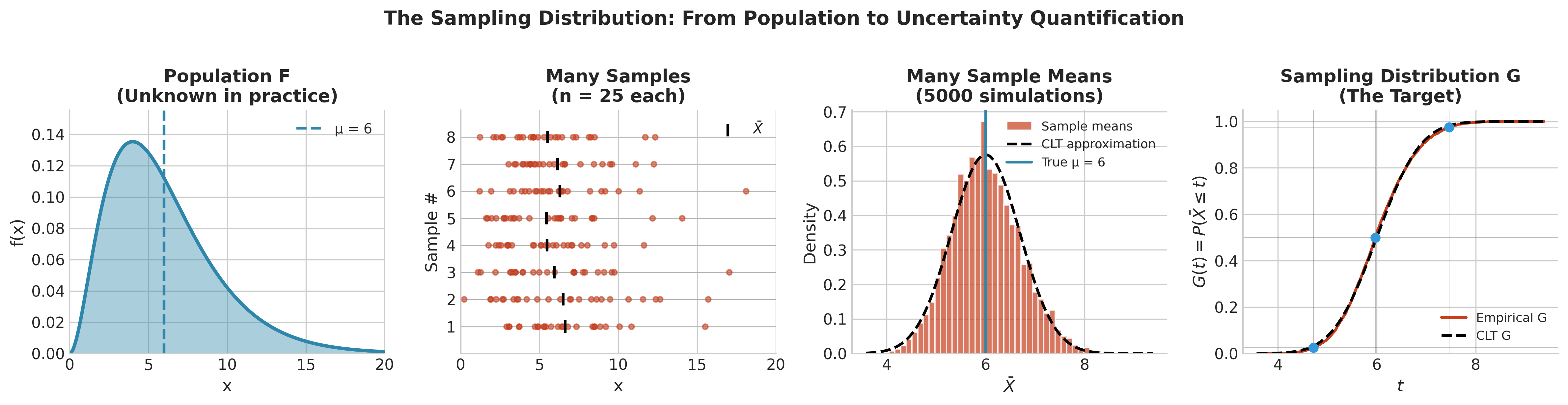
Conceptual diagram showing population F generating many samples, each yielding an estimate, with the collection of estimates forming the sampling distribution G — Fig. 123 **Figure 4.1.1**: The Sampling Distribution Concept. The unknown population \(F\) generates infinitely many possible samples of size \(n\). Each sample yields an estimate \(\hat{\theta}\). The distribution of these estimates across all possible samples is the sampling distribution \(G\). In practice, we observe only one sample and must estimate \(G\) from it.

Everything Flows from G: A Formal Development

Every aspect of uncertainty quantification is a functional of the sampling distribution \(G\). This section develops these connections rigorously, showing that \(G\) is indeed the fundamental target.

Bias

Bias measures systematic error—the tendency of \(\hat{\theta}\) to overestimate or underestimate \(\theta\) on average across repeated samples.

Definition: Bias

The bias of an estimator \(\hat{\theta}\) for parameter \(\theta\) is:

(136)\[\text{Bias}_F(\hat{\theta}) = \mathbb{E}_F[\hat{\theta}] - \theta = \int_{-\infty}^{\infty} t \, dG(t) - \theta\]

An estimator is unbiased if \(\text{Bias}_F(\hat{\theta}) = 0\) for all \(F\) in the model.

The expectation \(\mathbb{E}_F[\hat{\theta}]\) is the mean of the sampling distribution \(G\). If \(G\) has density \(g\), then:

\[\mathbb{E}_F[\hat{\theta}] = \int_{-\infty}^{\infty} t \, g(t) \, dt\]

Bias tells us whether our estimator is “aimed correctly.” An unbiased estimator hits the true parameter on average, though any individual estimate may be above or below \(\theta\).

Variance and Standard Error

Variance quantifies the spread of \(\hat{\theta}\) around its mean across repeated samples—how much \(\hat{\theta}\) fluctuates from sample to sample.

Definition: Variance and Standard Error

The variance of \(\hat{\theta}\) is:

(137)\[\text{Var}_F(\hat{\theta}) = \mathbb{E}_F\left[(\hat{\theta} - \mathbb{E}_F[\hat{\theta}])^2\right] = \int_{-\infty}^{\infty} (t - \mathbb{E}_F[\hat{\theta}])^2 \, dG(t)\]

The standard error is \(\text{SE}(\hat{\theta}) = \sqrt{\text{Var}_F(\hat{\theta})}\).

Standard error is the standard deviation of the sampling distribution. It measures the typical magnitude of deviation of \(\hat{\theta}\) from its expected value.

Mean Squared Error

Mean squared error (MSE) combines bias and variance into a single measure of overall estimator quality.

Definition: Mean Squared Error

The mean squared error of \(\hat{\theta}\) for estimating \(\theta\) is:

(138)\[\text{MSE}_F(\hat{\theta}) = \mathbb{E}_F\left[(\hat{\theta} - \theta)^2\right]\]

Theorem: Bias-Variance Decomposition

(139)\[\text{MSE}_F(\hat{\theta}) = \text{Bias}_F(\hat{\theta})^2 + \text{Var}_F(\hat{\theta})\]

Proof: Let \(\mu = \mathbb{E}_F[\hat{\theta}]\) and \(b = \mu - \theta\) (the bias). Then:

\[\begin{split}\text{MSE} &= \mathbb{E}_F[(\hat{\theta} - \theta)^2] \\ &= \mathbb{E}_F[(\hat{\theta} - \mu + \mu - \theta)^2] \\ &= \mathbb{E}_F[(\hat{\theta} - \mu)^2] + 2(\mu - \theta)\mathbb{E}_F[\hat{\theta} - \mu] + (\mu - \theta)^2 \\ &= \text{Var}_F(\hat{\theta}) + 0 + b^2 \\ &= \text{Var}_F(\hat{\theta}) + \text{Bias}_F(\hat{\theta})^2\end{split}\]

where we used \(\mathbb{E}_F[\hat{\theta} - \mu] = 0\). ∎

This decomposition reveals a fundamental tradeoff:

Low bias, high variance: The estimator is centered correctly but imprecise
High bias, low variance: The estimator is precise but systematically wrong
Optimal: Balance bias and variance to minimize MSE

Confidence Intervals

A confidence interval is a random interval \([L, U]\) constructed from the data such that:

(140)\[P_F\{L \leq \theta \leq U\} \geq 1 - \alpha\]

The probability here is over the sampling distribution. Different samples yield different intervals \([L, U]\)—some contain \(\theta\), some do not. The coverage probability is the proportion of intervals that contain \(\theta\) across all possible samples.

Key Insight: CI Coverage is About G

The coverage probability \(P_F\{L \leq \theta \leq U\}\) is computed with respect to the sampling distribution of \((L, U)\). Since \(L = L(X_1, \ldots, X_n)\) and \(U = U(X_1, \ldots, X_n)\) are functions of the data, they have a joint sampling distribution. The coverage probability is a functional of this distribution.

To construct valid confidence intervals, we need to know or approximate the sampling distribution of our pivotal quantity.

Hypothesis Test p-values

A p-value is the probability, under the null hypothesis, of observing a test statistic as extreme as or more extreme than what was observed:

(141)\[p = P_{F_0}\{T(X_1, \ldots, X_n) \geq T_{\text{obs}}\}\]

where \(F_0\) is the null distribution and \(T_{\text{obs}}\) is the observed test statistic.

This probability is computed with respect to the sampling distribution of \(T\) under \(F_0\). To compute p-values, we need to know \(G_{F_0}\).

The Sampling Distribution in Closed Form: Rare but Illuminating

In a few special cases, we can derive the sampling distribution \(G\) exactly. These cases are illuminating because they show what we’re trying to approximate in general.

Case 1: Sample Mean from Normal Population

Suppose \(X_1, \ldots, X_n \stackrel{\text{iid}}{\sim} N(\mu, \sigma^2)\) and \(\hat{\theta} = \bar{X} = \frac{1}{n}\sum_{i=1}^n X_i\).

Theorem: Exact Sampling Distribution of Sample Mean

If \(X_i \stackrel{\text{iid}}{\sim} N(\mu, \sigma^2)\), then:

(142)\[\bar{X} \sim N\left(\mu, \frac{\sigma^2}{n}\right)\]

Proof: Since \(\bar{X} = \frac{1}{n}\sum_{i=1}^n X_i\) is a linear combination of independent normals, it is normal. Its mean is:

\[\mathbb{E}[\bar{X}] = \frac{1}{n}\sum_{i=1}^n \mathbb{E}[X_i] = \frac{1}{n} \cdot n\mu = \mu\]

Its variance is:

\[\text{Var}(\bar{X}) = \frac{1}{n^2}\sum_{i=1}^n \text{Var}(X_i) = \frac{1}{n^2} \cdot n\sigma^2 = \frac{\sigma^2}{n}\]

∎

This is one of the rare cases where we know \(G\) exactly. From this, everything follows immediately:

Bias: \(\mathbb{E}[\bar{X}] - \mu = 0\) (unbiased)
Standard error: \(\text{SE}(\bar{X}) = \sigma/\sqrt{n}\)
95% CI (if \(\sigma\) known): \(\bar{X} \pm 1.96 \sigma/\sqrt{n}\)
95% CI (if \(\sigma\) unknown): \(\bar{X} \pm t_{n-1, 0.975} \cdot s/\sqrt{n}\) where \(s\) is the sample standard deviation

Case 2: Sample Variance from Normal Population

For \(S^2 = \frac{1}{n-1}\sum_{i=1}^n (X_i - \bar{X})^2\):

Theorem: Distribution of Sample Variance

If \(X_i \stackrel{\text{iid}}{\sim} N(\mu, \sigma^2)\), then:

(143)\[\frac{(n-1)S^2}{\sigma^2} \sim \chi^2_{n-1}\]

and \(S^2\) is independent of \(\bar{X}\).

This result, combined with the distribution of \(\bar{X}\), gives us the t-distribution:

\[\frac{\bar{X} - \mu}{S/\sqrt{n}} \sim t_{n-1}\]

Why These Results Are Exceptional

These closed-form results are exceptional, not typical. They rely on:

Specific distributional assumptions (normality)
Specific statistics (means, variances, linear combinations)
Mathematical properties (closure of normals under linear combinations, Cochran’s theorem for independence)

For most statistics and most populations, no closed-form sampling distribution exists.

Example 💡 Exact Inference When G Is Known

Given: \(X_1, \ldots, X_{16} \stackrel{\text{iid}}{\sim} N(100, 225)\) (IQ scores with \(\mu = 100\), \(\sigma = 15\)).

Find: The sampling distribution of \(\bar{X}\) and a 95% confidence interval for \(\mu\).

Solution:

Since \(\bar{X} \sim N(\mu, \sigma^2/n) = N(100, 225/16) = N(100, 14.0625)\):

Standard error: \(\text{SE} = 15/\sqrt{16} = 3.75\)
95% CI (σ known): \(100 \pm 1.96 \times 3.75 = [92.65, 107.35]\)

Python verification:

import numpy as np
from scipy import stats

# Parameters
mu, sigma, n = 100, 15, 16
se_exact = sigma / np.sqrt(n)

# Exact sampling distribution
sampling_dist = stats.norm(loc=mu, scale=se_exact)

# Confidence interval quantiles
ci_lower = sampling_dist.ppf(0.025)  # 2.5th percentile
ci_upper = sampling_dist.ppf(0.975)  # 97.5th percentile

print(f"Sampling distribution: N({mu}, {se_exact**2:.4f})")
print(f"Standard Error: {se_exact:.4f}")
print(f"95% CI: [{ci_lower:.2f}, {ci_upper:.2f}]")

# Verify by simulation
rng = np.random.default_rng(42)
n_sim = 100000
sample_means = np.array([rng.normal(mu, sigma, n).mean() for _ in range(n_sim)])

print(f"\nSimulation verification ({n_sim:,} samples):")
print(f"Mean of X̄: {sample_means.mean():.2f} (theory: {mu})")
print(f"SD of X̄: {sample_means.std():.4f} (theory: {se_exact:.4f})")

Sampling distribution: N(100, 14.0625)
Standard Error: 3.7500
95% CI: [92.65, 107.35]

Simulation verification (100,000 samples):
Mean of X̄: 100.01 (theory: 100)
SD of X̄: 3.7502 (theory: 3.7500)

This is the ideal scenario: the sampling distribution is known exactly, and all uncertainty quantification follows directly from probability theory.

Historical Development: The Quest for Sampling Distributions

The search for sampling distributions has shaped the history of statistics. Understanding this development illuminates why resampling methods represent such a profound conceptual advance.

The Classical Era: Exact Distributions (1900–1930)

The early 20th century saw remarkable mathematical achievements in deriving exact sampling distributions for specific statistics under specific distributional assumptions.

Pearson’s Chi-Square (1900)

Karl Pearson derived the chi-square distribution for goodness-of-fit testing:

\[\chi^2 = \sum_{i=1}^k \frac{(O_i - E_i)^2}{E_i} \xrightarrow{d} \chi^2_{k-1}\]

under the null hypothesis, where \(O_i\) are observed counts and \(E_i\) are expected counts.

Student’s t-Distribution (1908)

William Sealy Gosset, publishing under the pseudonym “Student,” derived the exact distribution of:

(144)\[T = \frac{\bar{X} - \mu}{S/\sqrt{n}} \sim t_{n-1}\]

when \(X_i \sim N(\mu, \sigma^2)\). This was a breakthrough because it freed the confidence interval from requiring known \(\sigma\). The derivation relied heavily on the normal assumption and the independence of \(\bar{X}\) and \(S^2\) (Cochran’s theorem).

Fisher’s F-Distribution (1920s)

Ronald Fisher derived the distribution of the ratio of independent chi-square variables:

\[F = \frac{\chi^2_m / m}{\chi^2_n / n} \sim F_{m,n}\]

This enabled analysis of variance (ANOVA) and the testing of variance ratios—again, under normality.

The Limitation of Exact Methods

These exact results required:

Specific distributional assumptions (usually normality)
Specific statistics (means, variances, linear combinations)
Mathematical tractability (closure properties, independence results)

For a sample median, a correlation coefficient, or a ratio of means, no closed-form sampling distribution was available. The “distribution-free” methods that emerged (rank tests, etc.) addressed some cases but were limited in scope.

The Asymptotic Era: Central Limit Theorem (1930–1970)

The Central Limit Theorem liberated statistical inference from strict distributional assumptions, at least for large samples. This represented a fundamental shift from exact to approximate inference.

The Classical CLT

Theorem: Central Limit Theorem

Let \(X_1, X_2, \ldots, X_n\) be iid with \(\mathbb{E}[X_i] = \mu\) and \(\text{Var}(X_i) = \sigma^2 < \infty\). Then:

(145)\[\frac{\sqrt{n}(\bar{X} - \mu)}{\sigma} \xrightarrow{d} N(0, 1) \quad \text{as } n \to \infty\]

or equivalently:

\[\sqrt{n}(\bar{X} - \mu) \xrightarrow{d} N(0, \sigma^2)\]

This result holds regardless of the shape of \(F\), provided \(F\) has finite variance. The sampling distribution of \(\bar{X}\) is approximately normal for large \(n\), no matter how non-normal the population.

The Delta Method

For smooth functions \(g\), the CLT extends via Taylor expansion:

Theorem: Delta Method

If \(\sqrt{n}(\hat{\theta} - \theta) \xrightarrow{d} N(0, \sigma^2)\) and \(g\) is continuously differentiable at \(\theta\) with \(g'(\theta) \neq 0\), then:

(146)\[\sqrt{n}(g(\hat{\theta}) - g(\theta)) \xrightarrow{d} N(0, [g'(\theta)]^2 \sigma^2)\]

Proof sketch: By Taylor expansion around \(\theta\):

\[g(\hat{\theta}) - g(\theta) \approx g'(\theta)(\hat{\theta} - \theta)\]

Multiplying by \(\sqrt{n}\) and applying Slutsky’s theorem gives the result. ∎

This enabled approximate inference for transformed quantities: log means, square roots, ratios (via multivariate delta method).

Asymptotic Theory for MLEs

Maximum likelihood estimators have elegant asymptotic properties:

Theorem: Asymptotic Normality of MLE

Under regularity conditions (see Section 3.2):

(147)\[\sqrt{n}(\hat{\theta}_{\text{MLE}} - \theta_0) \xrightarrow{d} N(0, I_1(\theta_0)^{-1})\]

where \(I_1(\theta)\) is the Fisher information per observation.

This provides a universal recipe for inference: compute the MLE, estimate Fisher information, and use the normal approximation.

The Limitation of Asymptotic Methods

Asymptotic results describe behavior as \(n \to \infty\), but we always have finite \(n\). Critical questions include:

How large must \(n\) be? There is no universal answer. The required \(n\) depends on: - The population distribution \(F\) (skewness, kurtosis, tail behavior) - The statistic \(T\) (smooth vs. non-smooth) - The target of inference (center vs. tails of \(G\))
What about non-smooth statistics? The median, quantiles, and other non-smooth statistics have slower convergence or require different asymptotic theory.
What about boundary parameters? When \(\theta\) is near the boundary of the parameter space, standard asymptotic theory fails.

The Computational Era: Resampling (1979–present)

Bradley Efron’s 1979 paper “Bootstrap Methods: Another Look at the Jackknife” inaugurated a new paradigm that fundamentally changed statistical practice.

The Key Insight

Efron’s insight was deceptively simple:

The Bootstrap Idea

If we cannot derive \(G_F\) analytically or trust asymptotic approximations, we can estimate \(G_F\) by Monte Carlo simulation—but using the empirical distribution \(\hat{F}_n\) as a stand-in for the unknown \(F\).

The bootstrap does not derive \(G\); it simulates an approximation to \(G\) by treating \(\hat{F}_n\) as if it were the true population.

Why This Works (Informally)

The empirical distribution \(\hat{F}_n\) converges to \(F\) (Glivenko-Cantelli theorem)
For “nice” functionals \(T\), if \(\hat{F}_n \approx F\), then \(G_{\hat{F}_n} \approx G_F\)
We can compute \(G_{\hat{F}_n}\) by Monte Carlo: resample from \(\hat{F}_n\) (i.e., sample with replacement from the data)

The Conceptual Shift

The shift was profound:

Classical question: “What is the exact or asymptotic form of \(G_F\)?”
Bootstrap question: “What would \(G\) look like if \(F = \hat{F}_n\)?”

The second question can be answered by simulation for virtually any statistic, without requiring distributional assumptions or asymptotic theory.

Historical Impact

The bootstrap arrived at the right moment:

Computational power was becoming widely available (1970s–1980s)
Statisticians recognized the limitations of asymptotic methods
Applied problems increasingly involved complex statistics

Today, bootstrap methods are standard tools in virtually every area of applied statistics.

Three Routes to the Sampling Distribution

We now systematically compare the three canonical approaches to approximating the sampling distribution \(G\). Each has distinct mathematical foundations, computational requirements, and domains of applicability.

Route 1: Analytic/Asymptotic Derivation

Mathematical Foundation

The analytic approach uses probability theory—exact distributional results, the Central Limit Theorem, delta method, and likelihood theory—to derive \(G\) or its large-sample approximation.

Exact Results (when available):

Normal population, sample mean: \(\bar{X} \sim N(\mu, \sigma^2/n)\)
Normal population, sample variance: \((n-1)S^2/\sigma^2 \sim \chi^2_{n-1}\)
Two normals, variance ratio: \(F = S_1^2/S_2^2 \sim F_{n_1-1, n_2-1}\) (under equal variance null)

Asymptotic Results (for large \(n\)):

Sample mean (any \(F\) with finite variance): \(\sqrt{n}(\bar{X} - \mu) \xrightarrow{d} N(0, \sigma^2)\)
MLE (under regularity): \(\sqrt{n}(\hat{\theta} - \theta_0) \xrightarrow{d} N(0, I_1(\theta_0)^{-1})\)
Sample correlation: \(\sqrt{n}(\hat{\rho} - \rho) \xrightarrow{d} N(0, (1-\rho^2)^2)\) for bivariate normal

Practical Implementation

For the sample mean:

\[\hat{\theta} = \bar{X}, \quad \widehat{\text{SE}} = \frac{s}{\sqrt{n}}, \quad \text{CI: } \bar{X} \pm t_{n-1, 1-\alpha/2} \cdot \frac{s}{\sqrt{n}}\]

For MLE \(\hat{\theta}\):

\[\widehat{\text{SE}} = \sqrt{[\hat{I}(\hat{\theta})]^{-1}}, \quad \text{CI: } \hat{\theta} \pm z_{1-\alpha/2} \cdot \widehat{\text{SE}}\]

where \(\hat{I}(\hat{\theta})\) is the observed or expected Fisher information.

Strengths

Computational efficiency: Closed-form formulas are instantaneous
No Monte Carlo variability: Results are deterministic given the data
Theoretical optimality: Under correct assumptions, often achieves optimal efficiency
Deep insight: Formulas reveal how SE depends on \(n\), \(\sigma\), design, etc.

Weaknesses

Requires strong assumptions that may not hold in practice
Limited to specific statistics: Works for smooth functions of moments, not for medians, quantiles, etc.
Asymptotic approximations may be poor for finite \(n\), especially with skewed or heavy-tailed data
Fails near boundaries: Standard theory breaks down when \(\theta\) is near the boundary of the parameter space

Table 37 Statistics with Tractable Analytic/Asymptotic Sampling Distributions
Statistic	Sampling Distribution	Conditions
Sample mean \(\bar{X}\)	\(N(\mu, \sigma^2/n)\) exactly or asymptotically	Normal \(F\) (exact) or finite variance (asymptotic)
Sample variance \(S^2\)	\(\frac{\sigma^2}{n-1} \chi^2_{n-1}\)	Normal \(F\) (exact only)
Sample proportion \(\hat{p}\)	\(N(p, p(1-p)/n)\) asymptotically	\(np\) and \(n(1-p)\) large
MLE \(\hat{\theta}\)	\(N(\theta_0, I_n(\theta_0)^{-1})\) asymptotically	Regularity conditions, large \(n\)
OLS coefficient \(\hat{\beta}\)	\(N(\beta, \sigma^2(\mathbf{X}'\mathbf{X})^{-1})\) exactly	Normal errors, fixed \(\mathbf{X}\)
Pearson correlation \(\hat{\rho}\)	\(N(\rho, (1-\rho^2)^2/n)\) asymptotically	Bivariate normal, large \(n\)

Route 2: Parametric Monte Carlo (Parametric Bootstrap)

Mathematical Foundation

Assume the population belongs to a parametric family: \(F \in \{F_\eta : \eta \in \mathcal{H}\}\). Estimate the parameter \(\hat{\eta}\) from data, then simulate many datasets from \(F_{\hat{\eta}}\), computing the statistic for each.

The Algorithm

Algorithm: Parametric Bootstrap

Input: Data x = (x_1, ..., x_n), parametric family {F_eta}, statistic T, replications B
Output: Monte Carlo approximation to G

1. Fit model: eta_hat = estimate from x (e.g., MLE)
2. For b = 1, 2, ..., B:
   a. Generate x*^(b) = (x_1*^(b), ..., x_n*^(b)) from F_{eta_hat}
   b. Compute theta_hat*^(b) = T(x*^(b))
3. Return {theta_hat*_1, ..., theta_hat*_B} as Monte Carlo sample from G_{F_{eta_hat}}

Use the bootstrap distribution for:
- Standard error: SE_boot = sd{theta_hat*_1, ..., theta_hat*_B}
- Bias estimate: bias_boot = mean{theta_hat*} - theta_hat
- Confidence intervals: various methods

Mathematical Justification

The parametric bootstrap approximates:

\[G_F(t) = P_F\{T(X_1, \ldots, X_n) \leq t\} \approx G_{F_{\hat{\eta}}}(t) = P_{F_{\hat{\eta}}}\{T(X_1^*, \ldots, X_n^*) \leq t\}\]

If the parametric model is correct (i.e., \(F = F_{\eta_0}\) for some \(\eta_0\)) and \(\hat{\eta}\) is consistent, then \(G_{F_{\hat{\eta}}}\) converges to \(G_F\).

Strengths

Applicable to complex statistics: Works for any \(T\) that can be computed
Can generate values outside observed data range: Important for tail inference
Efficient when model is correct: Uses parametric structure for precision
Flexible: Can incorporate complex model features (random effects, dependencies)

Weaknesses

Requires specifying a parametric model: Need to choose \(F_\eta\)
Sensitive to model misspecification: If \(F \notin \{F_\eta\}\), results may be biased
Two sources of error: Model error and Monte Carlo error
More computationally intensive than analytic methods

Example: Parametric Bootstrap for Exponential Rate

import numpy as np
from scipy import stats

def parametric_bootstrap_exponential(x, B=10000, seed=42):
    """
    Parametric bootstrap for exponential rate parameter.

    Parameters
    ----------
    x : array
        Observed data (assumed exponential)
    B : int
        Number of bootstrap replicates
    seed : int
        Random seed

    Returns
    -------
    dict with rate_hat, se_boot, ci_percentile, boot_dist
    """
    rng = np.random.default_rng(seed)
    n = len(x)

    # MLE for exponential rate
    rate_hat = 1 / x.mean()

    # Parametric bootstrap: sample from Exp(rate_hat)
    rate_boot = np.empty(B)
    for b in range(B):
        x_star = rng.exponential(scale=1/rate_hat, size=n)
        rate_boot[b] = 1 / x_star.mean()

    se_boot = rate_boot.std(ddof=1)
    ci_percentile = np.percentile(rate_boot, [2.5, 97.5])

    return {
        'rate_hat': rate_hat,
        'se_boot': se_boot,
        'ci_percentile': ci_percentile,
        'boot_dist': rate_boot
    }

# Example usage
rng = np.random.default_rng(42)
true_rate = 0.5
n = 30
x = rng.exponential(scale=1/true_rate, size=n)

result = parametric_bootstrap_exponential(x, B=10000)
print(f"True rate: {true_rate}")
print(f"MLE: {result['rate_hat']:.4f}")
print(f"Bootstrap SE: {result['se_boot']:.4f}")
print(f"95% CI: [{result['ci_percentile'][0]:.4f}, {result['ci_percentile'][1]:.4f}]")

Route 3: Nonparametric Bootstrap

Mathematical Foundation

Replace the unknown \(F\) with the empirical distribution \(\hat{F}_n\), which places mass \(1/n\) at each observed data point:

(148)\[\hat{F}_n(x) = \frac{1}{n} \sum_{i=1}^n \mathbf{1}\{X_i \leq x\}\]

Simulate datasets by resampling with replacement from \(\{X_1, \ldots, X_n\}\).

The Algorithm

Algorithm: Nonparametric Bootstrap

Input: Data x = (x_1, ..., x_n), statistic T, replications B
Output: Bootstrap distribution {theta_hat*_1, ..., theta_hat*_B}

1. Compute point estimate: theta_hat = T(x)
2. For b = 1, 2, ..., B:
   a. Generate x*^(b) by sampling n values from {x_1, ..., x_n} with replacement
   b. Compute theta_hat*^(b) = T(x*^(b))
3. Return {theta_hat*_1, ..., theta_hat*_B}

Mathematical Justification

The nonparametric bootstrap approximates:

(149)\[G_F(t) = P_F\{T(X_1, \ldots, X_n) \leq t\} \approx G_{\hat{F}_n}(t) = P_{\hat{F}_n}\{T(X_1^*, \ldots, X_n^*) \leq t\}\]

The justification rests on:

Consistency of \(\hat{F}_n\): By Glivenko-Cantelli, \(\|\hat{F}_n - F\|_\infty \to 0\) almost surely
Continuity of the functional: For “smooth” functionals, \(G_{\hat{F}_n} \to G_F\) when \(\hat{F}_n \to F\)

We develop this rigorously in Section 4.2.

Strengths

No parametric model required: Completely nonparametric
Automatic adaptation: Captures skewness, heavy tails, heterogeneity in the data
Universal applicability: Works for essentially any statistic \(T\)
Captures finite-sample behavior: Reflects actual data characteristics, not asymptotic idealizations
Easy to implement: Requires only the ability to compute \(T\)

Weaknesses

Cannot generate values outside the observed data range: Bootstrap samples are limited to observed values
May fail for extreme-value statistics: Max, min, high quantiles have non-regular behavior
Requires modification for dependent or designed data: Standard bootstrap assumes iid
Computationally intensive: Requires \(B\) evaluations of \(T\)

Implementation

import numpy as np
from typing import Callable, Dict

def bootstrap_distribution(
    x: np.ndarray,
    statistic: Callable[[np.ndarray], float],
    B: int = 10000,
    seed: int = None
) -> np.ndarray:
    """
    Generate the bootstrap distribution of a statistic.

    Parameters
    ----------
    x : np.ndarray
        Original data sample of shape (n,) or (n, p)
    statistic : callable
        Function that computes the statistic from a sample.
        Should accept an array and return a scalar.
    B : int
        Number of bootstrap replicates (default 10000)
    seed : int, optional
        Random seed for reproducibility

    Returns
    -------
    np.ndarray
        Bootstrap replicates of shape (B,)

    Examples
    --------
    >>> rng = np.random.default_rng(42)
    >>> x = rng.normal(0, 1, 50)
    >>> boot_means = bootstrap_distribution(x, np.mean, B=5000, seed=42)
    >>> print(f"Bootstrap SE: {boot_means.std(ddof=1):.4f}")
    """
    rng = np.random.default_rng(seed)
    n = len(x)

    theta_boot = np.empty(B)
    for b in range(B):
        # Resample with replacement
        indices = rng.choice(n, size=n, replace=True)
        x_star = x[indices]
        theta_boot[b] = statistic(x_star)

    return theta_boot


def bootstrap_inference(
    x: np.ndarray,
    statistic: Callable[[np.ndarray], float],
    B: int = 10000,
    alpha: float = 0.05,
    seed: int = None
) -> Dict:
    """
    Complete bootstrap inference for a statistic.

    Parameters
    ----------
    x : np.ndarray
        Original data
    statistic : callable
        Statistic function
    B : int
        Number of bootstrap replicates
    alpha : float
        Significance level for confidence interval
    seed : int
        Random seed

    Returns
    -------
    dict with keys:
        'theta_hat': point estimate
        'se_boot': bootstrap standard error
        'bias_boot': bootstrap bias estimate
        'ci_percentile': percentile confidence interval
        'ci_basic': basic (pivotal) confidence interval
        'boot_dist': bootstrap distribution
    """
    theta_hat = statistic(x)
    boot_dist = bootstrap_distribution(x, statistic, B, seed)

    se_boot = boot_dist.std(ddof=1)
    bias_boot = boot_dist.mean() - theta_hat

    # Percentile interval
    ci_percentile = np.percentile(boot_dist, [100*alpha/2, 100*(1-alpha/2)])

    # Basic (pivotal) interval
    q_lower = np.percentile(boot_dist, 100*alpha/2)
    q_upper = np.percentile(boot_dist, 100*(1-alpha/2))
    ci_basic = (2*theta_hat - q_upper, 2*theta_hat - q_lower)

    return {
        'theta_hat': theta_hat,
        'se_boot': se_boot,
        'bias_boot': bias_boot,
        'ci_percentile': ci_percentile,
        'ci_basic': ci_basic,
        'boot_dist': boot_dist
    }

Formal Comparison of the Three Routes

Table 38 Comprehensive Comparison of Approaches to the Sampling Distribution
Aspect	Analytic/Asymptotic	Parametric Monte Carlo	Nonparametric Bootstrap
Population assumption	Known form or CLT applies	\(F \in \{F_\eta\}\) (parametric family)	None (uses \(\hat{F}_n\))
What is approximated	\(G_F\) exactly or asymptotically	\(G_{F_{\hat{\eta}}}\) via simulation	\(G_{\hat{F}_n}\) via resampling
Key assumption	Distributional form or regularity	Parametric model is correct	\(\hat{F}_n \approx F\) (large \(n\))
Tail behavior	Theory-driven (extrapolates)	Model-driven (extrapolates)	Data-limited (no extrapolation)
Smooth statistics	Often works well	Works well if model fits	Works well
Non-smooth statistics	Often fails or complex	Works if model fits	Usually works
Small \(n\)	Asymptotics unreliable	Depends on model adequacy	May be unstable
Computational cost	\(O(1)\) (formula)	\(O(B \cdot C(n))\) where \(C(n)\) = cost of \(T\)	\(O(B \cdot C(n))\)
MC variability	None	Yes (reducible by increasing \(B\))	Yes (reducible by increasing \(B\))

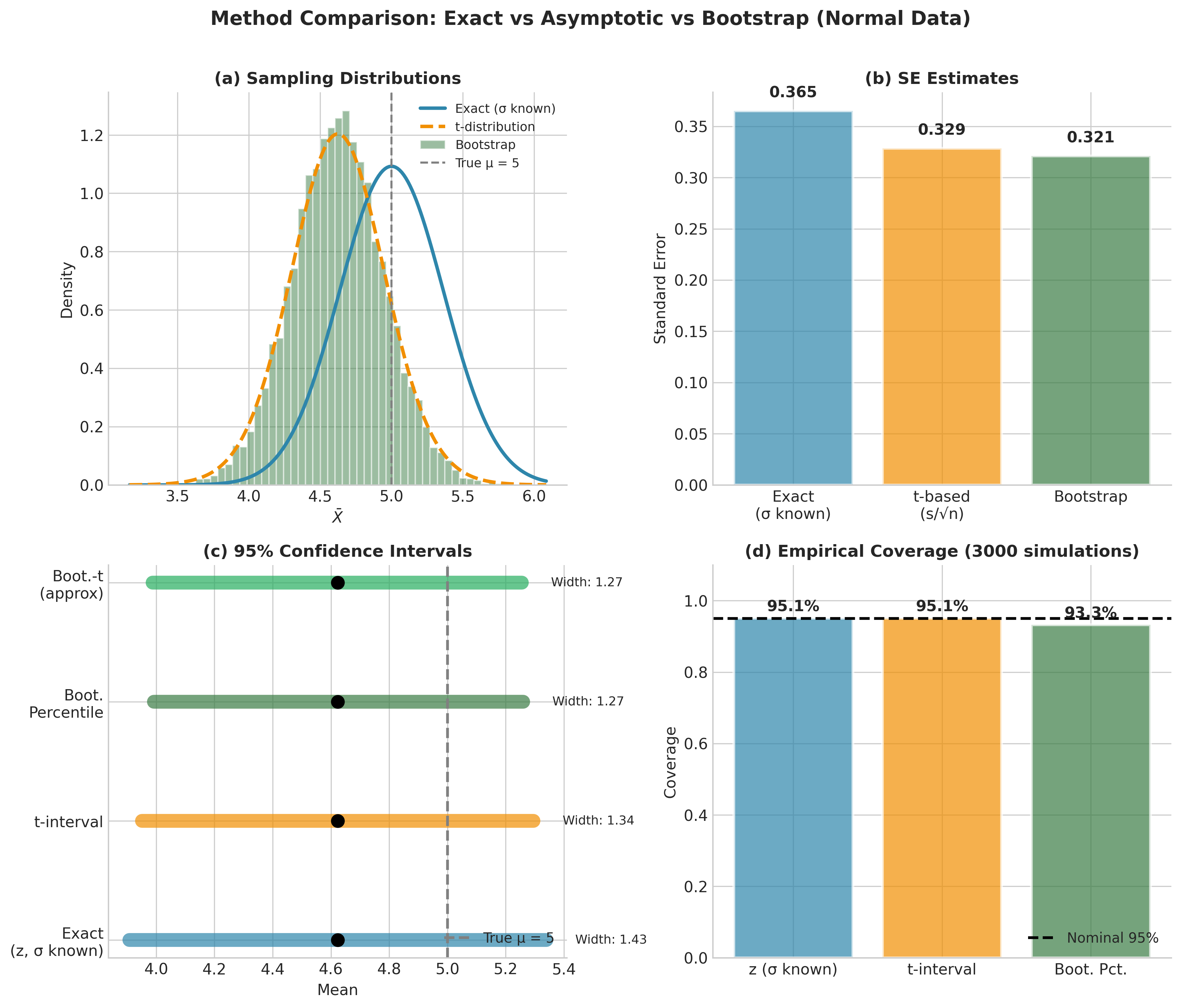
Side-by-side comparison of analytic, parametric bootstrap, and nonparametric bootstrap confidence intervals for different scenarios — Fig. 124 **Figure 4.1.9**: Method Comparison Across Scenarios. Each panel shows 95% confidence intervals from three methods for a different inference problem. Panel A: Sample mean from normal data—all methods agree. Panel B: Sample median from skewed data—bootstrap intervals are appropriately asymmetric while analytic intervals are symmetric. Panel C: Ratio of means—bootstrap captures the right-skewed distribution that the delta method misses. The bootstrap adapts automatically to the structure of each problem.

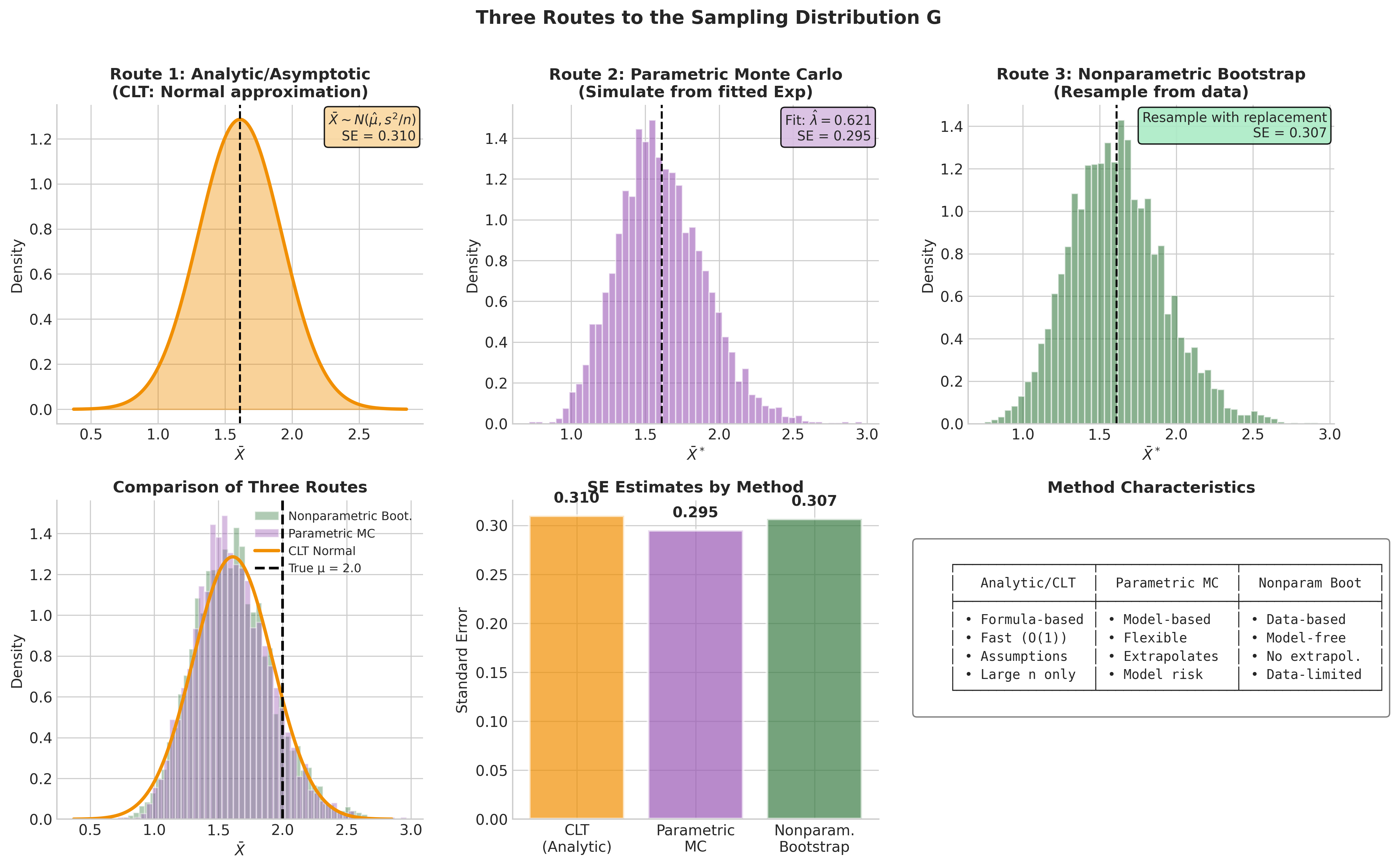
Flowchart showing three routes from population F to sampling distribution G — Fig. 125 **Figure 4.1.2**: Three Routes to the Sampling Distribution. The analytic route derives \(G\) using probability theory—fast but assumption-heavy. Parametric Monte Carlo simulates from a fitted model—flexible but model-dependent. The bootstrap simulates from the empirical distribution—model-free but data-limited.

When Asymptotics Fail: Motivating the Bootstrap

The bootstrap becomes essential when analytic and asymptotic methods fail or are unreliable. This section examines specific scenarios where classical methods break down, providing mathematical analysis and empirical demonstrations.

Scenario 1: Non-Smooth Statistics

Consider estimating the population median \(m = F^{-1}(0.5)\) using the sample median \(\hat{m}\).

The Asymptotic Theory

The sample median has asymptotic distribution:

Theorem: Asymptotic Distribution of Sample Median

If \(F\) has a density \(f\) that is positive and continuous at \(m = F^{-1}(0.5)\), then:

(150)\[\sqrt{n}(\hat{m} - m) \xrightarrow{d} N\left(0, \frac{1}{4[f(m)]^2}\right)\]

The asymptotic standard error is:

\[\text{SE}_{\text{asymp}}(\hat{m}) = \frac{1}{2f(m)\sqrt{n}}\]

The Problem

This formula requires knowing \(f(m)\)—the density evaluated at the median—which is unknown and difficult to estimate reliably:

Density estimation is hard: Requires choosing a bandwidth, is sensitive to outliers, and has slow convergence rates
Evaluation at \(m\) is even harder: We must estimate \(f\) at a specific point (the median), compounding estimation error
The formula is sensitive: Small errors in \(\hat{f}(m)\) lead to large errors in \(\widehat{\text{SE}}\) because \(f(m)\) appears in the denominator

Bootstrap Solution

The bootstrap sidesteps density estimation entirely:

Resample with replacement from the data
Compute the sample median for each resample
Use the empirical standard deviation of bootstrap medians as the SE estimate

No density estimation required!

Example 💡 Median Inference: Asymptotic vs. Bootstrap

Setup: \(n = 50\) observations from a lognormal distribution (right-skewed).

import numpy as np
from scipy import stats
from scipy.stats import gaussian_kde

rng = np.random.default_rng(42)

# True population parameters
mu_log, sigma_log = 1.5, 0.8
true_median = np.exp(mu_log)  # Median of lognormal = exp(mu)
true_density_at_median = stats.lognorm.pdf(true_median, s=sigma_log,
                                            scale=np.exp(mu_log))
n = 50

# Generate sample
x = rng.lognormal(mu_log, sigma_log, n)
median_hat = np.median(x)

print("="*60)
print("MEDIAN INFERENCE: ASYMPTOTIC VS BOOTSTRAP")
print("="*60)
print(f"\nTrue median: {true_median:.3f}")
print(f"Sample median: {median_hat:.3f}")
print(f"True f(m): {true_density_at_median:.4f}")

# Asymptotic SE: requires density estimation
# Method 1: Kernel density estimation
kde = gaussian_kde(x)
f_hat_kde = kde(median_hat)[0]
se_asymp_kde = 1 / (2 * f_hat_kde * np.sqrt(n))

# Method 2: Using true density (oracle - not available in practice)
se_asymp_oracle = 1 / (2 * true_density_at_median * np.sqrt(n))

print(f"\nAsymptotic SE (KDE): {se_asymp_kde:.4f}")
print(f"Asymptotic SE (oracle): {se_asymp_oracle:.4f}")

# Bootstrap SE
B = 10000
median_boot = np.array([np.median(rng.choice(x, size=n, replace=True))
                         for _ in range(B)])
se_boot = median_boot.std(ddof=1)

print(f"Bootstrap SE: {se_boot:.4f}")

# Confidence intervals
z_crit = stats.norm.ppf(0.975)
ci_asymp = (median_hat - z_crit*se_asymp_kde, median_hat + z_crit*se_asymp_kde)
ci_boot = np.percentile(median_boot, [2.5, 97.5])

print(f"\n95% CI (asymptotic): [{ci_asymp[0]:.3f}, {ci_asymp[1]:.3f}]")
print(f"95% CI (bootstrap):  [{ci_boot[0]:.3f}, {ci_boot[1]:.3f}]")

# Check if bootstrap captures skewness
boot_skewness = stats.skew(median_boot)
print(f"\nBootstrap distribution skewness: {boot_skewness:.3f}")
print("(Positive skew reflects the right-skewed population)")

============================================================
MEDIAN INFERENCE: ASYMPTOTIC VS BOOTSTRAP
============================================================

True median: 4.482
Sample median: 4.668
True f(m): 0.1265

Asymptotic SE (KDE): 0.6177
Asymptotic SE (oracle): 0.5597
Bootstrap SE: 0.6834

95% CI (asymptotic): [3.457, 5.878]
95% CI (bootstrap):  [3.551, 6.276]

Bootstrap distribution skewness: 0.634
(Positive skew reflects the right-skewed population)

Key observations:

The KDE-based SE differs from the oracle SE by about 10%—density estimation introduces substantial uncertainty
The bootstrap SE is slightly larger, reflecting additional uncertainty the asymptotic formula misses
The bootstrap distribution is right-skewed (skewness = 0.63), capturing the population’s skewness that the symmetric normal CI ignores

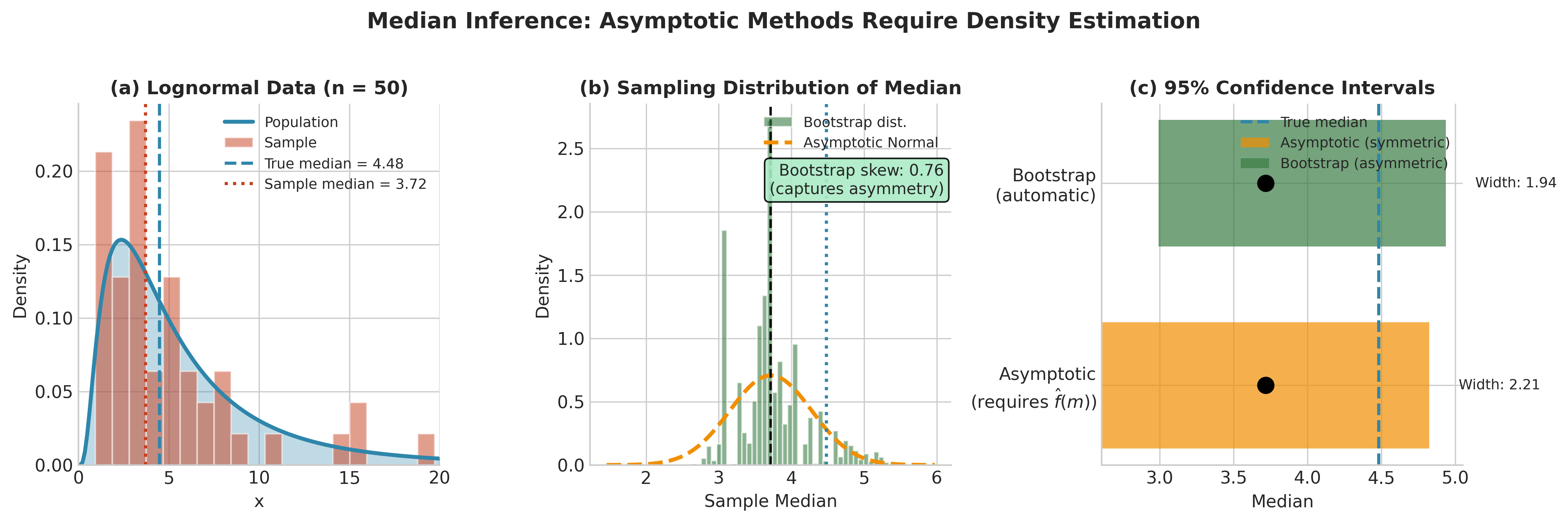
Comparison of asymptotic and bootstrap inference for the sample median, showing bootstrap distribution with skewness versus symmetric normal approximation — Fig. 126 **Figure 4.1.3**: Median Inference—Asymptotic vs. Bootstrap. Left: The bootstrap distribution of the sample median captures the right-skewness inherited from the lognormal population. Right: The asymptotic normal approximation (red curve) assumes symmetry. The bootstrap percentile interval (shaded) is appropriately asymmetric, while the asymptotic interval (dashed lines) is symmetric around the estimate.

Scenario 2: Ratios of Random Variables

Consider estimating the ratio of two population means: \(\theta = \mu_X / \mu_Y\).

The Delta Method Approach

For independent samples, the delta method gives:

\[\hat{\theta} = \frac{\bar{X}}{\bar{Y}}, \quad \text{Var}(\hat{\theta}) \approx \hat{\theta}^2 \left(\frac{\sigma_X^2}{n_X \mu_X^2} + \frac{\sigma_Y^2}{n_Y \mu_Y^2}\right)\]

For paired data \((X_i, Y_i)\):

(151)\[\text{Var}(\hat{\theta}) \approx \frac{1}{n\mu_Y^2}\left(\sigma_X^2 + \theta^2\sigma_Y^2 - 2\theta\sigma_{XY}\right)\]

The Problems

Denominator variability: When \(\bar{Y}\) is variable (small \(n_Y\), large \(\sigma_Y\)), \(\hat{\theta}\) can be very unstable
Near-zero denominators: If \(\bar{Y} \approx 0\) in some samples, the ratio explodes
Non-normality: The ratio of normals is not normal (it follows a Cauchy-like distribution when means are near zero)
Skewness: Even when well-behaved, ratios are typically right-skewed; symmetric CIs are inappropriate

Bootstrap Solution

Resample paired observations \((X_i, Y_i)\), compute \(\bar{X}^*/\bar{Y}^*\) for each resample, and use the bootstrap distribution directly. This automatically captures:

The joint variability of numerator and denominator
The skewness of the ratio distribution
The instability when \(\bar{Y}\) is near zero

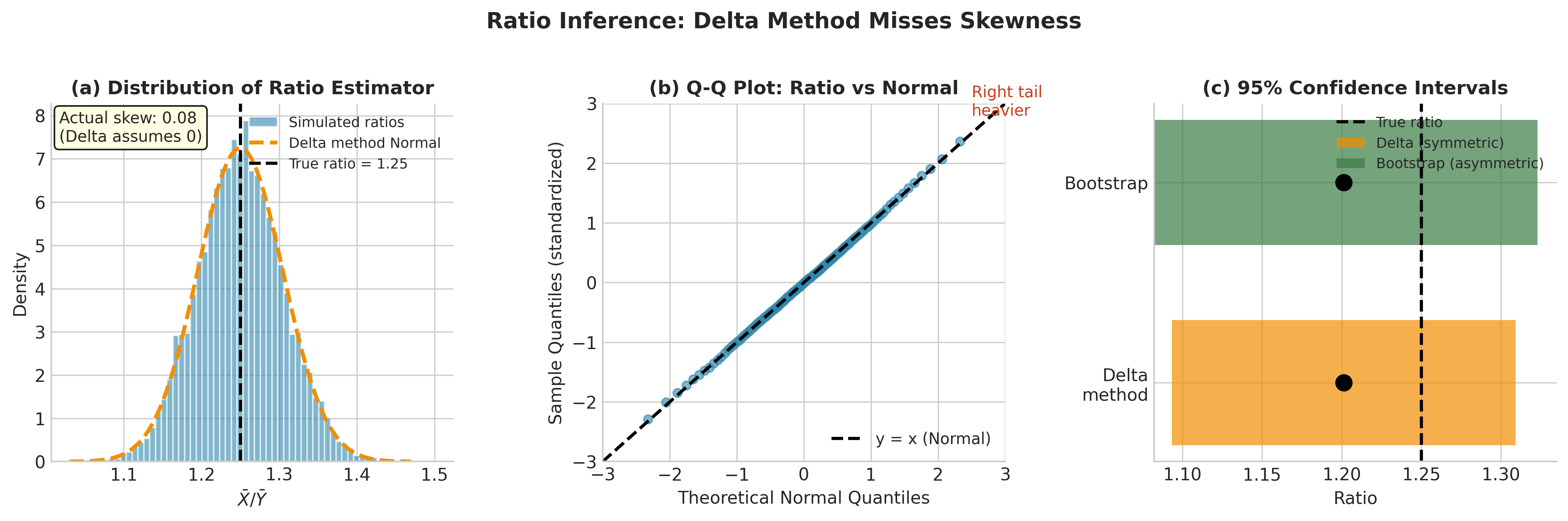
Bootstrap distribution of ratio estimator showing right-skewed distribution compared to symmetric delta method approximation — Fig. 127 **Figure 4.1.4**: Ratio Inference—Delta Method vs. Bootstrap. The bootstrap distribution (histogram) reveals the inherent right-skewness of the ratio \(\bar{X}/\bar{Y}\). The delta method normal approximation (red curve) incorrectly assumes symmetry. When denominator variability is substantial, the delta method can severely underestimate the probability of extreme values.

Scenario 3: Small Samples from Non-Normal Populations

Asymptotic theory describes behavior as \(n \to \infty\). For small \(n\), the CLT approximation may be poor, especially for:

Skewed populations: The symmetric normal approximation is inappropriate
Heavy-tailed populations: The sample mean has higher variance than the CLT suggests
Discrete populations: The approximation can be noticeably discrete for small \(n\)

Theoretical Background: Berry-Esseen Bound

The Berry-Esseen theorem quantifies the rate of convergence in the CLT:

Theorem: Berry-Esseen Bound

If \(X_1, \ldots, X_n\) are iid with \(\mathbb{E}[X] = \mu\), \(\text{Var}(X) = \sigma^2\), and \(\mathbb{E}[|X - \mu|^3] = \rho < \infty\), then:

(152)\[\sup_t \left| P\left\{\frac{\sqrt{n}(\bar{X} - \mu)}{\sigma} \leq t\right\} - \Phi(t) \right| \leq \frac{C \cdot \rho}{\sigma^3 \sqrt{n}}\]

where \(C < 0.4748\) (Shevtsova, 2011) and \(\Phi\) is the standard normal CDF.

The bound shows that convergence is \(O(1/\sqrt{n})\) and is slower when the population has high skewness (large \(\rho/\sigma^3\)).

Simulation Study: Coverage of t-Intervals

import numpy as np
from scipy import stats

def coverage_study(distribution, params, n_values, n_sim=10000, alpha=0.05):
    """
    Study coverage of t-intervals for various sample sizes.
    """
    rng = np.random.default_rng(42)
    results = {}

    for n in n_values:
        covers = 0
        true_mean = distribution.mean(**params)

        for _ in range(n_sim):
            sample = distribution.rvs(size=n, random_state=rng, **params)
            xbar = sample.mean()
            se = sample.std(ddof=1) / np.sqrt(n)
            t_crit = stats.t.ppf(1 - alpha/2, df=n-1)

            ci_lower = xbar - t_crit * se
            ci_upper = xbar + t_crit * se

            if ci_lower <= true_mean <= ci_upper:
                covers += 1

        results[n] = covers / n_sim

    return results

# Test on exponential (skewed) and t_3 (heavy-tailed)
n_values = [10, 20, 30, 50, 100, 200]

print("="*60)
print("T-INTERVAL COVERAGE BY SAMPLE SIZE")
print("="*60)
print(f"\nNominal coverage: 95%")

# Exponential(1): skewness = 2
exp_coverage = coverage_study(stats.expon, {'scale': 1}, n_values)
print(f"\nExponential(1) [skewness = 2]:")
for n, cov in exp_coverage.items():
    flag = " ⚠" if cov < 0.93 else ""
    print(f"  n = {n:3d}: {cov:.3f}{flag}")

Interpretation: For skewed (exponential) and heavy-tailed (t_3) populations, t-intervals undercover for small \(n\). Coverage approaches 95% only for \(n \geq 50-100\). Normal data achieves correct coverage even for \(n = 10\).

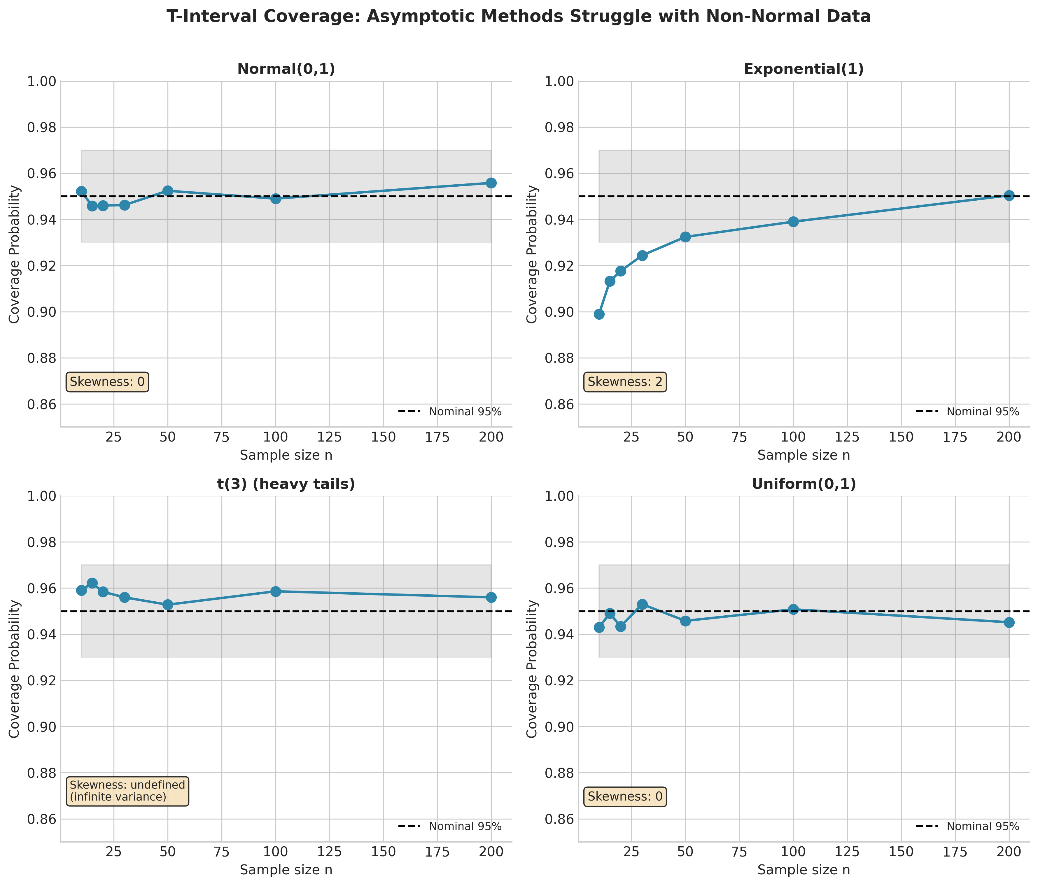
Coverage probability of t-intervals across sample sizes for normal, exponential, and t(3) distributions showing undercoverage for non-normal populations at small n — Fig. 128 **Figure 4.1.5**: T-Interval Coverage Depends on Population Shape. Coverage probability (y-axis) versus sample size (x-axis) for three populations. The horizontal line marks nominal 95% coverage. Normal populations achieve correct coverage even at \(n = 10\). Exponential (skewed) and \(t_3\) (heavy-tailed) populations show substantial undercoverage for \(n < 50\), with coverage gradually improving toward the nominal level as \(n\) increases.

Scenario 4: Boundary and Extreme-Value Statistics

When parameters lie on or near the boundary of the parameter space, or when the statistic involves extreme values, standard asymptotic theory fails.

Example: Sample Maximum

For \(\hat{\theta} = X_{(n)} = \max(X_1, \ldots, X_n)\):

The Maximum Is Non-Regular

The sample maximum has a non-standard asymptotic distribution. Under appropriate conditions:

\[a_n(X_{(n)} - b_n) \xrightarrow{d} G\]

where \(G\) is a generalized extreme value (GEV) distribution—not normal! The normalizing constants \(a_n, b_n\) depend on the tail behavior of \(F\).

The CLT does not apply to extreme-value statistics.

Bootstrap Considerations for Extremes

The nonparametric bootstrap can also struggle with extreme-value statistics because:

\(\hat{F}_n\) cannot generate values outside the observed range
The bootstrap maximum \(X_{(n)}^*\) has a point mass at \(X_{(n)}\) (probability that the largest observation is resampled at least once)

For extreme-value inference, specialized methods (parametric bootstrap with GEV family, subsampling, or m-out-of-n bootstrap) may be needed.

A Decision Framework

Given the analysis above, when should each approach be used?

START: Need SE or CI for theta_hat = T(X_1,...,X_n)

|
+--> Is T a smooth function of sample moments?
|   |
|   +--> YES: Is n large AND population well-behaved?
|   |   |
|   |   +--> YES: Use ANALYTIC methods (CLT, delta method)
|   |   |
|   |   +--> NO (small n, heavy tails): Use BOOTSTRAP
|   |
|   +--> NO: T is non-smooth (median, quantile, etc.)
|       |
|       +--> Use BOOTSTRAP
|
+--> Is there a credible parametric model?
|   |
|   +--> YES: Use PARAMETRIC BOOTSTRAP (good for tails)
|   |
|   +--> NO: Use NONPARAMETRIC BOOTSTRAP
|
+--> Are observations dependent?
|   |
|   +--> Clustered: CLUSTER BOOTSTRAP
|   +--> Time series: BLOCK BOOTSTRAP
|   +--> Stratified: STRATIFIED BOOTSTRAP
|
+--> Is theta_hat an extreme-value statistic?
    |
    +--> Standard bootstrap may fail: Consider specialized methods

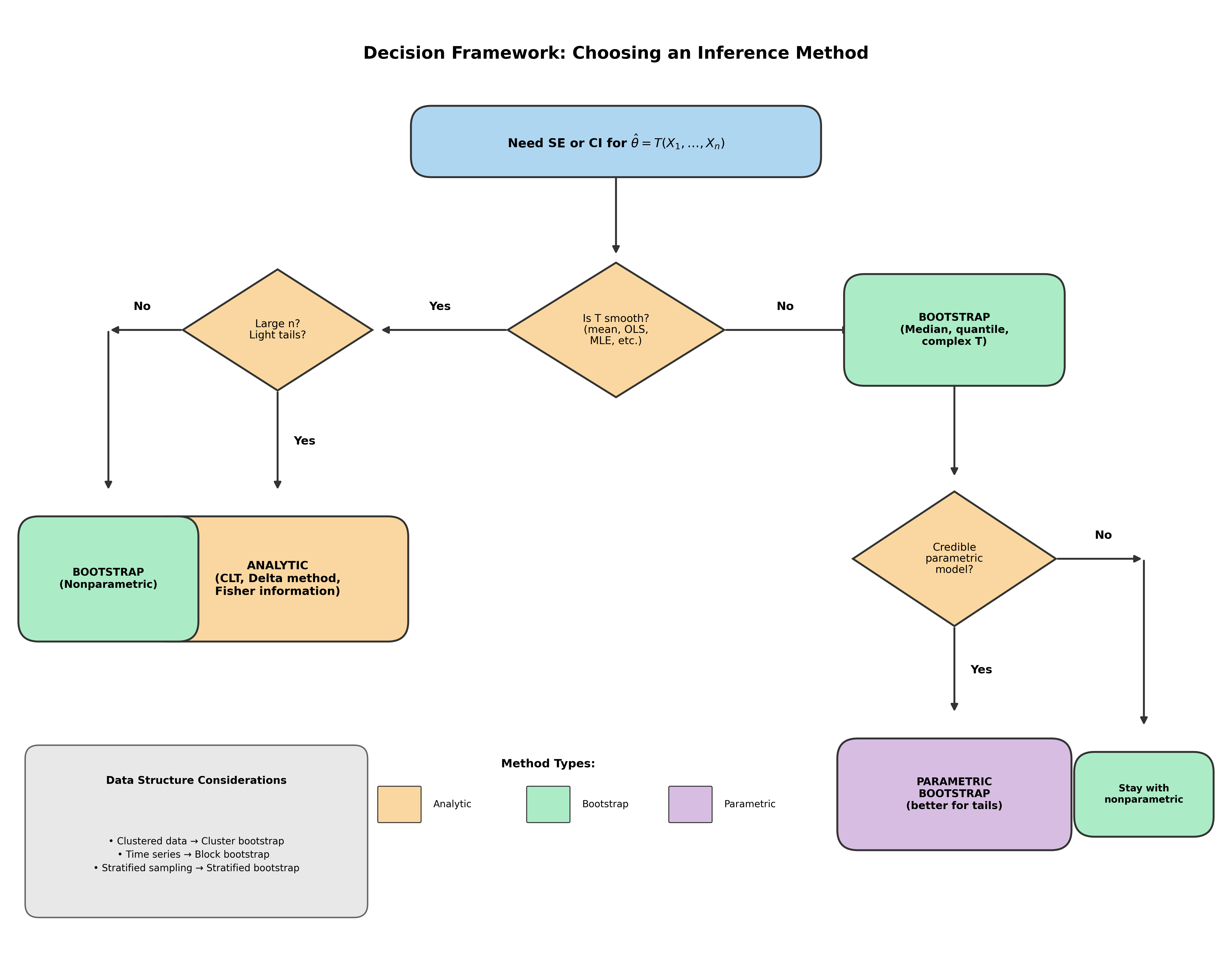
Decision flowchart for choosing between analytic, parametric bootstrap, and nonparametric bootstrap methods based on statistic type, sample size, and data structure — Fig. 129 **Figure 4.1.10**: Decision Framework for Choosing an Inference Method. This flowchart guides practitioners through key questions: Is the statistic smooth? Is \(n\) large? Is there a credible parametric model? Are observations independent? The answers determine whether analytic methods suffice or whether bootstrap (parametric or nonparametric) is needed, and which bootstrap variant is appropriate.

The Plug-In Principle: Theoretical Foundation

The bootstrap is not a black box or ad-hoc method—it rests on a principled idea called the plug-in principle. Understanding this principle clarifies why the bootstrap works and when it might fail.

Statistical Functionals

Most population quantities of interest can be expressed as functionals—functions that take a probability distribution as input and return a number.

Definition: Statistical Functional

A statistical functional is a map \(T: \mathcal{F} \to \mathbb{R}\) that assigns a real number to each distribution in some class \(\mathcal{F}\).

The parameter \(\theta\) is then \(\theta = T(F)\).

Examples of Statistical Functionals:

Table 39 Common Parameters as Functionals
Parameter	Functional Notation	Definition
Mean	\(T(F) = \int x \, dF(x)\)	\(\mathbb{E}_F[X]\)
Variance	\(T(F) = \int (x - \mu_F)^2 \, dF(x)\)	\(\text{Var}_F(X)\)
Median	\(T(F) = F^{-1}(0.5)\)	\(\inf\{x : F(x) \geq 0.5\}\)
Correlation	\(T(F) = \frac{\text{Cov}_F(X,Y)}{\text{SD}_F(X) \cdot \text{SD}_F(Y)}\)	\(\text{Corr}_F(X, Y)\)

The Plug-In Estimator

The plug-in principle provides a general recipe for estimation:

The Plug-In Principle (Parameter Level)

To estimate a functional \(\theta = T(F)\), substitute the empirical distribution \(\hat{F}_n\) for \(F\):

(153)\[\hat{\theta} = T(\hat{F}_n)\]

The empirical distribution function is:

(154)\[\hat{F}_n(x) = \frac{1}{n} \sum_{i=1}^n \mathbf{1}\{X_i \leq x\}\]

This is the CDF of a discrete distribution placing mass \(1/n\) on each observed data point.

Verifying Plug-In for Common Statistics:

Sample mean as plug-in estimator of population mean:

\[T(F) = \int x \, dF(x) \quad \Rightarrow \quad T(\hat{F}_n) = \int x \, d\hat{F}_n(x) = \frac{1}{n}\sum_{i=1}^n x_i = \bar{x}\]

Sample variance as plug-in estimator (with divisor \(n\)):

\[T(F) = \int (x - \mu_F)^2 \, dF(x) \quad \Rightarrow \quad T(\hat{F}_n) = \frac{1}{n}\sum_{i=1}^n (x_i - \bar{x})^2\]

Extending to Uncertainty Quantification

The key insight of the bootstrap is to extend the plug-in principle from parameters to sampling distributions:

The Plug-In Principle (Distribution Level)

Parameter plug-in: The parameter \(\theta = T(F)\) is estimated by \(\hat{\theta} = T(\hat{F}_n)\).

Uncertainty plug-in: The sampling distribution \(G_F\) of \(\hat{\theta}\) is estimated by \(G_{\hat{F}_n}\).

Since we cannot draw new samples from the unknown \(F\), we draw samples from \(\hat{F}_n\)—which means sampling with replacement from the observed data.

The relationship is:

\[\underbrace{G_{\hat{F}_n}}_{\text{bootstrap distribution}} \text{ approximates } \underbrace{G_F}_{\text{true sampling distribution}}\]

just as

\[\underbrace{\hat{F}_n}_{\text{empirical distribution}} \text{ approximates } \underbrace{F}_{\text{true population}}\]

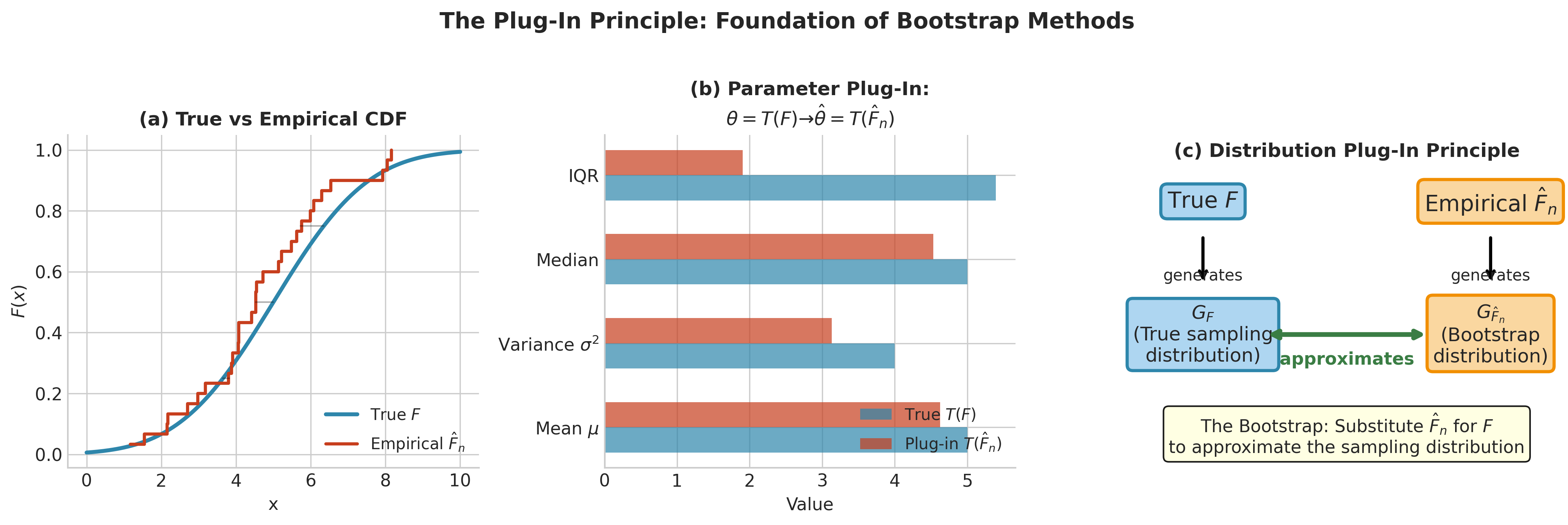
Diagram illustrating the plug-in principle at both parameter and distribution levels, showing F to theta and F_hat to theta_hat parallels — Fig. 130 **Figure 4.1.6**: The Plug-In Principle at Two Levels. Top row: Parameter estimation—the unknown \(F\) yields parameter \(\theta = T(F)\), which we estimate by \(\hat{\theta} = T(\hat{F}_n)\) using the empirical distribution. Bottom row: Uncertainty estimation—the unknown sampling distribution \(G_F\) is approximated by \(G_{\hat{F}_n}\), obtained by resampling from \(\hat{F}_n\). Both levels rest on the same principle: substitute \(\hat{F}_n\) for \(F\).

Why This Should Work (Informal Argument)

\(\hat{F}_n \to F\) as \(n \to \infty\) (Glivenko-Cantelli theorem)
If \(G\) depends “continuously” on \(F\), then \(G_{\hat{F}_n} \to G_F\)
We can compute \(G_{\hat{F}_n}\) by Monte Carlo (resampling from \(\hat{F}_n\))

The formal development of when this works is the subject of Section 4.2.

Theoretical Justification: Preview

The rigorous justification for the bootstrap involves several deep results from probability theory, which we develop fully in Section 4.2. Here we preview the key ideas.

Glivenko-Cantelli Theorem: The empirical distribution converges uniformly to the true distribution.

Theorem: Glivenko-Cantelli (Preview)

With probability 1:

(155)\[\|\hat{F}_n - F\|_\infty = \sup_x \left| \hat{F}_n(x) - F(x) \right| \xrightarrow{a.s.} 0 \quad \text{as } n \to \infty\]

Bootstrap Consistency: Under regularity conditions, for a broad class of statistics:

\[\sup_t |G_{\hat{F}_n}(t) - G_F(t)| \xrightarrow{P} 0\]

The bootstrap distribution converges to the true sampling distribution in probability.

When the Bootstrap Fails

The bootstrap can fail when:

Sample size too small: \(\hat{F}_n\) is too coarse an approximation to \(F\)
Functional not continuous: Extreme-value statistics, for example
Tail dependence: Bootstrap cannot generate values outside observed range
Dependence structure: Standard bootstrap assumes iid

Computational Perspective: Bootstrap as Monte Carlo

From a computational standpoint, the bootstrap is simply Monte Carlo integration where the target distribution is \(\hat{F}_n\) rather than some theoretical \(F\).

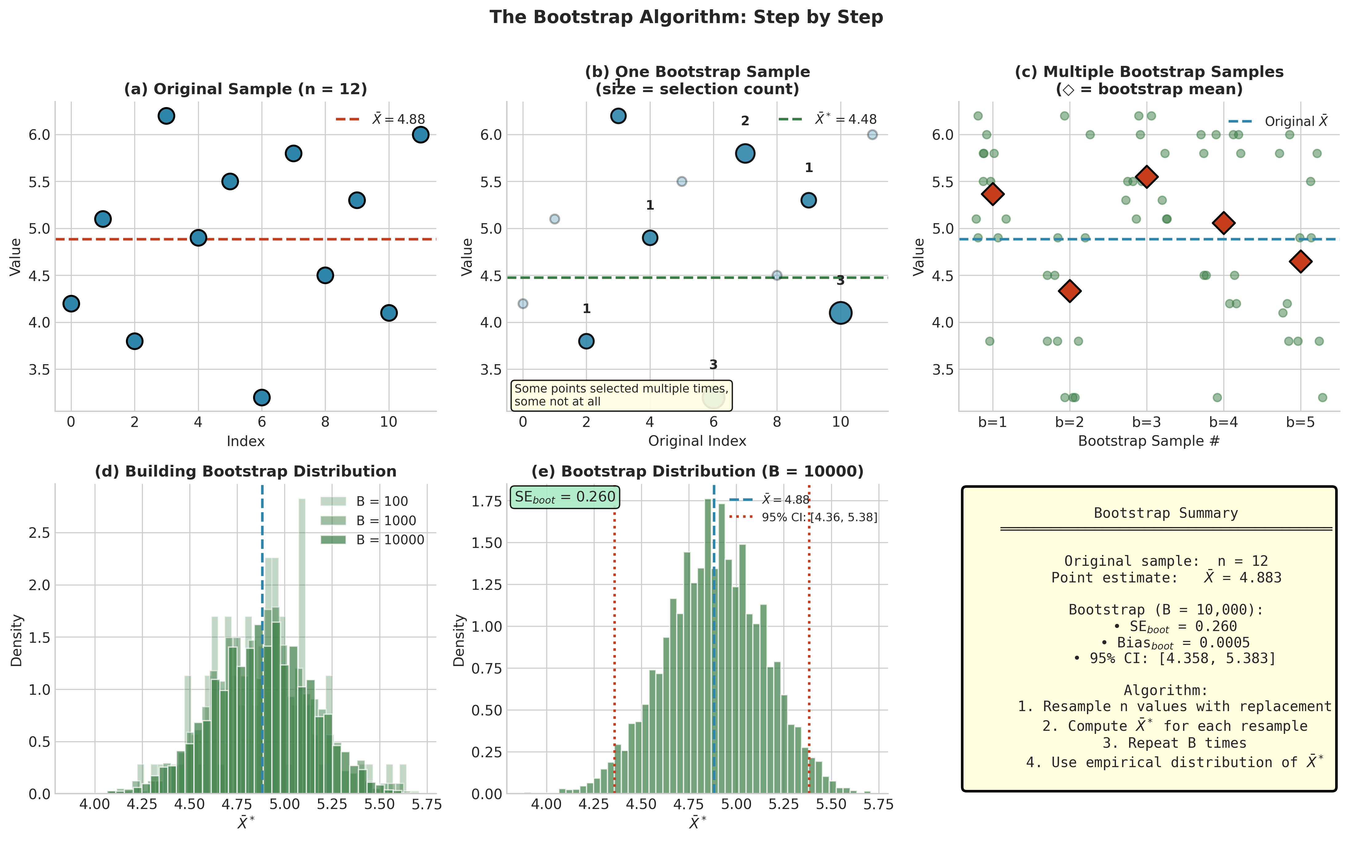
Step-by-step visualization of the bootstrap algorithm showing original sample, resampling with replacement, computing statistics, and building the bootstrap distribution — Fig. 131 **Figure 4.1.7**: The Bootstrap Algorithm Visualized. Starting from the original sample (left), we repeatedly resample with replacement to create bootstrap samples (middle). For each bootstrap sample, we compute the statistic of interest. After \(B\) replications, the collection of bootstrap statistics forms the bootstrap distribution (right), which approximates the true sampling distribution \(G\).

Two Layers of Randomness

A crucial point for understanding and reporting bootstrap results: the bootstrap involves two distinct sources of randomness:

Two Sources of Uncertainty

1. Statistical Uncertainty (what we want to estimate)

Source: Finite sample size \(n\); different samples from \(F\) give different \(\hat{\theta}\)
Quantified by: The true standard error \(\text{SE}(\hat{\theta}) = \sqrt{\text{Var}_F(\hat{\theta})}\)
Controlled by: Collecting more data (larger \(n\))
Magnitude: Typically \(O(1/\sqrt{n})\)

2. Monte Carlo Uncertainty (computational noise)

Source: Finite number of bootstrap replicates \(B\)
Quantified by: The Monte Carlo standard error of \(\widehat{\text{SE}}_{\text{boot}}\)
Controlled by: Increasing \(B\)
Magnitude: Typically \(O(1/\sqrt{B})\)

Monte Carlo Error of the SE Estimate

The bootstrap SE estimate has its own variability:

(156)\[\text{SE}(\widehat{\text{SE}}_{\text{boot}}) \approx \frac{\widehat{\text{SE}}_{\text{boot}}}{\sqrt{2(B-1)}}\]

For \(B = 1000\):

\[\text{Coefficient of Variation} = \frac{1}{\sqrt{2 \times 999}} \approx 2.2\%\]

For \(B = 10000\):

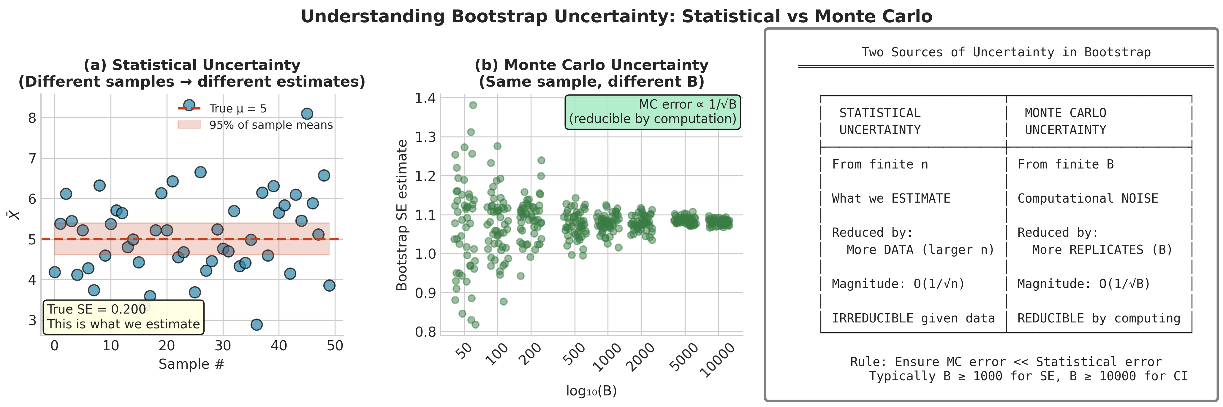
\[\text{Coefficient of Variation} = \frac{1}{\sqrt{2 \times 9999}} \approx 0.7\%\]

Diagram distinguishing statistical uncertainty from finite n versus Monte Carlo uncertainty from finite B, showing how each is controlled — Fig. 132 **Figure 4.1.8**: Two Layers of Randomness in Bootstrap Inference. Statistical uncertainty (left) arises from observing a finite sample \(n\) from the population—this is what we want to estimate. Monte Carlo uncertainty (right) arises from using finite bootstrap replicates \(B\)—this is computational noise we can reduce. Increasing \(B\) reduces Monte Carlo error but cannot reduce statistical uncertainty; only collecting more data (larger \(n\)) addresses statistical uncertainty.

Choosing B

Guidelines based on the target:

Table 40 Guidelines for Choosing B
Target	Recommended B	Rationale
Standard error estimation	200–1,000	SE estimate has low MC variance
Percentile CI (95%)	1,000–2,000	Need accurate 2.5th and 97.5th percentiles
Percentile CI (99%)	5,000–10,000	More extreme percentiles need more samples
BCa intervals	2,000–10,000	Acceleration constant estimation
Publication-quality results	10,000+	Minimize MC variability in reported values

Common Pitfall ⚠️ Confusing the Two Sources of Uncertainty

Misconception: “I ran the bootstrap with \(B = 100,000\) replicates, so my standard error must be very accurate.”

Reality: Large \(B\) reduces Monte Carlo uncertainty but does not reduce statistical uncertainty. If \(n\) is small and \(\hat{F}_n\) is a poor approximation to \(F\), the bootstrap estimate of SE may be biased regardless of \(B\).

Rule of Thumb:

\(B\) controls Monte Carlo precision (computational noise)
\(n\) controls statistical accuracy (how well \(\hat{F}_n \approx F\))
Increasing \(B\) beyond ~10,000 rarely helps; collecting more data (larger \(n\)) does

Practical Considerations

Before implementing bootstrap methods, practitioners should understand several practical issues that affect reliability and interpretation.

Sample Size Requirements

The bootstrap assumes \(\hat{F}_n \approx F\), which requires \(n\) to be large enough that the sample adequately represents the population.

General Guidelines:

Table 41 Minimum Sample Sizes for Bootstrap
Statistic Type	Minimum n	Notes
Smooth (mean, regression)	15–20	Works well for most distributions
Quantiles (median, quartiles)	30–50	More for extreme quantiles
Correlation, covariance	25–30	Need bivariate structure captured
Ratios	30+	Denominator variability matters
Multivariate (p parameters)	5p–10p	Rule of thumb: several times # parameters

When the Bootstrap May Fail

The bootstrap is not universally applicable. Key failure modes include:

1. Extreme-Value Statistics

The sample maximum \(X_{(n)}\) or minimum \(X_{(1)}\) have non-regular behavior. Bootstrap distribution places positive probability mass at the observed extremes.

2. Boundary Parameters

When \(\theta\) is near or at the boundary of parameter space (proportions near 0 or 1, variance near 0, correlation near ±1).

3. Heavy Tails with Infinite Variance

If \(\text{Var}_F(X) = \infty\) (e.g., Cauchy distribution), the bootstrap for \(\bar{X}\) may not converge correctly.

4. Dependent Data

The standard bootstrap assumes iid observations. For time series, clustered data, or spatial data, specialized bootstrap methods are required.

Bringing It All Together

This section has established the conceptual and mathematical foundations for resampling methods. The key developments are:

The Fundamental Target

The sampling distribution \(G(t) = P_F\{\hat{\theta} \leq t\}\) is the fundamental target of uncertainty quantification. Everything we want to know about estimator uncertainty—standard errors, confidence intervals, p-values, bias—is a functional of \(G\).

Three Routes to G

We identified three canonical approaches:

Analytic/Asymptotic: Derive \(G\) using probability theory. Fast and assumption-rich; works well for smooth statistics, large samples, correct model specification.
Parametric Monte Carlo: Simulate from a fitted parametric model \(F_{\hat{\eta}}\). Flexible and can extrapolate into tails. Carries the risk of model misspecification.
Nonparametric Bootstrap: Simulate from the empirical distribution \(\hat{F}_n\). Model-free, automatic, broadly applicable. Cannot extrapolate beyond observed data.

When Classical Methods Fail

We documented scenarios where asymptotics are unreliable: non-smooth statistics, ratios, small samples from non-normal populations, and extreme-value statistics.

The Plug-In Principle

The bootstrap rests on extending plug-in estimation from parameters to distributions:

Parameter level: \(\theta = T(F) \to \hat{\theta} = T(\hat{F}_n)\)
Distribution level: \(G_F \to G_{\hat{F}_n}\)

Looking Ahead

Section 4.2 develops the empirical distribution and plug-in principle rigorously, proving Glivenko-Cantelli and the DKW inequality. Subsequent sections develop confidence interval methods, diagnostics, and specialized variants for regression, dependent data, and hypothesis testing.

Key Takeaways 📝

Core concept: The sampling distribution \(G(t) = P_F\{\hat{\theta} \leq t\}\) is the fundamental target of all uncertainty quantification. Standard errors, confidence intervals, p-values, and bias are all functionals of \(G\).
Three routes: Analytic methods derive \(G\) from theory (fast but assumption-heavy); parametric Monte Carlo simulates from a fitted model (flexible but model-dependent); bootstrap simulates from \(\hat{F}_n\) (model-free but data-limited).
When asymptotics fail: Non-smooth statistics (median), ratios, small samples from non-normal populations, and boundary parameters all cause classical asymptotic methods to perform poorly. The bootstrap provides a robust alternative.
Plug-in principle: The bootstrap extends plug-in estimation from parameters (\(\theta = T(F) \to T(\hat{F}_n)\)) to sampling distributions (\(G_F \to G_{\hat{F}_n}\)). This is justified by the consistency of \(\hat{F}_n\) for \(F\).
Two sources of uncertainty: Statistical uncertainty (from finite \(n\)) is what we want to estimate. Monte Carlo uncertainty (from finite \(B\)) is computational noise we can reduce by increasing \(B\).
Course outcome alignment: This section addresses Learning Outcome 1 (simulation techniques) by framing the bootstrap as Monte Carlo on \(\hat{F}_n\), and Learning Outcome 3 (resampling for variability and CIs) by establishing the conceptual foundation for all resampling inference.

Chapter 4.1 Exercises

These exercises develop your understanding of the sampling distribution problem and the foundations of resampling methods.

Exercise 1: Fundamentals of Sampling Distributions

Explain why the sampling distribution \(G\) is called “the fundamental target of uncertainty quantification.” Identify which aspects of inference derive from \(G\).
Suppose \(X_1, \ldots, X_{25} \stackrel{\text{iid}}{\sim} \text{Exp}(1)\). Let \(\hat{\theta} = \bar{X}\). What are the exact mean and variance of the sampling distribution of \(\hat{\theta}\)?
A colleague claims “the standard error is a property of the sample.” Correct this misconception.
If we observe \(\bar{x} = 1.15\) from our sample of 25, explain what “95% coverage probability” means for a confidence interval.

Exercise 2: Comparing the Three Routes

For each scenario, identify which route to the sampling distribution would be most appropriate:

Estimating the mean of a normal population with \(n = 100\), \(\sigma\) unknown
Estimating the sample median from \(n = 50\) observations from an unknown heavy-tailed distribution
Estimating the ratio \(\mu_X / \mu_Y\) from paired data with \(n = 40\)
Estimating the 99th percentile of a lognormal distribution from \(n = 500\)

Exercise 3: Monte Carlo vs. Statistical Uncertainty

A colleague says “I computed a bootstrap SE with \(B = 50,000\) replicates, so it must be very precise.”

Is this reasoning correct? Explain the distinction between Monte Carlo error and statistical uncertainty.
For \(B = 50,000\), what is the approximate Monte Carlo coefficient of variation of the SE estimate?
If \(n = 20\) and the true SE is 0.5, would increasing \(B\) from 10,000 to 100,000 meaningfully improve inference?

Exercise 4: Plug-In Estimators

Show that the sample mean \(\bar{X}\) is the plug-in estimator of \(\mu = \int x \, dF(x)\).
Show that the plug-in estimator of variance has divisor \(n\), not \(n-1\).
Explain why plug-in estimators are generally biased. Give an example.

Exercise 5: Coverage Simulation

Conduct a simulation comparing t-interval and bootstrap percentile CI coverage for the mean.

Test on: Exponential(1), t(3), and Normal(0,1)
Use sample sizes \(n \in \{10, 25, 50, 100\}\)
For which distributions and sample sizes does the t-interval undercover?

References

Foundational Bootstrap Papers

[Efron1979]

Efron, B. (1979). Bootstrap methods: Another look at the jackknife. The Annals of Statistics, 7(1), 1–26.

[EfronTibshirani1993]

Efron, B., and Tibshirani, R. J. (1993). An Introduction to the Bootstrap. Chapman & Hall/CRC.

Theoretical Foundations

[Hall1992]

Hall, P. (1992). The Bootstrap and Edgeworth Expansion. Springer.

[VanDerVaart1998]

van der Vaart, A. W. (1998). Asymptotic Statistics. Cambridge University Press.

Convergence Results

[Glivenko1933]

Glivenko, V. (1933). Sulla determinazione empirica delle leggi di probabilità. Giornale dell’Istituto Italiano degli Attuari, 4, 92–99.

[Dvoretzky1956]

Dvoretzky, A., Kiefer, J., and Wolfowitz, J. (1956). Asymptotic minimax character of the sample distribution function. The Annals of Mathematical Statistics, 27(3), 642–669.

Modern References

[EfronHastie2016]

Efron, B., and Hastie, T. (2016). Computer Age Statistical Inference. Cambridge University Press.

[Davison1997]

Davison, A. C., and Hinkley, D. V. (1997). Bootstrap Methods and their Application. Cambridge University Press.