Section 4.4: The Parametric Bootstrap

The nonparametric bootstrap of nonparametric-bootstrap treats the empirical distribution \(\hat{F}_n\) as a proxy for the unknown population \(F\). This approach requires minimal assumptions but ignores any structural knowledge about \(F\). When a credible parametric model is available, we can do better: the parametric bootstrap simulates from a fitted parametric distribution \(F_{\hat{\theta}}\), potentially achieving greater efficiency and better finite-sample performance.

This section develops the parametric bootstrap as a natural extension of the plug-in principle, explores its theoretical advantages and failure modes, and provides practical guidance for choosing between parametric and nonparametric approaches.

Road Map 🧭

• Understand: The parametric bootstrap principle and its relationship to the plug-in estimator

• Develop: Algorithms for location-scale families, regression, and GLMs

• Implement: Efficient Python code for parametric bootstrap inference

• Evaluate: Model diagnostics and the efficiency-robustness tradeoff

The Parametric Bootstrap Principle

Conceptual Framework

Recall the bootstrap philosophy: we approximate the sampling distribution \(G_F\) of a statistic \(\hat{\theta} = T(X_{1:n})\) by studying its behavior under a proxy distribution. In the nonparametric bootstrap, this proxy is \(\hat{F}_n\), the empirical distribution placing mass \(1/n\) on each observation.

The parametric bootstrap takes a different approach. Given a parametric family \(\{F_\theta : \theta \in \Theta\}\), we:

1. Fit the model: Estimate \(\hat{\theta}_n\) from the data (typically via MLE).

2. Simulate from the fitted model: Generate \(X_1^*, \ldots, X_n^* \stackrel{iid}{\sim} F_{\hat{\theta}_n}\).

3. Compute bootstrap statistics: Calculate \(\hat{\theta}^*_b = T(X_1^*, \ldots, X_n^*)\).

4. Approximate the sampling distribution: Use \(\{\hat{\theta}^*_1, \ldots, \hat{\theta}^*_B\}\) for inference.

Key Distinction

• Nonparametric bootstrap: Resample from \(\hat{F}_n\) (the data itself)

• Parametric bootstrap: Simulate fresh data from \(F_{\hat{\theta}_n}\) (the fitted model)

The parametric bootstrap generates genuinely new observations—not rearrangements of the original data. Each bootstrap sample is a fresh draw from the estimated population.

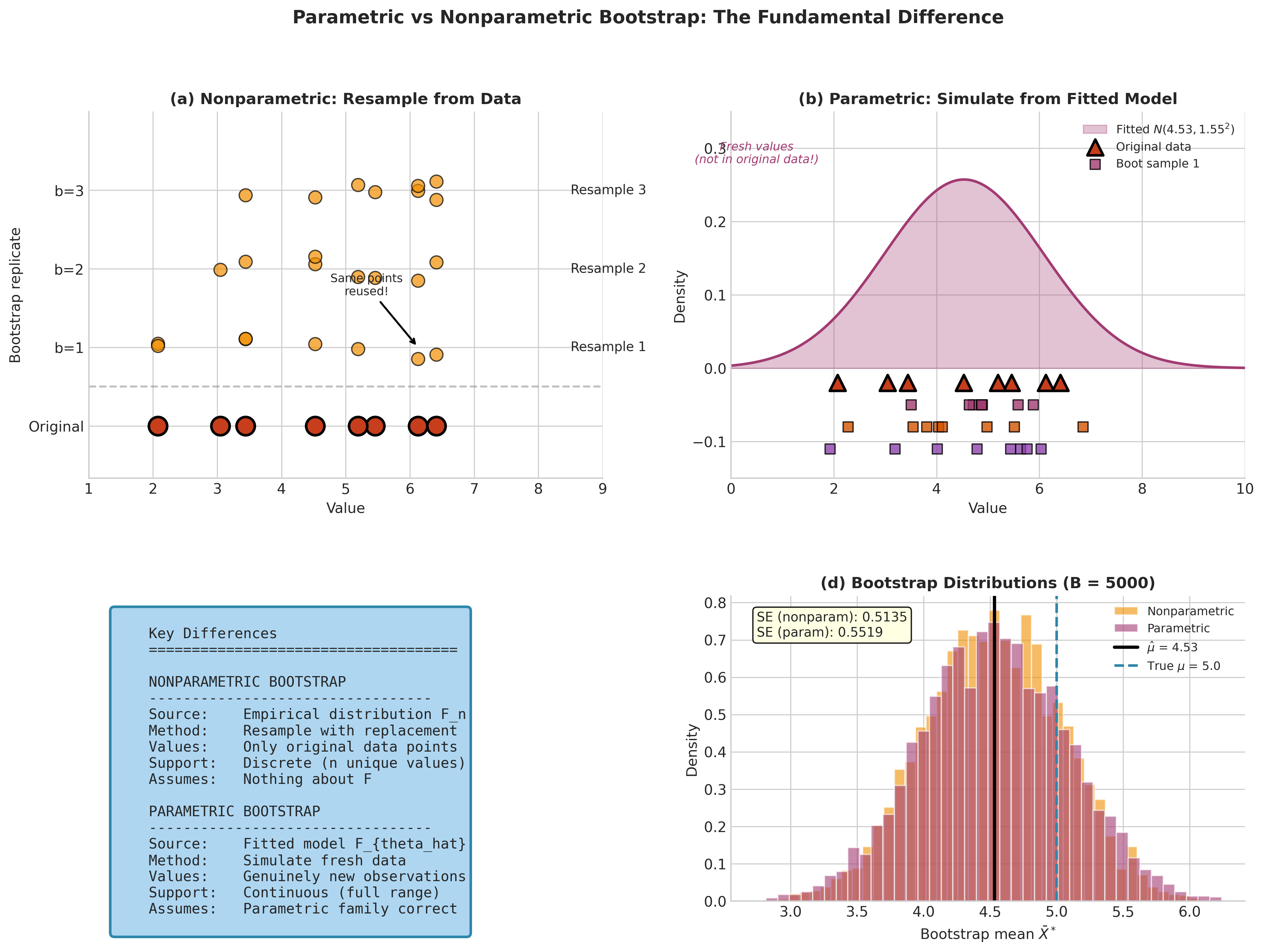
Fig. 151 Figure 4.4.1: The fundamental difference between parametric and nonparametric bootstrap. Panel (a) shows nonparametric bootstrap resampling the same data points with replacement. Panel (b) shows parametric bootstrap generating fresh observations from the fitted distribution. Panel (d) compares the resulting bootstrap distributions.

Mathematical Framework

Let \(X_1, \ldots, X_n \stackrel{iid}{\sim} F_{\theta_0}\) where \(\theta_0 \in \Theta\) is the true parameter. The goal is to approximate the sampling distribution of \(\hat{\theta}_n = T(X_{1:n})\).

The parametric bootstrap distribution is the conditional distribution of \(\hat{\theta}^*_n\) given \(\hat{\theta}_n\):

\[G^*_{\hat{\theta}_n}(t) = P_{\hat{\theta}_n}\left(\hat{\theta}^*_n \leq t \mid \hat{\theta}_n\right)\]

where \(\hat{\theta}^*_n = T(X_1^*, \ldots, X_n^*)\) with \(X_i^* \stackrel{iid}{\sim} F_{\hat{\theta}_n}\).

Consistency: Under regularity conditions (continuous \(F_\theta\), consistent \(\hat{\theta}_n\), smooth \(T\)), the parametric bootstrap is consistent:

\[\sup_t \left| G^*_{\hat{\theta}_n}(t) - G_{\theta_0}(t) \right| \xrightarrow{P} 0\]

where \(G_{\theta_0}\) is the true sampling distribution of \(\hat{\theta}_n\).

Higher-order accuracy: For studentized statistics \(Z^* = \sqrt{n}(\hat{\theta}^* - \hat{\theta}_n)/\hat{\sigma}^*\), studentization combined with bootstrap calibration can achieve second-order accuracy under standard regularity conditions (smooth parametric models, asymptotically pivotal statistics):

\[\sup_t \left| P^*(Z^* \leq t) - P(Z \leq t) \right| = O_P(n^{-1})\]

compared to \(O_P(n^{-1/2})\) for unstudentized percentile methods, which are typically first-order accurate. This improved convergence rate is a major advantage for confidence interval construction, though it requires proper studentization with per-replicate SE estimates.

Why Use Parametric Bootstrap?

Efficiency when the model is correct: If \(F_{\hat{\theta}_n}\) is close to \(F_{\theta_0}\), the parametric bootstrap produces tighter confidence intervals than the nonparametric bootstrap.

Better finite-sample behavior: With small samples (\(n < 50\)), the empirical distribution \(\hat{F}_n\) is a crude approximation to \(F\). A well-chosen parametric model can capture population features (tails, smoothness) that \(\hat{F}_n\) misses.

Natural for model-based inference: When the analysis already assumes a parametric model (regression, GLM, survival analysis), parametric bootstrap maintains consistency between model fitting and uncertainty quantification.

Handles boundary constraints: Parametric models naturally respect parameter constraints (e.g., variances are positive, probabilities are in \([0,1]\)), while nonparametric bootstrap may produce invalid resamples.

Parametric Bootstrap vs. Parametric Monte Carlo

Students sometimes ask: “Is parametric bootstrap just parametric Monte Carlo?” The distinction is subtle but important:

• Parametric Monte Carlo simulates from a known parametric model with \(\theta\) treated as given or hypothesized (e.g., simulating under the null hypothesis).

• Parametric bootstrap simulates from an estimated model \(F_{\hat{\theta}}\), approximating the sampling distribution under the true \(F_{\theta_0}\).

This distinction explains why model misspecification is fatal for parametric bootstrap: we’re using \(\hat{\theta}\) as a proxy for \(\theta_0\), and if the model family is wrong, this proxy breaks down.

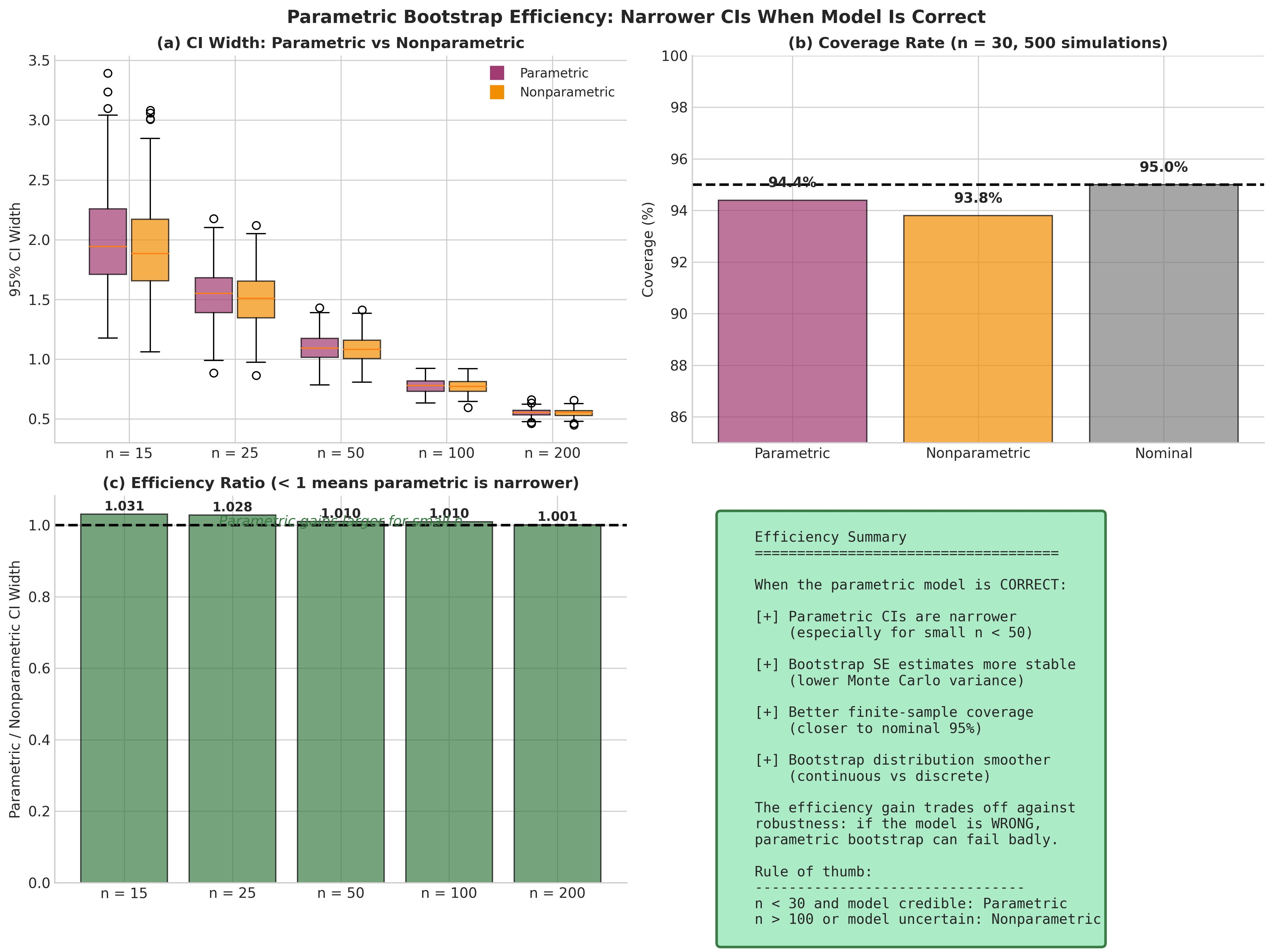
Fig. 152 Figure 4.4.3: Efficiency comparison when the parametric model is correct. (a) CI widths across sample sizes—parametric produces narrower intervals, especially for small n. (b) Coverage rates near nominal 95%. (c) Efficiency ratio shows parametric gains are largest for small samples.

The Algorithm: General Form

Algorithm: Parametric Bootstrap (General)

Input: Data X₁, ..., Xₙ; parametric family {F_θ}; estimator θ̂; statistic T; replicates B
Output: Bootstrap distribution {T*₁, ..., T*_B}

1. Fit model: Compute θ̂ₙ from data (e.g., MLE)
2. For b = 1, ..., B:
   a. Generate X*₁, ..., X*ₙ iid ~ F_{θ̂ₙ}
   b. Compute θ̂*_b from bootstrap sample
   c. Compute T*_b = T(θ̂*_b) or any functional of interest
3. Return {T*₁, ..., T*_B}

Computational complexity: \(O(B \cdot n \cdot c)\) where \(c\) is the cost of computing \(T\). For regression with \(p\) predictors, \(c = O(np^2)\) for OLS.

Python Implementation

import numpy as np
from scipy import stats

def parametric_bootstrap(data, fit_model, generate_data, statistic,
                         B=2000, seed=None):
    """
    General parametric bootstrap.

    Parameters
    ----------
    data : array_like
        Original data.
    fit_model : callable
        Function that takes data and returns fitted parameters.
    generate_data : callable
        Function that takes (params, n, rng) and returns simulated data.
    statistic : callable
        Function that computes the statistic from data.
    B : int
        Number of bootstrap replicates.
    seed : int, optional
        Random seed for reproducibility.

    Returns
    -------
    theta_star : ndarray
        Bootstrap distribution of the statistic.
    theta_hat : float or ndarray
        Original estimate.
    params_hat : tuple
        Fitted model parameters.
    """
    rng = np.random.default_rng(seed)
    data = np.asarray(data)
    n = len(data)

    # Step 1: Fit model to original data
    params_hat = fit_model(data)
    theta_hat = statistic(data)

    # Pre-allocate
    theta_hat_arr = np.asarray(theta_hat)
    if theta_hat_arr.ndim == 0:
        theta_star = np.empty(B)
    else:
        theta_star = np.empty((B,) + theta_hat_arr.shape)

    # Step 2: Bootstrap loop
    for b in range(B):
        # Generate new data from fitted model
        data_star = generate_data(params_hat, n, rng)
        theta_star[b] = statistic(data_star)

    return theta_star, theta_hat, params_hat

Example 💡 Parametric Bootstrap for Normal Mean

Given: \(X_1, \ldots, X_n \stackrel{iid}{\sim} N(\mu, \sigma^2)\) with unknown \(\mu, \sigma^2\).

Find: Bootstrap SE and 95% CI for \(\hat{\mu} = \bar{X}\).

Implementation:

import numpy as np
from scipy import stats

np.random.seed(42)

# Generate sample data
n, mu_true, sigma_true = 30, 10.0, 2.5
data = np.random.normal(mu_true, sigma_true, size=n)

# Fit normal model (plug-in estimates)
mu_hat = data.mean()                # MLE for μ
sigma_hat = data.std(ddof=1)        # Sample SD (unbiased); MLE would use ddof=0

# Parametric bootstrap
B = 5000
rng = np.random.default_rng(123)
mu_star = np.empty(B)

for b in range(B):
    # Generate from fitted N(μ̂, σ̂²)
    data_star = rng.normal(mu_hat, sigma_hat, size=n)
    mu_star[b] = data_star.mean()

# Results
se_boot = mu_star.std(ddof=1)
ci_percentile = np.quantile(mu_star, [0.025, 0.975])

# Compare to analytical
se_analytical = sigma_hat / np.sqrt(n)
ci_t = stats.t.interval(0.95, df=n-1, loc=mu_hat, scale=se_analytical)

print(f"Sample mean: {mu_hat:.4f}")
print(f"Bootstrap SE: {se_boot:.4f}, Analytical SE: {se_analytical:.4f}")
print(f"Percentile CI: [{ci_percentile[0]:.4f}, {ci_percentile[1]:.4f}]")
print(f"t-interval CI: [{ci_t[0]:.4f}, {ci_t[1]:.4f}]")

Result: For correctly specified normal models, the parametric bootstrap matches analytical results closely, validating the approach.

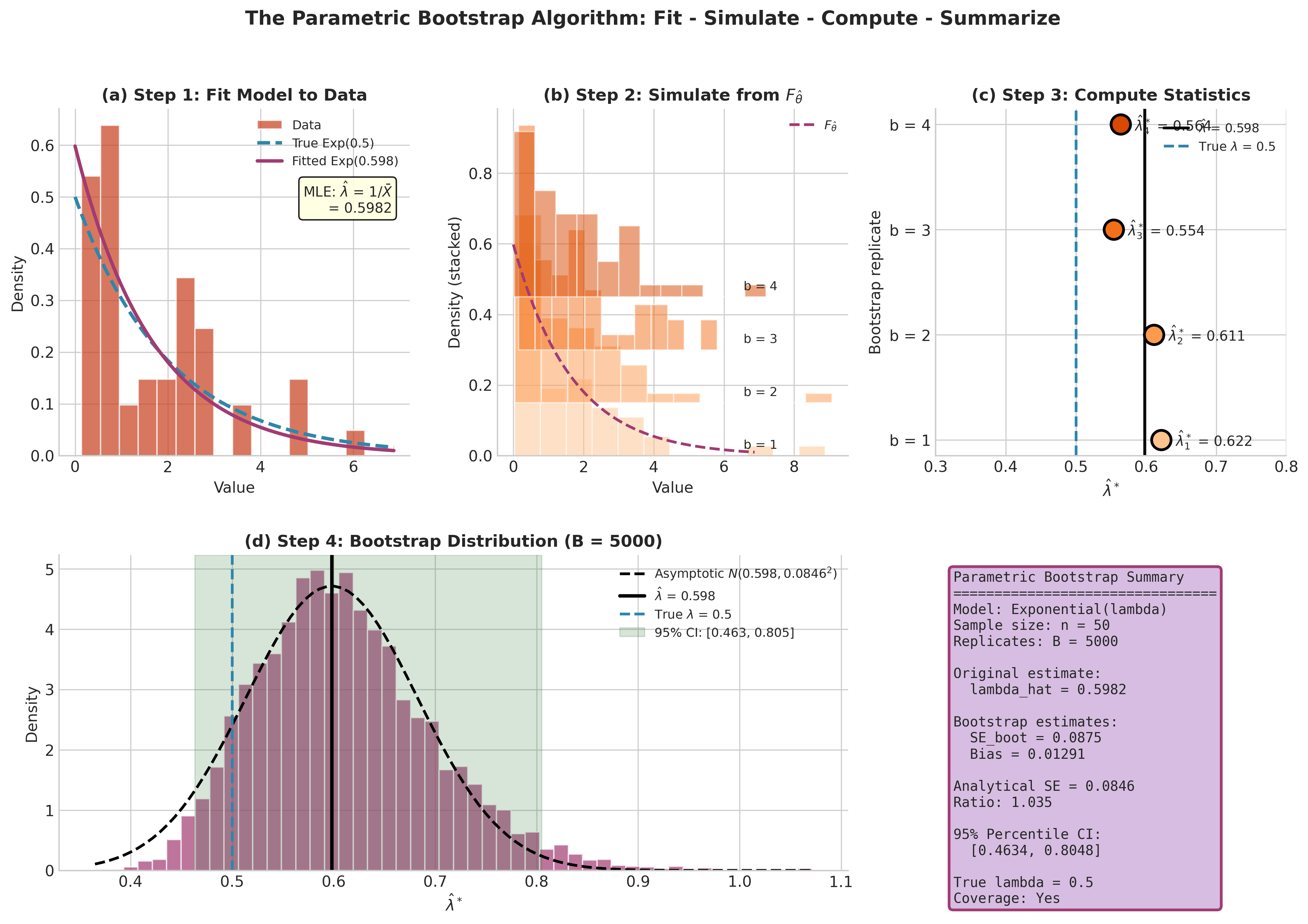
Fig. 153 Figure 4.4.2: The parametric bootstrap algorithm illustrated with exponential data. (a) Fit the model to data. (b) Simulate bootstrap samples from the fitted distribution. (c) Compute statistics on each sample. (d) Build the bootstrap distribution for inference.

Location-Scale Families

Many common distributions belong to location-scale families, where \(X = \mu + \sigma Z\) for standardized \(Z\). These include normal, Student-t, logistic, and Laplace distributions.

General Algorithm

Algorithm: Parametric Bootstrap for Location-Scale Families

Input: Data X₁, ..., Xₙ; location-scale family F; replicates B
Output: Bootstrap distribution of (μ̂*, σ̂*)

1. Estimate location μ̂ and scale σ̂ (MLE or robust estimators)
2. [Optional] Fit shape parameter if needed (e.g., df for t-distribution)
3. For b = 1, ..., B:
   a. Generate Z*₁, ..., Z*ₙ iid from the standard form of F
   b. Transform: X*ᵢ = μ̂ + σ̂ · Z*ᵢ
   c. Re-estimate (μ̂*, σ̂*) from X*
4. Return bootstrap estimates

Note: This is a pure parametric bootstrap—we simulate fresh standardized values from the assumed distribution, not from the empirical residuals. For a semi-parametric approach that resamples standardized residuals \(Z_i = (X_i - \hat{\mu})/\hat{\sigma}\), see the residual bootstrap in nonparametric-bootstrap.

Estimator Choices

The parametric bootstrap requires consistent estimators. Common choices:

Normal distribution:

• Location: \(\hat{\mu} = \bar{X}\) (MLE)

• Scale: \(\hat{\sigma} = s = \sqrt{\frac{1}{n-1}\sum(X_i - \bar{X})^2}\) (unbiased) or \(\hat{\sigma}_{MLE} = \sqrt{\frac{1}{n}\sum(X_i - \bar{X})^2}\)

Student-t distribution:

• Location: Sample mean or median

• Scale: \(\hat{\sigma} = s \cdot \sqrt{(\nu - 2)/\nu}\) for known \(\nu\)

• Degrees of freedom: Estimate via MLE or fix based on prior knowledge

Exponential/Gamma:

• Rate: \(\hat{\lambda} = 1/\bar{X}\) (MLE for exponential)

• Shape and rate: Method of moments or MLE for gamma

import numpy as np
from scipy import stats
from scipy.optimize import minimize_scalar

def bootstrap_location_scale(data, distribution='normal', B=2000, seed=None):
    """
    Parametric bootstrap for location-scale families.

    Parameters
    ----------
    data : array_like
        Sample data.
    distribution : str
        'normal', 't', 'laplace', or 'logistic'.
    B : int
        Number of bootstrap replicates.
    seed : int, optional
        Random seed.

    Returns
    -------
    dict with bootstrap results.
    """
    rng = np.random.default_rng(seed)
    data = np.asarray(data)
    n = len(data)

    # Fit distribution
    if distribution == 'normal':
        mu_hat, sigma_hat = data.mean(), data.std(ddof=1)
        rvs = lambda size: rng.normal(mu_hat, sigma_hat, size)
    elif distribution == 't':
        # Fit t-distribution via MLE
        df, loc, scale = stats.t.fit(data)
        mu_hat, sigma_hat = loc, scale
        rvs = lambda size: stats.t.rvs(df, loc=loc, scale=scale,
                                       size=size, random_state=rng)
    elif distribution == 'laplace':
        mu_hat = np.median(data)  # MLE for location
        sigma_hat = np.mean(np.abs(data - mu_hat))  # MLE for scale
        rvs = lambda size: rng.laplace(mu_hat, sigma_hat, size)
    elif distribution == 'logistic':
        mu_hat, sigma_hat = data.mean(), data.std() * np.sqrt(3) / np.pi
        rvs = lambda size: rng.logistic(mu_hat, sigma_hat, size)
    else:
        raise ValueError(f"Unknown distribution: {distribution}")

    # Bootstrap
    mu_star = np.empty(B)
    sigma_star = np.empty(B)

    for b in range(B):
        data_star = rvs(n)
        mu_star[b] = data_star.mean()
        sigma_star[b] = data_star.std(ddof=1)

    return {
        'mu_hat': mu_hat,
        'sigma_hat': sigma_hat,
        'mu_star': mu_star,
        'sigma_star': sigma_star,
        'se_mu': mu_star.std(ddof=1),
        'se_sigma': sigma_star.std(ddof=1),
        'ci_mu': np.quantile(mu_star, [0.025, 0.975]),
        'ci_sigma': np.quantile(sigma_star, [0.025, 0.975])
    }

Parametric Bootstrap for Regression

The parametric bootstrap for regression extends the residual bootstrap by assuming a distributional form for the errors rather than resampling observed residuals.

Fixed-X Parametric Bootstrap

For the linear model \(Y = X\beta + \varepsilon\) with \(\varepsilon \sim N(0, \sigma^2 I_n)\):

Algorithm: Parametric Bootstrap for OLS (Normal Errors)

Input: Design X (n × p), response Y, replicates B
Output: Bootstrap distribution of β̂*

1. Fit OLS: β̂ = (X'X)⁻¹X'Y
2. Compute residuals: ê = Y - Xβ̂
3. Estimate error variance: σ̂² = ||ê||² / (n - p)
4. For b = 1, ..., B:
   a. Generate ε*₁, ..., ε*ₙ iid ~ N(0, σ̂²)
   b. Form Y* = Xβ̂ + ε*
   c. Refit: β̂*_b = (X'X)⁻¹X'Y*
5. Return {β̂*₁, ..., β̂*_B}

Key insight: Unlike the residual bootstrap (which resamples \(\hat{e}_i\)), the parametric bootstrap draws fresh errors from \(N(0, \hat{\sigma}^2)\). This:

• Produces smooth bootstrap distributions

• Respects the assumed error structure

• Can be more efficient when normality holds

• Fails if errors are non-normal

Scope: Conditional Inference

This fixed-X parametric bootstrap targets conditional inference given X. If your predictors are random and you want unconditional inference on \(\beta\), you need a different resampling scheme (pairs bootstrap, or a generative model for X).

What is held fixed vs. resampled:

Component	Fixed-X Parametric	Pairs Bootstrap
Design matrix X	Fixed (same X in all replicates)	Resampled (rows of X change)
Error distribution	\(N(0, \hat{\sigma}^2)\) (assumed)	Empirical (from residuals)
Fitted means \(X\hat{\beta}\)	Fixed	Recomputed each replicate
Inference target	Conditional on X	Unconditional

Python Implementation

import numpy as np

def parametric_bootstrap_regression(X, y, B=2000, seed=None):
    """
    Parametric bootstrap for OLS regression with normal errors.

    Parameters
    ----------
    X : ndarray, shape (n, p)
        Design matrix (should include intercept column if desired).
    y : ndarray, shape (n,)
        Response vector.
    B : int
        Number of bootstrap replicates.
    seed : int, optional
        Random seed.

    Returns
    -------
    beta_star : ndarray, shape (B, p)
        Bootstrap distribution of coefficients.
    beta_hat : ndarray, shape (p,)
        OLS estimates.
    sigma_hat : float
        Estimated error standard deviation.
    """
    rng = np.random.default_rng(seed)
    X = np.asarray(X)
    y = np.asarray(y)
    n, p = X.shape

    # Fit OLS
    XtX_inv = np.linalg.inv(X.T @ X)
    beta_hat = XtX_inv @ X.T @ y
    y_hat = X @ beta_hat
    residuals = y - y_hat

    # Estimate error variance
    sigma_hat = np.sqrt(np.sum(residuals**2) / (n - p))

    # Parametric bootstrap
    beta_star = np.empty((B, p))

    for b in range(B):
        # Generate errors from N(0, σ̂²)
        eps_star = rng.normal(0, sigma_hat, size=n)
        y_star = y_hat + eps_star
        beta_star[b] = XtX_inv @ X.T @ y_star

    return beta_star, beta_hat, sigma_hat

Example 💡 Comparing Parametric and Nonparametric Bootstrap for Regression

Setup: Simulate data with normal errors and compare bootstrap approaches.

import numpy as np
import matplotlib.pyplot as plt

np.random.seed(42)

# Generate data with normal errors
n, p = 50, 2
X = np.column_stack([np.ones(n), np.random.uniform(-2, 2, n)])
beta_true = np.array([1.0, 2.0])
sigma_true = 0.5
y = X @ beta_true + np.random.normal(0, sigma_true, n)

B = 3000
rng = np.random.default_rng(123)

# Fit OLS
XtX_inv = np.linalg.inv(X.T @ X)
beta_hat = XtX_inv @ X.T @ y
y_hat = X @ beta_hat
residuals = y - y_hat
sigma_hat = np.sqrt(np.sum(residuals**2) / (n - p))

# Parametric bootstrap
beta_param = np.empty((B, p))
for b in range(B):
    eps_star = rng.normal(0, sigma_hat, size=n)
    y_star = y_hat + eps_star
    beta_param[b] = XtX_inv @ X.T @ y_star

# Nonparametric (residual) bootstrap
resid_centered = residuals - residuals.mean()
beta_nonparam = np.empty((B, p))
for b in range(B):
    idx = rng.integers(0, n, size=n)
    e_star = resid_centered[idx]
    y_star = y_hat + e_star
    beta_nonparam[b] = XtX_inv @ X.T @ y_star

# Compare
print("SE for β₁ (slope):")
print(f"  Parametric:    {beta_param[:, 1].std():.4f}")
print(f"  Nonparametric: {beta_nonparam[:, 1].std():.4f}")
print(f"  Analytical:    {sigma_hat * np.sqrt(XtX_inv[1,1]):.4f}")

Result: When errors are truly normal, all three approaches give similar SEs. The parametric bootstrap slightly outperforms when the model is correct.

Generalized Linear Models

For GLMs, the parametric bootstrap simulates from the fitted conditional distribution of \(Y | X\).

Algorithm: Parametric Bootstrap for GLM

Input: Design X, response Y, family (e.g., binomial, Poisson), replicates B
Output: Bootstrap distribution of β̂*

1. Fit GLM: β̂, compute μ̂ᵢ = g⁻¹(xᵢ'β̂) where g is the link function
2. For b = 1, ..., B:
   a. For each i, generate Y*ᵢ ~ Family(μ̂ᵢ, φ̂)
      - Binomial: Y*ᵢ ~ Binomial(nᵢ, μ̂ᵢ)
      - Poisson: Y*ᵢ ~ Poisson(μ̂ᵢ)
      - Gamma: Y*ᵢ ~ Gamma(α̂, μ̂ᵢ/α̂)
   b. Refit GLM on (X, Y*) to get β̂*_b
3. Return {β̂*₁, ..., β̂*_B}

import numpy as np
import statsmodels.api as sm

def parametric_bootstrap_glm(X, y, family, B=2000, seed=None, n_trials=None):
    """
    Parametric bootstrap for GLMs.

    Parameters
    ----------
    X : ndarray
        Design matrix (include intercept).
    y : ndarray
        Response.
    family : statsmodels family
        GLM family (e.g., sm.families.Poisson()).
    B : int
        Number of replicates.
    seed : int
        Random seed.
    n_trials : ndarray, optional
        Number of trials for Binomial family. Required if y contains
        counts > 1. If None and family is Binomial, assumes Bernoulli (n=1).

    Returns
    -------
    beta_star : ndarray, shape (B, p)
        Bootstrap coefficients.
    model : fitted GLM
        Original fitted model.
    """
    rng = np.random.default_rng(seed)

    # Fit original model
    model = sm.GLM(y, X, family=family).fit()
    beta_hat = model.params
    mu_hat = model.mu  # Fitted means

    p = len(beta_hat)
    beta_star = np.empty((B, p))

    # Check family type using class name (more robust than isinstance)
    family_name = family.__class__.__name__

    for b in range(B):
        # Generate from fitted distribution
        if family_name == 'Poisson':
            y_star = rng.poisson(mu_hat)

        elif family_name == 'Binomial':
            if n_trials is None:
                # Check if data looks like Bernoulli
                if np.all((y == 0) | (y == 1)):
                    n_trials = np.ones_like(y, dtype=int)
                else:
                    raise ValueError(
                        "n_trials required for Binomial with count data. "
                        "If y is binary (0/1), this is inferred automatically."
                    )
            y_star = rng.binomial(n_trials.astype(int), mu_hat)

        elif family_name == 'Gamma':
            # Gamma with shape from dispersion
            phi = model.scale
            shape = 1 / phi
            y_star = rng.gamma(shape, mu_hat / shape)

        else:
            raise NotImplementedError(f"Family {family_name} not implemented")

        # Refit
        try:
            model_star = sm.GLM(y_star, X, family=family).fit(disp=0)
            beta_star[b] = model_star.params
        except Exception:
            beta_star[b] = np.nan

    return beta_star, model

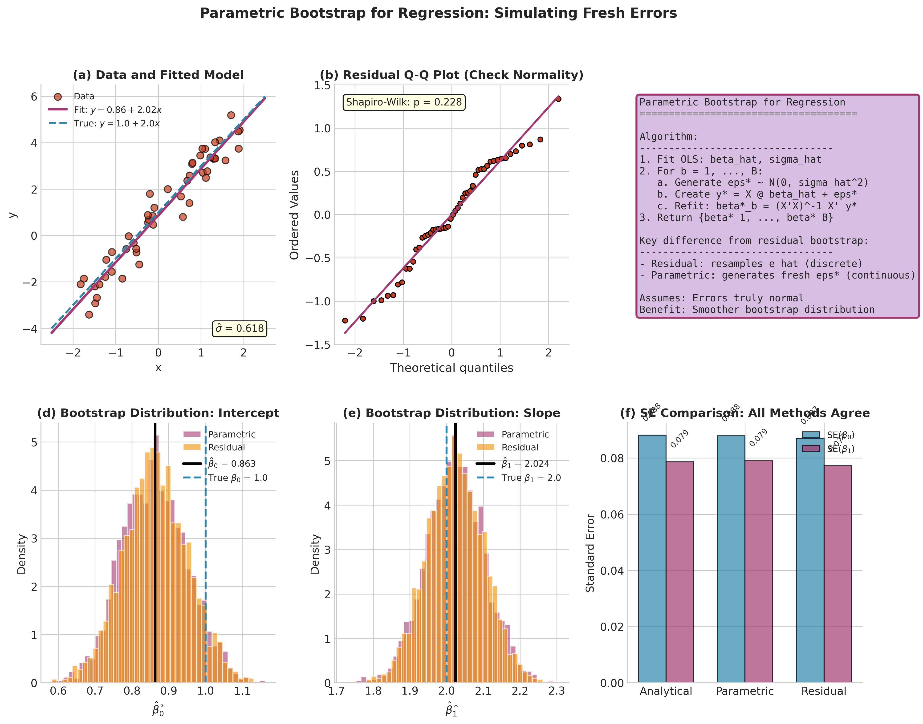
Fig. 154 Figure 4.4.5: Parametric bootstrap for regression. (a) Data and fitted model. (b) Q-Q plot to check normality assumption. (d-e) Bootstrap distributions for intercept and slope. (f) SE comparison shows agreement between analytical, parametric, and residual bootstrap when normality holds.

Confidence Intervals

Percentile Intervals

The simplest parametric bootstrap CI uses quantiles of the bootstrap distribution:

\[\text{CI}_{1-\alpha}^{\text{perc}} = \left[Q_{\alpha/2}(\hat{\theta}^*), Q_{1-\alpha/2}(\hat{\theta}^*)\right]\]

This is identical to nonparametric bootstrap percentile intervals in form, but the bootstrap distribution comes from parametric simulation.

Bootstrap-t (Studentized) Intervals

For second-order accuracy, use the studentized bootstrap:

1. For each bootstrap replicate, compute \(Z^*_b = (\hat{\theta}^*_b - \hat{\theta})/\hat{\text{SE}}^*_b\)

2. Find quantiles \(q_{\alpha/2}^*\) and \(q_{1-\alpha/2}^*\) of \(\{Z^*_b\}\)

3. CI: \([\hat{\theta} - q_{1-\alpha/2}^* \cdot \widehat{\text{SE}}, \hat{\theta} - q_{\alpha/2}^* \cdot \widehat{\text{SE}}]\)

\[\text{CI}_{1-\alpha}^{\text{boot-t}} = \left[\hat{\theta} - q^*_{1-\alpha/2} \cdot \widehat{\text{SE}}, \hat{\theta} - q^*_{\alpha/2} \cdot \widehat{\text{SE}}\right]\]

Advantage: Achieves \(O(n^{-1})\) coverage error versus \(O(n^{-1/2})\) for percentile intervals.

Disadvantage: Requires estimating SE within each bootstrap replicate (nested bootstrap or analytical formula).

BCa Intervals with Parametric Bootstrap

The BCa method (Bias-Corrected and accelerated) can be applied to parametric bootstrap as well:

\[z_0 = \Phi^{-1}\left(\frac{\#\{\hat{\theta}^*_b < \hat{\theta}\}}{B}\right), \quad \hat{a} = \frac{\sum_{i=1}^n (\bar{\theta}_{(\cdot)} - \hat{\theta}_{(-i)})^3}{6\left[\sum_{i=1}^n (\bar{\theta}_{(\cdot)} - \hat{\theta}_{(-i)})^2\right]^{3/2}}\]

The adjusted quantiles are:

\[\alpha_1 = \Phi\left(z_0 + \frac{z_0 + z_{\alpha/2}}{1 - \hat{a}(z_0 + z_{\alpha/2})}\right), \quad \alpha_2 = \Phi\left(z_0 + \frac{z_0 + z_{1-\alpha/2}}{1 - \hat{a}(z_0 + z_{1-\alpha/2})}\right)\]

BCa intervals are transformation-invariant and range-preserving, making them excellent for parameters with natural bounds.

Python Implementation of CI Methods

import numpy as np
from scipy import stats

def parametric_bootstrap_ci(theta_star, theta_hat, alpha=0.05,
                             method='percentile', se_hat=None,
                             se_star=None, theta_jack=None):
    """
    Confidence intervals from parametric bootstrap.

    Parameters
    ----------
    theta_star : ndarray
        Bootstrap replicates.
    theta_hat : float
        Original estimate.
    alpha : float
        Significance level.
    method : str
        'percentile', 'basic', 'normal', 'studentized', or 'bca'.
    se_hat : float, optional
        SE estimate for original data (needed for 'normal', 'studentized').
    se_star : ndarray, optional
        Per-replicate SE estimates (needed for true 'studentized').
        If None with 'studentized', falls back to pseudo-studentized.
    theta_jack : ndarray, optional
        Jackknife estimates (needed for 'bca').

    Returns
    -------
    ci : tuple
        (lower, upper) confidence limits.
    """
    B = len(theta_star)

    if method == 'percentile':
        return (np.quantile(theta_star, alpha/2),
                np.quantile(theta_star, 1 - alpha/2))

    elif method == 'basic':
        q_lo = np.quantile(theta_star, alpha/2)
        q_hi = np.quantile(theta_star, 1 - alpha/2)
        return (2*theta_hat - q_hi, 2*theta_hat - q_lo)

    elif method == 'normal':
        if se_hat is None:
            se_hat = theta_star.std(ddof=1)
        z = stats.norm.ppf(1 - alpha/2)
        return (theta_hat - z*se_hat, theta_hat + z*se_hat)

    elif method == 'studentized':
        # True studentized bootstrap requires SE for each replicate
        if se_hat is None:
            raise ValueError("se_hat required for studentized method")

        if se_star is not None:
            # Proper studentized bootstrap with per-replicate SEs
            t_star = (theta_star - theta_hat) / se_star
        else:
            # Pseudo-studentized: uses single SE (does NOT achieve
            # second-order accuracy; use only as approximation)
            import warnings
            warnings.warn("se_star not provided; using pseudo-studentized "
                        "method which does not achieve second-order accuracy")
            t_star = (theta_star - theta_hat) / se_hat

        q_lo = np.quantile(t_star, alpha/2)
        q_hi = np.quantile(t_star, 1 - alpha/2)
        return (theta_hat - q_hi*se_hat, theta_hat - q_lo*se_hat)

    elif method == 'bca':
        if theta_jack is None:
            raise ValueError("Jackknife estimates required for BCa")

        # Bias correction
        prop_below = np.mean(theta_star < theta_hat)
        z0 = stats.norm.ppf(prop_below) if 0 < prop_below < 1 else 0

        # Acceleration
        theta_bar = theta_jack.mean()
        num = np.sum((theta_bar - theta_jack)**3)
        denom = 6 * np.sum((theta_bar - theta_jack)**2)**1.5
        a_hat = num / denom if denom != 0 else 0

        # Adjusted quantiles
        z_alpha = stats.norm.ppf(alpha/2)
        z_1alpha = stats.norm.ppf(1 - alpha/2)

        def adj_quantile(z):
            return stats.norm.cdf(z0 + (z0 + z)/(1 - a_hat*(z0 + z)))

        alpha1 = adj_quantile(z_alpha)
        alpha2 = adj_quantile(z_1alpha)

        return (np.quantile(theta_star, alpha1),
                np.quantile(theta_star, alpha2))

    else:
        raise ValueError(f"Unknown method: {method}")

Model Checking and Validation

The parametric bootstrap’s validity depends critically on model correctness. Before relying on parametric bootstrap, verify assumptions.

Diagnostic Checks

1. Graphical diagnostics:

   • Q-Q plot of residuals against assumed distribution

   • Residual plots for heteroscedasticity

   • Scale-location plot for variance stability

2. Formal tests (use with caution—low power for small \(n\)):

   • Shapiro-Wilk for normality

   • Breusch-Pagan for heteroscedasticity

   • Anderson-Darling for distributional fit

3. Sensitivity analysis:

   • Compare parametric and nonparametric bootstrap CIs

   • If they differ substantially, investigate model assumptions

import numpy as np
import matplotlib.pyplot as plt
from scipy import stats

def check_parametric_assumptions(residuals, distribution='normal'):
    """
    Diagnostic plots for parametric bootstrap assumptions.

    Parameters
    ----------
    residuals : array_like
        Model residuals.
    distribution : str
        Assumed distribution ('normal', 't', etc.).
    """
    residuals = np.asarray(residuals)
    n = len(residuals)

    fig, axes = plt.subplots(2, 2, figsize=(10, 8))

    # Q-Q plot
    ax = axes[0, 0]
    if distribution == 'normal':
        stats.probplot(residuals, dist="norm", plot=ax)
    elif distribution == 't':
        # Fit df, then Q-Q
        df = stats.t.fit(residuals)[0]
        stats.probplot(residuals, dist=stats.t(df), plot=ax)
    ax.set_title('Q-Q Plot')

    # Histogram with fitted distribution
    ax = axes[0, 1]
    ax.hist(residuals, bins='auto', density=True, alpha=0.7,
            edgecolor='black')
    x = np.linspace(residuals.min(), residuals.max(), 100)
    if distribution == 'normal':
        mu, sigma = residuals.mean(), residuals.std()
        ax.plot(x, stats.norm.pdf(x, mu, sigma), 'r-', lw=2,
                label='Fitted Normal')
    ax.legend()
    ax.set_title('Histogram vs Fitted Distribution')

    # Residuals vs fitted (check for patterns)
    ax = axes[1, 0]
    ax.scatter(np.arange(n), residuals, alpha=0.5)
    ax.axhline(0, color='red', linestyle='--')
    ax.set_xlabel('Index')
    ax.set_ylabel('Residuals')
    ax.set_title('Residuals vs Index')

    # Scale-location plot
    ax = axes[1, 1]
    std_resid = residuals / residuals.std()
    ax.scatter(np.arange(n), np.sqrt(np.abs(std_resid)), alpha=0.5)
    ax.set_xlabel('Index')
    ax.set_ylabel('√|Standardized Residuals|')
    ax.set_title('Scale-Location Plot')

    plt.tight_layout()

    # Formal tests
    print("Diagnostic Tests:")
    if distribution == 'normal':
        stat, p = stats.shapiro(residuals)
        print(f"  Shapiro-Wilk: W={stat:.4f}, p={p:.4f}")

    # Runs test for independence
    median = np.median(residuals)
    signs = residuals > median
    runs = 1 + np.sum(signs[1:] != signs[:-1])
    n_pos, n_neg = signs.sum(), (~signs).sum()
    exp_runs = 1 + 2*n_pos*n_neg / n
    var_runs = 2*n_pos*n_neg*(2*n_pos*n_neg - n) / (n**2 * (n-1))
    z_runs = (runs - exp_runs) / np.sqrt(var_runs)
    print(f"  Runs test: z={z_runs:.4f}, p={2*(1-stats.norm.cdf(abs(z_runs))):.4f}")

    return fig

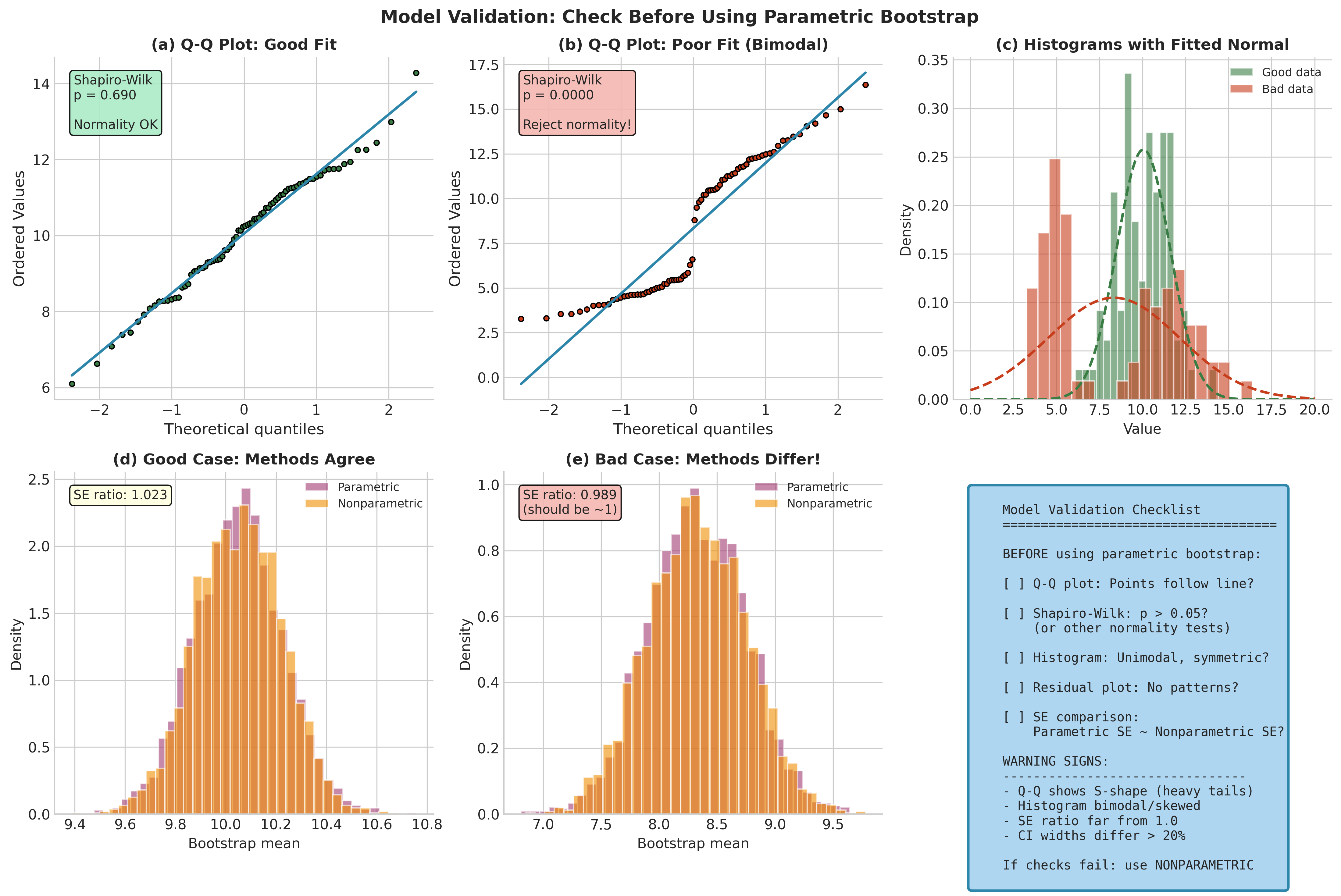
Fig. 155 Figure 4.4.7: Model validation diagnostics. Left column shows a well-behaved case (normal data) where parametric assumptions hold. Right column shows a problematic case (bimodal data) where normality fails. When methods disagree (panel e), investigate model assumptions.

Common Pitfall ⚠️

Trusting the wrong model: If you use parametric bootstrap with a misspecified model (e.g., assuming normality when errors are heavy-tailed), confidence intervals may have severely incorrect coverage. Always validate assumptions before relying on parametric bootstrap.

Course heuristic: If parametric and nonparametric bootstrap CIs differ by more than 20% in width, this is a flag to investigate model assumptions carefully. This threshold is not a formal statistical rule but a practical signal that something may warrant attention.

When Parametric Bootstrap Fails

Model Misspecification

The most serious parametric-bootstrap failure mode is model misspecification. If the true distribution \(F\) is meaningfully outside the assumed family \(\{F_\theta\}\), then simulating from \(F_{\hat\theta}\) does not reproduce the sampling behavior of the statistic under the real data-generating process. In that case, the parametric bootstrap can deliver biased standard errors and confidence intervals with severe undercoverage.

A particularly fragile setting is inference for a tail functional, such as \(p = \Pr(X > c)\), because \(p\) depends on the distribution’s extreme-right behavior. In the example below, the true distribution is a mixture (bimodal). Fitting a single Normal forces the model to “average” the two modes, which misrepresents the right tail that determines \(p\).

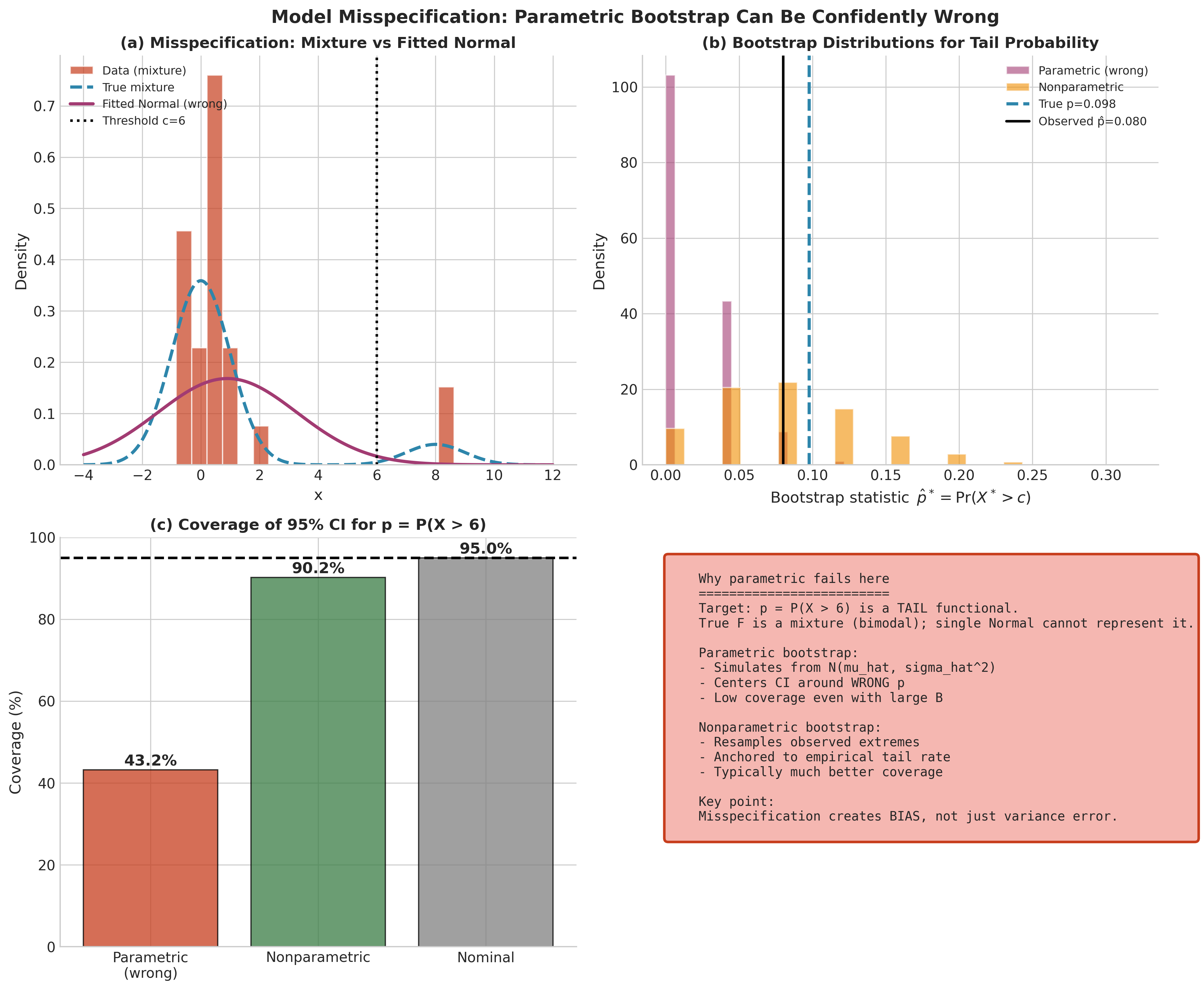
Fig. 156 Figure 4.4.4: Model misspecification, parametric bootstrap can be confidently wrong. (a) Data are generated from a mixture distribution, but a single Normal model is fitted, producing a tail mismatch beyond the threshold \(c=6\). (b) Bootstrap distributions for \(\hat{p}^* = \Pr(X^* > c)\) differ sharply: the parametric bootstrap (wrong model) concentrates on smaller values, while the nonparametric bootstrap remains anchored to the empirical tail behavior. (c) In repeated-sampling experiments, the 95% parametric-bootstrap CI for \(p\) can have drastic undercoverage under misspecification, whereas the nonparametric bootstrap is typically much closer to nominal.

Boundary Parameters

Boundary and near boundary settings are nonregular: the estimator’s sampling distribution can be highly asymmetric, and the usual bootstrap logic can break. In these cases, the parametric bootstrap can fail, and the standard nonparametric bootstrap can fail as well when the statistic is constrained by the sample support.

• Uniform[0, (theta)] (endpoint / maximum): If \(\hat{\theta} = X_{(n)}\) (the sample maximum), then a parametric bootstrap that simulates \(X^* \sim \mathrm{Unif}(0,\hat{\theta})\) produces \(\hat{\theta}^*=\max(X^*) \le \hat{\theta}\) always. This truncation makes it impossible to represent upward uncertainty in \(\theta\). The same structural problem occurs for the standard nonparametric bootstrap, since resampling from \(\hat F_n\) cannot generate observations exceeding \(X_{(n)}\).

• Variance near 0 (degenerate scale estimate): If the sample variance is extremely small, a parametric bootstrap from \(N(\hat{\mu},\hat{\sigma}^2)\) with tiny \(\hat{\sigma}\) yields nearly degenerate bootstrap samples and misleadingly small standard errors.

Remedies (choose based on context): - Exact finite-sample theory when available: for Uniform endpoints, order-statistic results yield exact tail probabilities and CIs. - Bias-corrected or alternative estimators: for Uniform[0, (theta)],

\(\hat{\theta}_{bc}=\frac{n+1}{n}X_{(n)}\) removes the downward bias in \(X_{(n)}\).

• Subsampling / m-out-of-n bootstrap: resample \(m<n\) observations (with or without replacement) to obtain a distributional approximation that is often more stable in nonregular settings.

• Reparameterization: when possible, transform to an unconstrained scale to avoid boundary artifacts.

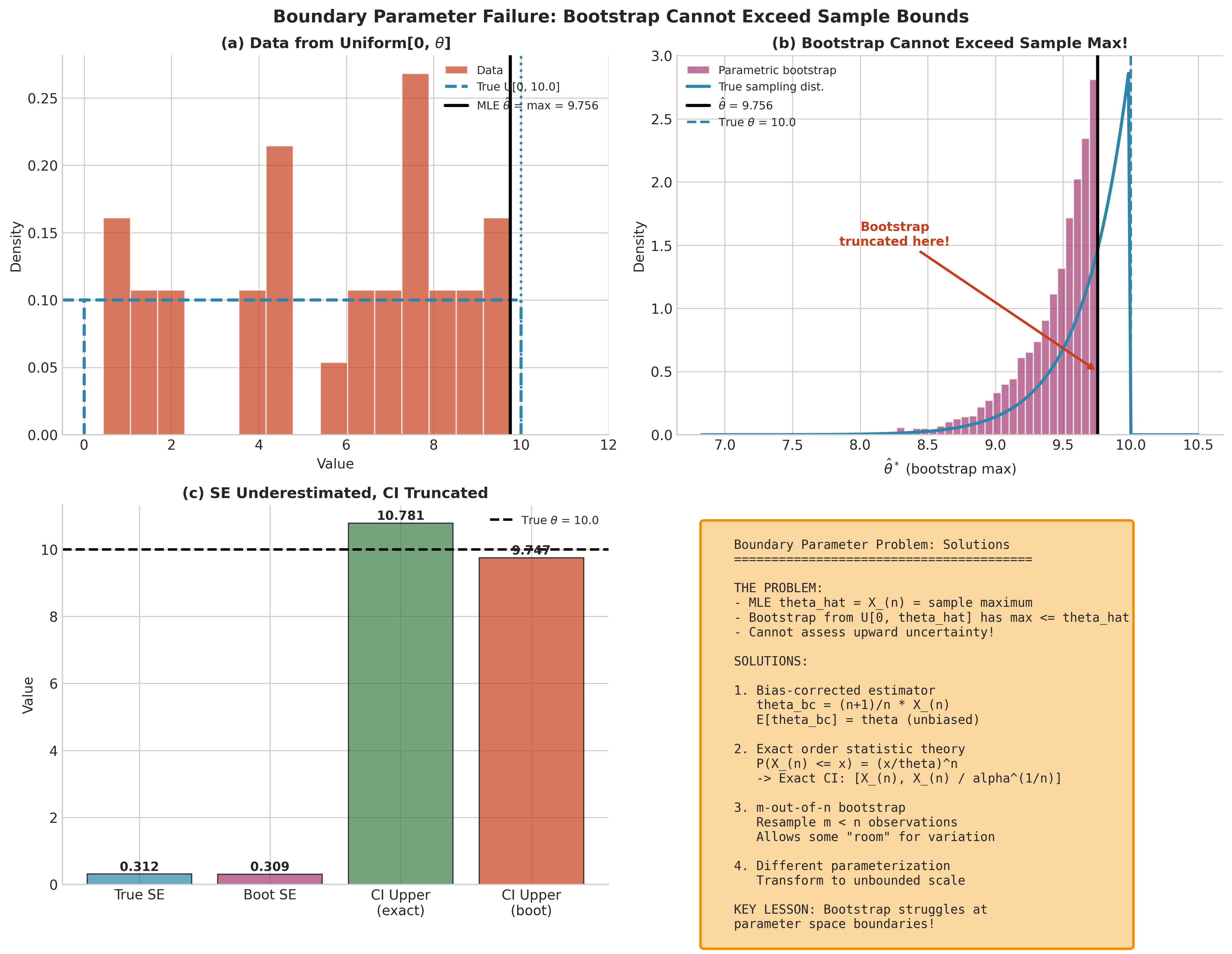
Fig. 157 Figure 4.4.6: Boundary parameter failure for Uniform[0, \(\theta\)]. (a) The MLE \(\hat{\theta}=X_{(n)}\) typically underestimates the true endpoint. (b) Parametric bootstrap from \(\mathrm{Unif}(0,\hat{\theta})\) is truncated at \(\hat{\theta}\) (and the standard nonparametric bootstrap is similarly truncated), so upward uncertainty cannot be represented. (c) The resulting bootstrap standard error and percentile CI upper bound are biased downward relative to the true sampling behavior.

Heavy-Tailed Distributions

Heavy tails can break bootstrap inference, but the issue depends on both the tail behavior of \(F\) and the statistic \(T_n\).

• If \(F\) has infinite variance (e.g., stable laws with \(\alpha < 2\)), then the sample mean and other non-robust, variance-dependent functionals often have nonstandard asymptotics (no CLT, stable limits, or extremely slow convergence). In these regimes, the usual nonparametric bootstrap may give a poor or even inconsistent approximation to the sampling distribution of \(T_n\).

• In the extreme case of no finite mean (e.g., Cauchy), the sample mean does not stabilize in the usual sense; it does not concentrate around a constant. A bootstrap distribution built from \(\hat F_n\) cannot recover a “nice” sampling law for \(\bar X\) because the target itself is nonstandard.

Robust statistics are typically safer under heavy tails. Medians, trimmed means, and many M-estimators can retain well-behaved limiting distributions (often asymptotically normal under mild conditions) and are therefore more compatible with bootstrap inference.

Remedy: Prefer robust estimators (median, trimmed mean, appropriate M-estimators), and choose a bootstrap that matches the estimator and tail regime. When tails are very heavy, consider diagnostics (tail plots, extreme values) and sensitivity checks across multiple robust choices.

Parametric vs. Nonparametric: A Decision Framework

Choosing between parametric and nonparametric bootstrap involves balancing efficiency against robustness.

Table 47 Parametric vs. Nonparametric Bootstrap

Criterion	Parametric Bootstrap	Nonparametric Bootstrap
Primary assumption	Data follow a specified family \(\{F_\theta\}\) (after fitting \(\hat\theta\))	Uses \(\hat F_n\); fewer distributional assumptions
When it shines	Often more efficient when the model is credible, especially for small \(n\)	Generally more robust to distributional misspecification
Small samples (\(n \lesssim 30\))	Can give tighter, more stable inference if the model is correct	Can be noisier (discrete resampling, higher Monte Carlo variability), but often still reasonable
Model misspecification	Can fail badly (bias, undercoverage, misleading SEs)	Typically more robust, but not universally “always valid”
Complex statistics / functionals	Often straightforward (simulate from fitted model, recompute statistic)	Often straightforward (resample data, recompute statistic)
Support constraints / boundaries	Can fail for boundary MLEs (e.g., \(\hat\theta = X_{(n)}\)); may require special remedies	Can also fail or be conservative for extreme order statistics; may require m-out-of-n / subsampling
Computational cost	Usually \(O(Bn)\) plus model fitting if refit each replicate	Usually \(O(Bn)\) plus any refitting inside each replicate

Decision Flowchart

1. Do you have strong prior knowledge for a parametric family?

   • No → Start with nonparametric.

   • Yes → Continue.

2. Do basic diagnostics support the model (shape, tails, support)?

   • Clear departures (skewness, multimodality, heavy tails, truncation) → Prefer nonparametric or revise the model.

   • Diagnostics look reasonable → Continue.

3. Is the sample size small (:math:`n lesssim 30`)?

   • Yes and model credible → Parametric often improves efficiency and stability.

   • Yes and model uncertain → Prefer nonparametric, and treat parametric as a sensitivity check only.

4. Is the target sensitive to tails or support (extremes, thresholds, quantiles)?

   • Yes → Parametric assumptions matter more; validate aggressively and consider robust or tail-appropriate models.

   • No → Either method may work; compare as a robustness check.

5. When in doubt: Run both. If results differ materially, diagnose why (model fit, tails, boundaries, dependence).

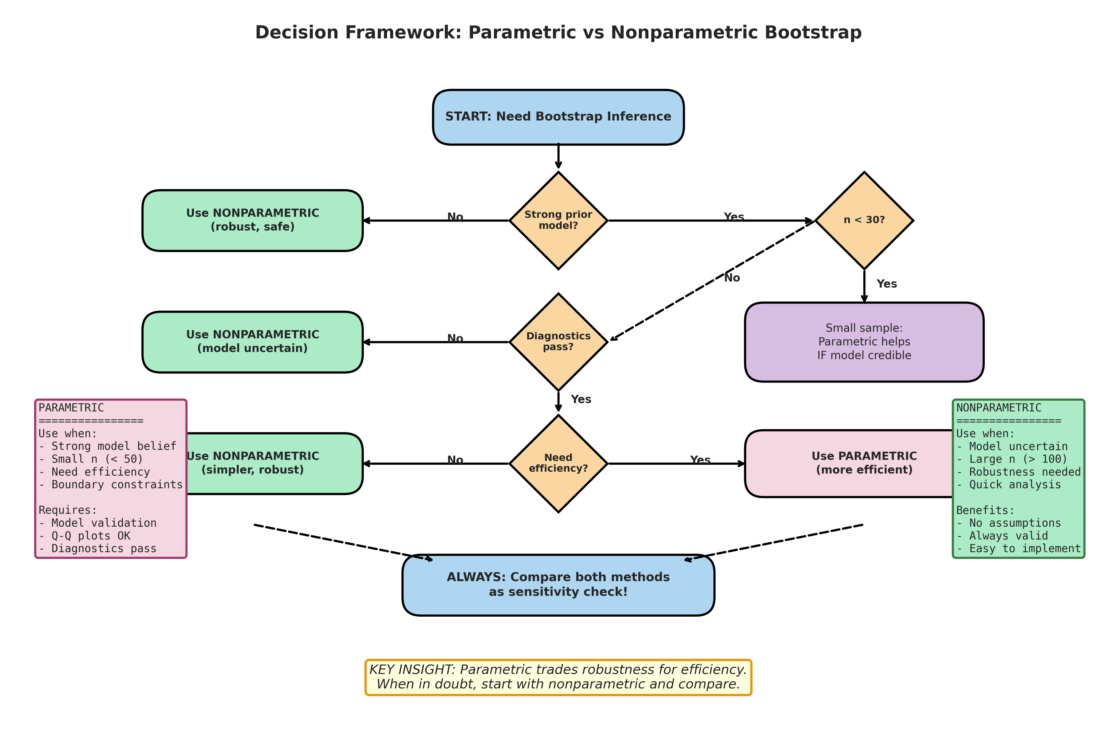
Fig. 158 Figure 4.4.8: Decision framework for choosing between parametric and nonparametric bootstrap. Parametric bootstrap trades robustness for efficiency. A practical default is to start with nonparametric and use parametric only when the model is credible and diagnostics support it.

Practical Recommendation

Default: Start with nonparametric for robustness, then compare with a parametric bootstrap if a credible model exists.

Prefer parametric bootstrap when:

1. You have a well-justified parametric family for \(F\)

2. Diagnostics do not show clear shape or tail conflicts

3. \(n\) is small and efficiency matters

Use special remedies near boundaries or extremes (for either method):

• Exact theory when available (order statistics, known pivots)

• Bias-corrected estimators (e.g., \(\hat\theta_{bc} = \frac{n+1}{n} X_{(n)}\))

• m-out-of-n bootstrap or subsampling for boundary or extreme-value functionals

Practical Considerations

Computational Efficiency

• Vectorization: Pre-generate all \(B \times n\) random values at once, then reshape

# Instead of loop:
# for b in range(B):
#     eps = rng.normal(0, sigma, n)

# Vectorized:
eps_all = rng.normal(0, sigma, size=(B, n))
# Then process all B samples simultaneously

• Parallel computation: Bootstrap replicates are independent; parallelize across cores

• Analytical shortcuts: For some parametric families, bootstrap distributions have closed forms (e.g., normal mean bootstrap is exactly \(N(\hat{\mu}, \hat{\sigma}^2/n)\))

Choosing B

Recommendations mirror nonparametric bootstrap:

• SE estimation: \(B = 500\) to \(2{,}000\)

• Confidence intervals: \(B = 2{,}000\) to \(10{,}000\)

• P-values: \(B \geq 10{,}000\) for \(\alpha = 0.05\)

Monte Carlo error decreases as \(O(1/\sqrt{B})\), so doubling precision requires quadrupling \(B\).

Reporting Standards

A parametric bootstrap analysis should report:

1. The assumed model: Distribution family and any fixed parameters

2. Estimation method: MLE, method of moments, etc.

3. Model diagnostics: Evidence supporting distributional assumptions

4. Bootstrap details: Number of replicates \(B\), random seed

5. CI method: Percentile, bootstrap-t, BCa

6. Comparison (recommended): Results from nonparametric bootstrap as sensitivity check

Bringing It All Together

The parametric bootstrap is a powerful tool when model assumptions are credible. It offers improved efficiency and finite-sample performance compared to nonparametric approaches, particularly for small samples and well-understood parametric families. The key tradeoff is robustness: parametric bootstrap can fail badly under model misspecification.

The decision between parametric and nonparametric bootstrap should be guided by:

• Prior knowledge about the data-generating process

• Sample size and the stakes of the analysis

• Diagnostic evidence for model fit

• Sensitivity of conclusions to method choice

Key Takeaways 📝

1. Core concept: Parametric bootstrap simulates from a fitted parametric model \(F_{\hat{\theta}}\) rather than resampling from the empirical distribution \(\hat{F}_n\).

2. Efficiency-robustness tradeoff: Parametric bootstrap is more efficient when the model is correct, but fails under misspecification; nonparametric bootstrap is robust but less efficient.

3. When to use parametric: Small samples with credible models, well-established parametric families, when efficiency matters, or when nonparametric methods encounter boundary issues.

4. Critical requirement: Always validate model assumptions through diagnostic plots and, when possible, compare to nonparametric results.

5. Outcome alignment: This section addresses LO 1 (simulation techniques) and LO 3 (resampling for CIs and variability assessment).

References

Primary Sources

[Efron1979]

Efron, B. (1979). Bootstrap methods: Another look at the jackknife. The Annals of Statistics, 7(1), 1–26. The original bootstrap paper, introducing resampling from the ECDF as the foundation for all bootstrap methods.

[EfronTibshirani1993]

Efron, B., and Tibshirani, R. J. (1993). An Introduction to the Bootstrap. Chapman & Hall/CRC. The definitive textbook on bootstrap methods, including comprehensive coverage of parametric approaches.

[DavisonHinkley1997]

Davison, A. C., and Hinkley, D. V. (1997). Bootstrap Methods and Their Application. Cambridge University Press. Comprehensive treatment with extensive coverage of parametric bootstrap, regression methods, and practical applications.

Theoretical Foundations

[Hall1992]

Hall, P. (1992). The Bootstrap and Edgeworth Expansion. Springer. Mathematical foundations of higher-order accuracy and studentization theory underlying bootstrap confidence intervals.

[Beran1997]

Beran, R. (1997). Diagnosing bootstrap success. Annals of the Institute of Statistical Mathematics, 49(1), 1–24. Conditions for bootstrap consistency and systematic treatment of failure modes.

[ShaoTu1995]

Shao, J., and Tu, D. (1995). The Jackknife and Bootstrap. Springer. Unified mathematical treatment of resampling methods with rigorous proofs of consistency.

Regression Bootstrap

[Freedman1981]

Freedman, D. A. (1981). Bootstrapping regression models. The Annals of Statistics, 9(6), 1218–1228. Foundational paper comparing pairs and residual bootstrap approaches for linear models.

[Wu1986]

Wu, C. F. J. (1986). Jackknife, bootstrap and other resampling methods in regression analysis. The Annals of Statistics, 14(4), 1261–1295. Introduction of the wild bootstrap for heteroscedasticity with fixed design matrices.

Confidence Interval Methods

[Efron1987]

Efron, B. (1987). Better bootstrap confidence intervals. Journal of the American Statistical Association, 82(397), 171–185. Introduction of the bias-corrected and accelerated (BCa) interval method.

[DiCiccioEfron1996]

DiCiccio, T. J., and Efron, B. (1996). Bootstrap confidence intervals. Statistical Science, 11(3), 189–228. Comprehensive review of percentile, studentized, basic, and BCa confidence interval methods.

Computational

[CantyRipley]

Canty, A., and Ripley, B. D. boot: Bootstrap R (S-Plus) Functions. R package. https://CRAN.R-project.org/package=boot. Standard R implementation of bootstrap methods; version numbers update regularly.