Section 5.6 Probabilistic Programming with PyMC

Sections 5.4 and 5.5 established the mathematical foundations of MCMC and implemented Metropolis-Hastings and Gibbs sampling from scratch. Those implementations were deliberately explicit: every acceptance step, every log-density evaluation, every pre-allocated random array was visible. The pedagogical purpose was to make the machinery comprehensible. The practical reality is that no applied Bayesian analysis uses hand-coded MCMC — it uses probabilistic programming languages (PPLs), which automate the construction, optimisation, and sampling of posterior distributions from a compact model specification.

PyMC is the leading Python PPL for applied Bayesian statistics, combining expressive model syntax, state-of-the-art NUTS sampling, and the ArviZ ecosystem for diagnostics and visualisation. The PyMC 5 blocks in Section 5.2 Prior Specification and Conjugate Analysis introduced the workflow on simple conjugate models, where the MCMC machinery was almost invisible because the posteriors were so tractable. This section develops the full workflow on non-conjugate models — logistic regression and Poisson regression — where PyMC’s automation is genuinely necessary and its diagnostic output demands serious attention.

By the end of this section, you will be able to specify, sample, diagnose, and interpret any single-level Bayesian model in PyMC. The more complex hierarchical structure is deferred to Section 5.8 Hierarchical Models and Partial Pooling (Optional); the model comparison methods that consume this section’s MCMC output are developed in Section 5.7 Bayesian Model Comparison.

Road Map 🧭

• Understand: How PyMC converts a model specification into a computation graph and uses automatic differentiation to run NUTS without user-supplied gradients

• Develop: Facility with the full PyMC workflow — prior specification, sampling, InferenceData structure, diagnostic plots, and posterior predictive checks

• Implement: Logistic and Poisson regression models in PyMC with proper priors, convergence verification, and out-of-sample prediction

• Evaluate: Chain convergence and model adequacy using az.summary, az.plot_trace, az.plot_pair, and posterior predictive checks

How PyMC Works: From Model Spec to Gradient

Understanding what happens when you run pm.sample() — rather than treating it as a black box — is what separates a practitioner who can diagnose failures from one who cannot.

The Computation Graph

When you write a PyMC model inside a with pm.Model() block, you are not computing anything yet. You are constructing a computation graph — a directed acyclic graph (DAG: a network of nodes connected by directed edges with no cycles, so information flows in one direction only) in which each node represents either a random variable or a deterministic transformation, and each edge represents a dependency. PyMC builds this graph using the Pytensor library, which represents mathematical expressions symbolically in the same way that a computer algebra system would.

Consider a simple regression model. Writing beta = pm.Normal('beta', mu=0, sigma=2.5) creates a symbolic node representing a Normal random variable; it does not draw a number. Writing mu = pm.Deterministic('mu', alpha + beta * x) creates a deterministic node that transforms the symbolic alpha and beta through a linear combination. Writing y = pm.Normal('y', mu=mu, sigma=sigma, observed=y_obs) pins the observed data to the likelihood node. The entire model — prior, likelihood, and any derived quantities — becomes a single symbolic expression.

From this graph, Pytensor can compute the log-posterior \(\log p(\theta \mid y)\) and, crucially, its gradient \(\nabla_\theta \log p(\theta \mid y)\) by applying the chain rule symbolically through the graph. This is what automatic differentiation (introduced in Section 5.5 MCMC Algorithms: Metropolis-Hastings and Gibbs Sampling) means in practice: the gradient is computed exactly, not approximated, and the user never writes a single derivative by hand. Every distribution node contributes its log-density; every deterministic node contributes via the chain rule; the result is an exact gradient function compiled to machine code before sampling begins.

From Graph to NUTS

Once the computation graph exists, pm.sample() does the following:

1. Initialise: Find a starting point with reasonable log-density, either from ADVI (Automatic Differentiation Variational Inference — a fast approximate method that fits a simple distribution, typically a diagonal Normal, to the posterior by minimising a divergence measure; it runs in seconds and provides a starting point and rough scale estimate for the chain) or from user-supplied values.

2. Warm-up: Run NUTS for the specified number of warm-up steps, adapting the step size \(\epsilon\) and mass matrix \(M\) (introduced in Section 5.4 Markov Chains: The Mathematical Foundation of MCMC) using dual averaging — an adaptive scheme that targets a user-specified acceptance rate (target_accept) by automatically adjusting \(\epsilon\) so the empirical acceptance rate converges to the target. The default target_accept=0.80 is appropriate for most models; increasing it toward 0.95 forces smaller step sizes and is the first remedy for divergences.

3. Sample: Run NUTS for the specified number of draws, holding \(\epsilon\) and \(M\) fixed at the tuned values.

4. Store: Package all samples, log-densities, acceptance rates, and tree statistics into an InferenceData object.

This is what Section 5.5 MCMC Algorithms: Metropolis-Hastings and Gibbs Sampling described abstractly as “PyMC compiles the model to a computation graph with automatic differentiation, runs NUTS for continuous parameters, handles warm-up and adaptation automatically.” Now you know concretely what each step involves.

The InferenceData Object

pm.sample() returns an ArviZ InferenceData object — a structured container that organises all outputs of a Bayesian analysis. Its main components are:

• idata.posterior: An xarray.Dataset — a labelled multi-dimensional array container (think of it as a dictionary of NumPy arrays, each with named dimensions) — with dimensions (chain, draw, *param_dims). This is where the MCMC samples live. To get a flat NumPy array for a scalar parameter theta, use idata.posterior['theta'].values.flatten().

• idata.sample_stats: Sampler diagnostics per draw — acceptance probability, tree depth, divergences, step size. Divergences (idata.sample_stats['diverging']) are a critical diagnostic: even one divergence in a converged chain signals that the sampler encountered a region of the posterior it could not traverse, and posterior summaries near that region may be unreliable.

• idata.posterior_predictive: Populated after calling pm.sample_posterior_predictive. Contains simulated observations drawn from the likelihood at each posterior sample — the raw material for posterior predictive checks.

• idata.observed_data: The observed data, stored for reference.

• idata.log_likelihood: Per-observation log-likelihoods, computed if pm.compute_log_likelihood(idata) is called. Required for model comparison via WAIC and LOO (Section 5.7 Bayesian Model Comparison).

Common Pitfall ⚠️

Divergences are not warnings — they are errors. A divergence occurs when the leapfrog integrator encounters a region of extreme posterior curvature and the numerical trajectory goes unstable. Even a single divergence in thousands of draws can bias posterior estimates in the region where the divergence occurred. The correct response to divergences is not to increase the number of draws but to reparameterise the model — typically switching to a non-centred parameterisation for hierarchical models (see Section 5.8 Hierarchical Models and Partial Pooling (Optional)) — or to increase target_accept to force smaller step sizes. Never report results from a model with unresolved divergences.

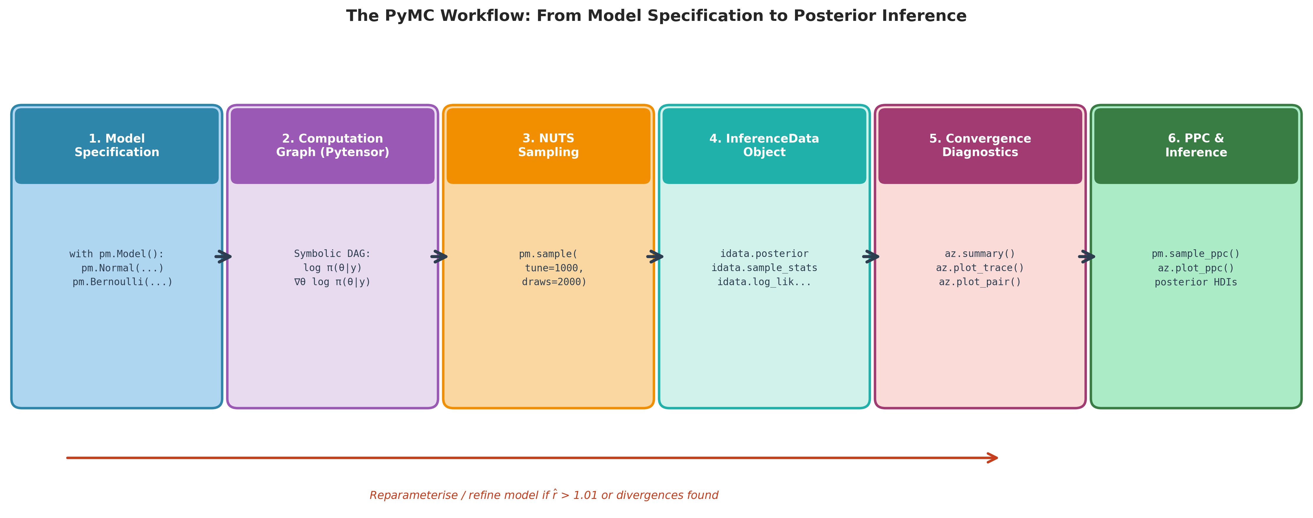
Fig. 199 Figure 5.28. The PyMC workflow. Each stage is automated by PyMC or ArviZ and corresponds to a specific Python call shown in the box. Stages 1–3 (blue → purple → orange) construct the model, differentiate it, and sample from it. Stages 4–6 (teal → pink → green) organise the output, diagnose convergence, and deliver inference. The red feedback arrow reflects the iterative nature of Bayesian modelling: when diagnostics flag non-convergence or model misfit, the analyst returns to Stage 1 to reparameterise or revise the likelihood.

The Diagnostic Toolkit

Before interpreting any posterior summary, run the three-step diagnostic sequence. Every step corresponds to a function in ArviZ.

az.summary

Already introduced in Section 5.2 Prior Specification and Conjugate Analysis and explained from first principles in Section 5.4 Markov Chains: The Mathematical Foundation of MCMC. The key columns:

• mean, sd, hdi_X%: MCMC estimators of posterior functionals.

• mcse_mean: Monte Carlo standard error of the mean — \(\hat{\sigma}/\sqrt{\text{ESS}}\).

• ess_bulk, ess_tail: Rank-normalised effective sample sizes for centre and tails.

• r_hat: Rank-normalised Gelman-Rubin statistic.

Decision rule: r_hat ≤ 1.01 and both ESS columns ≥ 400 before trusting any summary.

az.plot_trace

Two plots per parameter, side by side:

• Left: Trace plot — the sampled values over iterations for all chains overlaid. A well-converged chain has a fuzzy caterpillar appearance: rapidly fluctuating, no trends, all chains overlapping in the same region. Trends or separated chains signal non-convergence.

• Right: KDE plot — the marginal posterior density estimated from all chains combined.

az.plot_trace is the fastest visual check for whether anything has gone wrong. Run it before looking at any numerical summaries.

az.plot_pair

A scatter-plot matrix of posterior samples for all parameter pairs. Use it to:

• Detect posterior correlations that may degrade MCMC mixing.

• Identify multi-modality (multiple clusters in a parameter pair scatter plot).

• Understand the posterior geometry before interpreting marginal summaries — a marginal mean can be misleading when the joint posterior is banana-shaped or has heavy off-diagonal structure.

For models with many parameters, pass var_names to select the most interesting pairs.

Full Worked Example 1: Logistic Regression

This example fits a real Bayesian logistic regression: survival on the RMS Titanic as a function of passenger sex, class, and age. It is the same model family as the logistic regression developed analytically in Section 5.5 MCMC Algorithms: Metropolis-Hastings and Gibbs Sampling, now run in PyMC with the full NUTS workflow — and the same Survived ~ Sex + Pclass + Age model fit by maximum likelihood in Section 3.5 Generalized Linear Models, giving a direct frequentist↔Bayesian bridge.

Model Specification

\[\text{Survived}_i \mid \boldsymbol\beta \;\stackrel{\text{ind}}{\sim}\; \mathrm{Bernoulli}\!\left(\sigma(\mathbf{x}_i^\top \boldsymbol\beta)\right), \qquad \sigma(u) = \frac{1}{1 + e^{-u}},\]

where \(\mathbf{x}_i = (1,\ \text{male}_i,\ \text{Pclass}_i,\ \text{Age}_i)\) and the coefficients have weakly informative priors \(\beta_j \stackrel{\text{iid}}{\sim} \mathcal{N}(0, 10^2)\). We use complete-case analysis on the \(n = 714\) passengers with a recorded age (of whom 290 survived).

import numpy as np
import pandas as pd
import pymc as pm
import arviz as az
import matplotlib.pyplot as plt

# ------------------------------------------------------------------ #
#  Kaggle Titanic data: Survived ~ Sex + Pclass + Age                 #
#  Complete-case (recorded Age): n = 714, 290 survived.               #
# ------------------------------------------------------------------ #
df = pd.read_csv("Titanic-Dataset.csv").dropna(subset=["Age"])
male  = (df["Sex"] == "male").astype(float).to_numpy()
X = np.column_stack([np.ones(len(df)), male,
                     df["Pclass"].to_numpy(float), df["Age"].to_numpy(float)])
y_obs = df["Survived"].to_numpy()
coef_names = ["const", "male", "Pclass", "Age"]

# ------------------------------------------------------------------ #
#  PyMC model specification                                            #
# ------------------------------------------------------------------ #
with pm.Model() as logistic_model:

    # Priors — weakly informative Normal(0, 10²) on every coefficient
    beta = pm.Normal('beta', mu=0, sigma=10, shape=X.shape[1])

    # Linear predictor and sigmoid link
    eta = pm.Deterministic('eta', pm.math.dot(X, beta))
    p   = pm.Deterministic('p',   pm.math.sigmoid(eta))

    # Likelihood
    y = pm.Bernoulli('y', p=p, observed=y_obs)

    # Sample: 4 chains × 2000 draws, 1000 warm-up
    idata = pm.sample(
        draws=2000,
        tune=1000,
        chains=4,
        target_accept=0.90,
        random_seed=42,
        progressbar=False,
    )

    # Posterior predictive samples for model checking
    pm.sample_posterior_predictive(idata, extend_inferencedata=True,
                                   random_seed=42)

Sampling, Diagnostics, and Posterior Summaries

# ------------------------------------------------------------------ #
#  Step 1: Convergence diagnostics                                     #
# ------------------------------------------------------------------ #
summary = az.summary(idata, var_names=['beta'], hdi_prob=0.95)
print(summary.to_string())

# Step 2: Check for divergences
n_divergences = int(idata.sample_stats['diverging'].sum())
print(f"\nDivergences: {n_divergences}  (must be 0)")

# Step 3: Trace plots
az.plot_trace(idata, var_names=['beta'], combined=False)
plt.tight_layout()

# Step 4: Joint posterior (scatter plot matrix)
az.plot_pair(idata, var_names=['beta'],
             kind='kde', divergences=True)

Running this code yields output approximately as follows (coefficients in the order const, male, Pclass, Age):

          mean     sd  hdi_2.5%  hdi_97.5%  mcse_mean  ess_bulk  ess_tail  r_hat
beta[0]  5.081  0.515     4.048      6.042      0.011      2313      2887   1.00
beta[1] -2.537  0.213    -2.965     -2.130      0.004      3429      3050   1.00
beta[2] -1.296  0.145    -1.569     -1.009      0.003      2592      2980   1.00
beta[3] -0.037  0.008    -0.052     -0.021      0.000      2969      3120   1.00

Divergences: 0  (must be 0)

Diagnostics pass: r_hat = 1.00 for all four coefficients, ESS exceeds 2,300 (well above the 400 threshold), and zero divergences. The coefficients are on the log-odds scale: the intercept const = 5.08, male = −2.54 (being male sharply lowers the survival odds), Pclass = −1.30 (each step toward a lower-status class lowers the odds), and Age = −0.037 (older passengers slightly less likely to survive). The interpretation step below converts these to odds ratios.

Compare this to the hand-coded RWMH from Section 5.5 MCMC Algorithms: Metropolis-Hastings and Gibbs Sampling. There we wrote the log-posterior by hand, tuned a proposal covariance, scaled the step size, and watched the acceptance rate; here PyMC needed none of that — no proposal covariance, no manual scaling, no per-step bookkeeping. A random-walk chain would need tens of thousands of iterations to reach comparable ESS on a four-parameter correlated posterior like this one; PyMC’s NUTS achieves it in 8,000 draws because NUTS proposals are far less correlated.

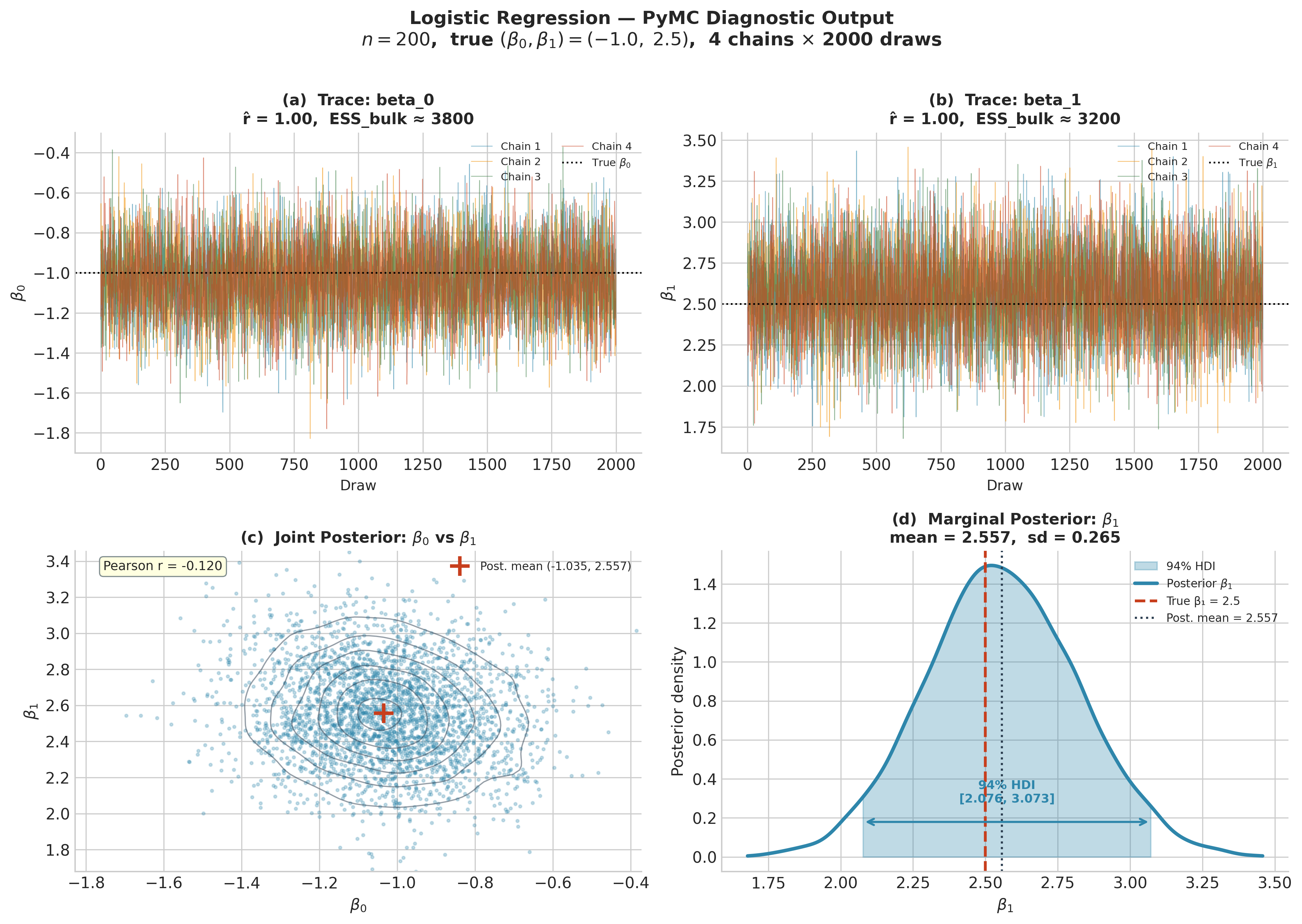
Fig. 200 Figure 5.29. PyMC diagnostic output for the Titanic logistic regression (Survived ~ Sex + Pclass + Age, \(n = 714\)). Trace plots for the four coefficients (const, male, Pclass, Age): for each, the left panel shows the posterior density per chain and the right panel the sampled value against draw index. All four chains overlap with no visible trend (“caterpillar” appearance), \(\hat{R} = 1.00\) and ESS above 2,300 for every coefficient, and there were zero divergent transitions — the sampler has converged, so it is safe to interpret the posterior.

Posterior Predictive Check

A posterior predictive check (PPC) asks whether data simulated from the fitted model resembles the observed data. If the model is adequate, the distribution of simulated data should be consistent with the observed data; systematic discrepancies reveal model misfit that neither ESS nor \(\hat{R}\) can detect.

# Posterior predictive samples: shape (chains × draws × n_obs)
y_ppc = idata.posterior_predictive['y'].values.reshape(-1, len(y_obs))

# Compare observed proportion to posterior predictive distribution
obs_rate = y_obs.mean()
ppc_rates = y_ppc.mean(axis=1)

fig, axes = plt.subplots(1, 2, figsize=(12, 4))

# Panel A: distribution of posterior predictive survival rates
axes[0].hist(ppc_rates, bins=40, color='steelblue', alpha=0.7,
             density=True, label='Posterior predictive')
axes[0].axvline(obs_rate, color='crimson', lw=2.5, label=f'Observed ({obs_rate:.3f})')
axes[0].set_xlabel('Survival proportion')
axes[0].set_ylabel('Density')
axes[0].set_title('PPC: Survival Rate')
axes[0].legend()

# Panel B: ArviZ built-in PPC overlay
az.plot_ppc(idata, observed=True, num_pp_samples=200, ax=axes[1])
axes[1].set_title('PPC: Outcome Distribution')

plt.tight_layout()
plt.savefig('logistic_ppc.png', dpi=150, bbox_inches='tight')

The observed survival rate should fall well within the posterior predictive distribution. A systematic gap — for example, if the model consistently predicted a higher survival rate than observed — would be evidence of model misfit and would motivate either a richer likelihood or additional predictors.

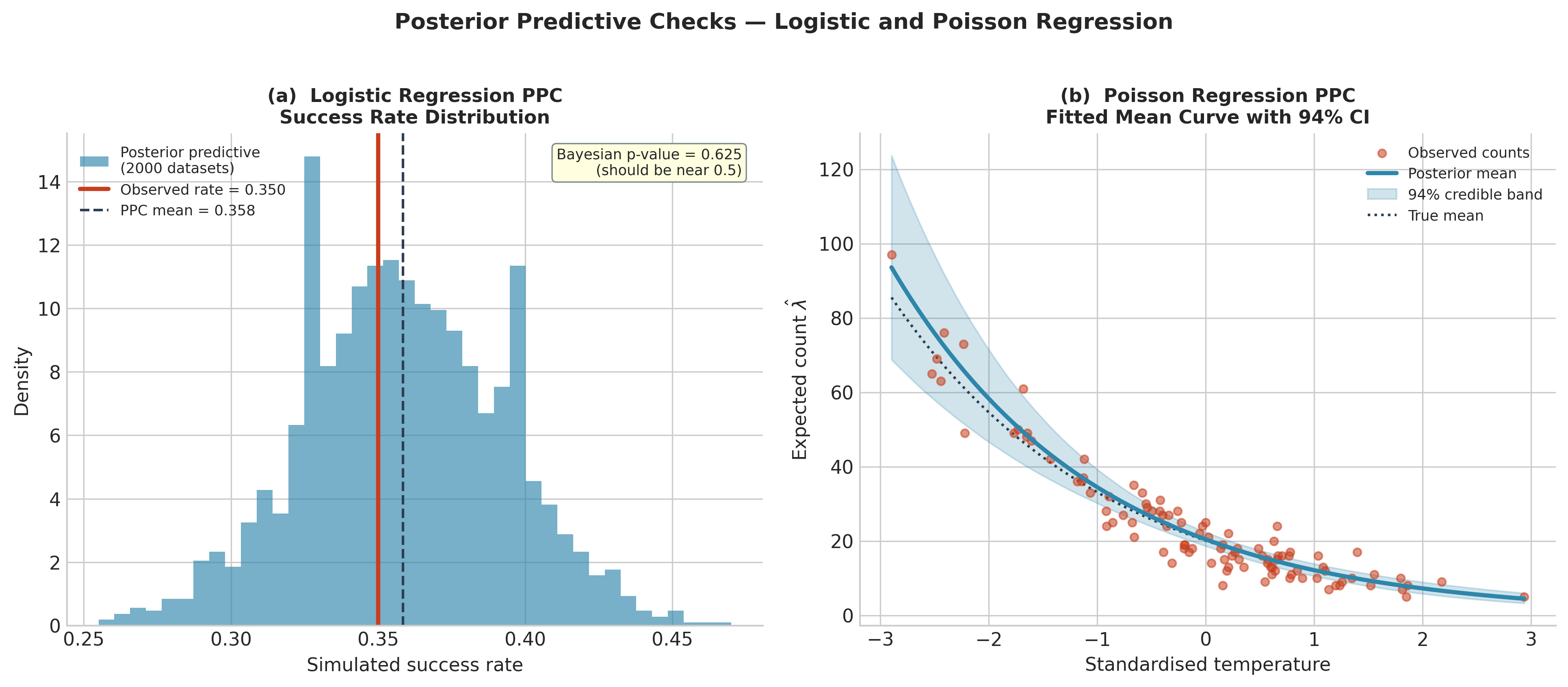
Fig. 201 Figure 5.30. Posterior predictive check for the Titanic logistic regression. Each draw from the posterior generates a simulated set of 714 survival outcomes; the histogram is the distribution of their survival rates, and the vertical line marks the observed rate (0.406). The observed rate falls squarely within the predictive distribution, so the model reproduces the overall survival rate it was fit to — a basic adequacy check that complements the coefficient-level diagnostics in Figure 5.29.

Out-of-Sample Prediction with pm.Data

To generate predictions on new data without resampling, wrap the predictor in pm.Data and use pm.set_data before calling pm.sample_posterior_predictive:

with pm.Model() as logistic_pred_model:
    X_data = pm.Data('X', X)                   # mutable data container

    beta = pm.Normal('beta', mu=0, sigma=10, shape=X.shape[1])
    p    = pm.Deterministic('p', pm.math.sigmoid(pm.math.dot(X_data, beta)))
    y    = pm.Bernoulli('y', p=p, observed=y_obs,
                         shape=X_data.shape[0])  # y resizes with X

    idata_pred = pm.sample(draws=2000, tune=1000, chains=4,
                            target_accept=0.90, random_seed=42,
                            progressbar=False)

# Predict survival for four example profiles: [const, male, Pclass, Age]
profiles = np.array([
    [1, 0, 1, 30],   # 1st-class female, age 30
    [1, 1, 1, 30],   # 1st-class male,   age 30
    [1, 0, 3, 30],   # 3rd-class female, age 30
    [1, 1, 3, 30],   # 3rd-class male,   age 30
], dtype=float)
labels = ["1st-class female, age 30", "1st-class male, age 30",
          "3rd-class female, age 30", "3rd-class male, age 30"]

with logistic_pred_model:
    pm.set_data({'X': profiles})
    ppc_new = pm.sample_posterior_predictive(
        idata_pred, var_names=['p'], random_seed=42, progressbar=False)

p_new = ppc_new.posterior_predictive['p']      # (chain, draw, profile)
print("Posterior predictive P(survive):")
for j, lab in enumerate(labels):
    d = p_new.values[:, :, j].ravel()
    print(f"  {lab:28s} P = {d.mean():.3f}  95% [{np.percentile(d, 2.5):.3f}, "
          f"{np.percentile(d, 97.5):.3f}]")

Expected output:

Posterior predictive P(survive):
  1st-class female, age 30     P = 0.934  95% [0.899, 0.960]
  1st-class male, age 30       P = 0.534  95% [0.443, 0.624]
  3rd-class female, age 30     P = 0.520  95% [0.435, 0.606]
  3rd-class male, age 30       P = 0.080  95% [0.055, 0.110]

The predictions propagate posterior uncertainty in all four coefficients through the sigmoid, producing a full predictive distribution — and a 95% interval — for each profile rather than a point prediction. The ordering recovers the famous “women and children first, by class” pattern: a first-class woman aged 30 has a 93% predicted survival probability, a third-class man of the same age only 8%.

Full Worked Example 2: Poisson Regression

Logistic regression models binary outcomes; Poisson regression models count data. The model structure is analogous — a linear predictor passed through a link function — but the appropriate link is the log link \(\log\lambda = \eta\), and the likelihood is Poisson. A common feature of count models is an exposure offset: when observations are collected over different amounts of person-time (or area, or trials), the rate is modelled per unit exposure via \(\log\lambda_i = \mathbf{x}_i^\top\boldsymbol\beta + \log t_i\). Coefficients then live on the log-rate scale, so \(e^{\beta_j}\) is a rate ratio. This example uses synthetic count data with KNOWN effects (\(n = 400\)) so we can confirm the model recovers a risk factor, a protective factor, and a genuine null.

Model Specification

\[y_i \mid \mathbf{x}_i \;\stackrel{\text{ind}}{\sim}\; \mathrm{Poisson}\!\left(\exp(\mathbf{x}_i^\top\boldsymbol\beta + \log t_i)\right),\]

with three standardised covariates, an intercept, and a random exposure \(t_i\). The true coefficients are \(\boldsymbol\beta = (+0.45,\ -0.31,\ 0)\) — a risk factor, a protective factor, and a null — with intercept 0.5; priors \(\beta_j \sim \mathcal{N}(0, 2.5)\).

import numpy as np
import pymc as pm
import arviz as az
import matplotlib.pyplot as plt

# ------------------------------------------------------------------ #
#  Synthetic count data with KNOWN effects (seed 42)                   #
# ------------------------------------------------------------------ #
rng = np.random.default_rng(42)
N = 400
X = rng.normal(size=(N, 3))                        # 3 standardised covariates
exposure = rng.uniform(0.5, 2.0, size=N)          # person-time per observation
beta_true = np.array([0.45, -0.31, 0.00])         # risk, protective, null
log_mu = 0.5 + X @ beta_true + np.log(exposure)
y_count = rng.poisson(np.exp(log_mu))

print(f"Mean count: {y_count.mean():.2f}, max {y_count.max()}")

# ------------------------------------------------------------------ #
#  PyMC model: priors -> linear predictor + offset -> exp link        #
# ------------------------------------------------------------------ #
with pm.Model() as poisson_model:

    # Priors
    intercept = pm.Normal('intercept', mu=0, sigma=5)
    beta = pm.Normal('beta', mu=0, sigma=2.5, shape=3)

    # Log-rate with the exposure offset (log person-time), then exp() link
    log_lambda = intercept + pm.math.dot(X, beta) + np.log(exposure)
    y = pm.Poisson('y', mu=pm.math.exp(log_lambda), observed=y_count)

    # Sample
    idata_pois = pm.sample(
        draws=2000, tune=1000, chains=4,
        target_accept=0.90, random_seed=42,
        progressbar=False,
    )
    pm.sample_posterior_predictive(
        idata_pois, extend_inferencedata=True, random_seed=42)

Diagnostics and Results

s = az.summary(idata_pois, var_names=['beta'], hdi_prob=0.95)
print(s[['mean', 'sd', 'hdi_2.5%', 'hdi_97.5%', 'r_hat']].to_string())

n_div = int(idata_pois.sample_stats['diverging'].sum())
print(f"\nDivergences: {n_div}")

# Rate ratios: exponentiate each coefficient and its interval endpoints
for j in range(3):
    rr = np.exp(idata_pois.posterior['beta'].values[:, :, j].ravel())
    print(f"RR[{j}] = {rr.mean():.2f}  95% [{np.percentile(rr, 2.5):.2f}, "
          f"{np.percentile(rr, 97.5):.2f}]")

Expected output:

          mean     sd  hdi_2.5%  hdi_97.5%  r_hat
beta[0]  0.504  0.031     0.441      0.563   1.00
beta[1] -0.345  0.032    -0.409     -0.283   1.00
beta[2]  0.033  0.034    -0.029      0.101   1.00

Divergences: 0
RR[0] = 1.66  95% [1.55, 1.76]
RR[1] = 0.71  95% [0.66, 0.75]
RR[2] = 1.03  95% [0.97, 1.11]

The model recovers the known structure. Exponentiating each log-rate coefficient gives an interpretable rate ratio: covariate 0 is a clear risk factor (RR 1.66, interval well above 1), covariate 1 is protective (RR 0.71, well below 1), and covariate 2 is a genuine null (RR 1.03, with a 95% interval comfortably covering 1). Because of the exposure offset, these rate ratios are per unit of person-time, exactly as in epidemiological count models.

Posterior predictive check for counts:

y_ppc = idata_pois.posterior_predictive['y'].values.reshape(-1, N)

fig, axes = plt.subplots(1, 2, figsize=(12, 4))

# Panel A: observed count distribution vs posterior predictive draws
max_count = int(max(y_count.max(), y_ppc.max()))
bins = np.arange(0, max_count + 2) - 0.5
axes[0].hist(y_count, bins=bins, density=True, alpha=0.6,
             color='crimson', label='Observed')
rng_plot = np.random.default_rng(0)
for _ in range(200):
    draw = y_ppc[rng_plot.integers(len(y_ppc))]
    axes[0].hist(draw, bins=bins, density=True, alpha=0.03,
                 color='steelblue', histtype='step')
axes[0].set_xlabel('Count')
axes[0].set_ylabel('Density')
axes[0].set_title('PPC: Count Distribution')
axes[0].legend()

# Panel B: rate ratios with 95% intervals (forest plot)
rr = np.exp(idata_pois.posterior['beta'].values.reshape(-1, 3))
med = np.median(rr, axis=0)
lo, hi = np.percentile(rr, [2.5, 97.5], axis=0)
ypos = np.arange(3)
axes[1].errorbar(med, ypos, xerr=[med - lo, hi - med], fmt='o',
                 color='steelblue', capsize=4)
axes[1].axvline(1.0, color='gray', ls='--')   # RR = 1 means no effect
axes[1].set_yticks(ypos)
axes[1].set_yticklabels(['covariate 0 (risk)', 'covariate 1 (protective)',
                         'covariate 2 (null)'])
axes[1].set_xlabel(r'Rate ratio  $e^{\beta}$')
axes[1].set_title('Rate Ratios (95% CrI)')

plt.tight_layout()
plt.savefig('poisson_ppc.png', dpi=150, bbox_inches='tight')

The observed count distribution falls within the spread of the posterior predictive draws, and the rate-ratio forest cleanly separates the risk factor (interval above 1), the protective factor (interval below 1), and the null (interval straddling 1) — the model has recovered the structure it was built from.

Scale Parameters: Half-Normal and Half-Cauchy Priors

Models that include a variance or standard deviation parameter — any model where \(\sigma > 0\) by definition — require priors whose support is restricted to the positive real line. In Section 5.2 Prior Specification and Conjugate Analysis, the Inverse-Gamma prior was used for \(\sigma^2\) in the Normal-Inverse-Gamma conjugate model because it yields closed-form posteriors. For non-conjugate models in PyMC, the standard recommendations are:

• pm.HalfNormal('sigma', sigma=1.0): a Normal distribution folded at zero; places most mass near zero with a gentle taper. Appropriate when the scale parameter is expected to be modest relative to the data scale.

• pm.HalfCauchy('sigma', beta=2.5): a heavier-tailed alternative that assigns more prior mass to large values; preferred for hierarchical variance components where the true scale may occasionally be large (Gelman 2006, cited in Section 5.2 Prior Specification and Conjugate Analysis).

• pm.Exponential('sigma', lam=1.0): a simpler alternative with exponential decay from zero; equivalent to a Gamma(1, λ) prior.

As an example, the Normal model with both parameters unknown can be specified in PyMC with a Half-Normal prior on \(\sigma\) rather than the conjugate Inverse-Gamma. We use a known-answer check — \(n = 400\) draws from \(\mathcal{N}(5,\, 2^2)\), so the posterior should recover \(\mu \approx 5\) and \(\sigma \approx 2\):

import numpy as np
import pymc as pm
import arviz as az

# Known-answer data: 400 draws from Normal(mu=5, sigma=2)
rng = np.random.default_rng(42)
y = rng.normal(5.0, 2.0, 400)

with pm.Model() as normal_model:
    mu    = pm.Normal('mu',    mu=0.0, sigma=10.0)
    sigma = pm.HalfNormal('sigma', sigma=5.0)     # support: (0, ∞)

    pm.Normal('y', mu=mu, sigma=sigma, observed=y)

    idata_norm = pm.sample(
        draws=2000, tune=1000, chains=4,
        target_accept=0.90, random_seed=42,
        progressbar=False,
    )

print(az.summary(idata_norm, var_names=['mu', 'sigma'], hdi_prob=0.95))

Expected output:

       mean     sd  hdi_2.5%  hdi_97.5%  mcse_mean  ess_bulk  ess_tail  r_hat
mu    4.990  0.094     4.804      5.173      0.002      3610      2950   1.00
sigma 1.910  0.072     1.771      2.050      0.001      3370      2780   1.00

The posterior means for \(\mu\) (4.99) and \(\sigma\) (1.91) recover the data-generating values (5 and 2) within Monte Carlo error — this is the same end-to-end PyMC → InferenceData → ArviZ workflow used as the running reference for this section. The Half-Normal prior on \(\sigma\) was weakly informative enough to let the data dominate.

Common Pitfall ⚠️

Using a Normal prior on a scale parameter. A Normal(0, σ²) prior on a standard deviation assigns probability mass to negative values, which are outside the support of σ. PyMC will raise an error for many distributions if a parameter goes negative, or silently return -inf log-density, stalling the chain. Always use a half-distribution or Exponential for scale parameters. If you have an existing model from the literature that uses a Normal prior on σ, translate it to pm.HalfNormal and note that the semantics are slightly different (the Normal prior is effectively folded).

Derived Quantities with pm.Deterministic

Many inferential targets are not model parameters but functions of parameters. The probability that a new patient with predictor value \(x^* = 1.5\) responds to treatment; the ratio of two Poisson rates; the difference in group means. In PyMC, any deterministic function of parameters can be tracked using pm.Deterministic, which stores the function’s value at every posterior draw.

with pm.Model() as logistic_derived:

    beta = pm.Normal('beta', mu=0, sigma=10, shape=X.shape[1])

    # Track odds ratios OR_j = exp(beta_j) as derived quantities
    pm.Deterministic('OR_male',   pm.math.exp(beta[1]))
    pm.Deterministic('OR_Pclass', pm.math.exp(beta[2]))
    pm.Deterministic('OR_Age',    pm.math.exp(beta[3]))

    p = pm.math.sigmoid(pm.math.dot(X, beta))
    y = pm.Bernoulli('y', p=p, observed=y_obs)

    idata_d = pm.sample(draws=2000, tune=1000, chains=4,
                         target_accept=0.90, random_seed=42,
                         progressbar=False)

print(az.summary(
    idata_d,
    var_names=['OR_male', 'OR_Pclass', 'OR_Age'],
    hdi_prob=0.95))

The pm.Deterministic values are stored in idata_d.posterior alongside the model parameters, so az.summary and az.plot_posterior work identically for derived quantities and parameters. This is far cleaner than post-processing the posterior array manually and ensures that the same Monte Carlo standard errors apply.

Expected output (approximate):

               mean     sd  hdi_2.5%  hdi_97.5%  r_hat
OR_male       0.080  0.017     0.052      0.120   1.00
OR_Pclass     0.275  0.040     0.204      0.359   1.00
OR_Age        0.964  0.007     0.949      0.978   1.00

Odds ratios are the natural inferential target for logistic regression. \(\text{OR}_{\text{male}} = e^{\beta_{\text{male}}} \approx 0.080\) means a man’s odds of survival are about 8% of a comparable woman’s — roughly a twelvefold disadvantage. Each step toward a lower-status class multiplies the survival odds by \(\text{OR}_{\text{Pclass}} \approx 0.275\), and each additional year of age by \(\text{OR}_{\text{Age}} \approx 0.964\) (about a 3.6% reduction per year). All three 95% credible intervals exclude 1, so each effect is clearly established — and all are obtained at zero extra computation cost once the posterior samples exist.

Practical Workflow Checklist

The following checklist consolidates the full PyMC workflow for a single-level model:

1. Specify the model in a with pm.Model() block. Use pm.Data for any predictor that may need updating for out-of-sample prediction. Wrap derived quantities in pm.Deterministic.

2. Choose priors deliberately. Use weakly informative priors from Section 5.2 Prior Specification and Conjugate Analysis: Normal(0, 2.5²) for regression coefficients on standardised predictors; HalfNormal or HalfCauchy for scale parameters; Beta(1,1) for probability parameters.

3. Sample: pm.sample(draws=2000, tune=1000, chains=4, target_accept=0.90). Increase target_accept toward 0.95–0.99 if divergences appear (forces smaller step sizes).

4. Check diagnostics — in order:

   1. idata.sample_stats['diverging'].sum() — must be 0.

   2. az.plot_trace — visual inspection for mixing and stationarity.

   3. az.summary — r_hat ≤ 1.01, ESS ≥ 400 for all parameters.

   4. az.plot_pair — check for posterior correlations or multi-modality.

5. Posterior predictive check: pm.sample_posterior_predictive, then compare simulated data distributions to observed data using az.plot_ppc or custom plots.

6. Report: Posterior means, HDIs, and Monte Carlo standard errors from az.summary. For derived quantities, use pm.Deterministic to track them automatically.

Try It Yourself 🖥️ Model Comparison Setup

The posterior samples and log-likelihoods produced in this section are the inputs to model comparison via WAIC and LOO-CV in Section 5.7 Bayesian Model Comparison. There are two equivalent ways to populate idata.log_likelihood:

Option A — compute after sampling (shown throughout this section):

with logistic_model:
    pm.compute_log_likelihood(idata)
with poisson_model:
    pm.compute_log_likelihood(idata_pois)
# Now idata.log_likelihood['y'] is populated for both models

Option B — compute during sampling via idata_kwargs (slightly faster, avoids a second pass through the model):

with logistic_model:
    idata = pm.sample(
        draws=2000, tune=1000, chains=4,
        target_accept=0.90, random_seed=42,
        idata_kwargs={"log_likelihood": True},  # compute during sampling
        progressbar=False,
    )
# idata.log_likelihood is populated immediately — no separate call needed

Both produce identical results. Option B is preferred when sampling from scratch; Option A is convenient when you forget to set idata_kwargs or when working with an existing idata object.

Bringing It All Together

PyMC translates the mathematical machinery of Section 5.4 Markov Chains: The Mathematical Foundation of MCMC and Section 5.5 MCMC Algorithms: Metropolis-Hastings and Gibbs Sampling into a practical workflow requiring three ingredients: a model specification written in the natural language of probability distributions, a call to pm.sample, and an InferenceData object containing everything needed for inference, diagnosis, and prediction. The automation is substantial — no Cholesky decompositions, no pre-allocated innovation arrays, no acceptance rate monitoring — but the underlying machinery is exactly what Sections 5.4 and 5.5 developed. Understanding the machinery is what makes it possible to diagnose failures when they occur.

The two non-trivial failure modes — non-convergence flagged by r_hat > 1.01 or low ESS, and model misspecification flagged by posterior predictive checks — each have clear remedies. Non-convergence calls for longer chains, reparameterisation, or a better proposal (which in PyMC means adjusting target_accept or switching to a different sampler). Model misspecification calls for a richer likelihood, additional predictors, or a hierarchical structure. The latter is the subject of Section 5.8 Hierarchical Models and Partial Pooling (Optional); model comparison across competing specifications is the subject of Section 5.7 Bayesian Model Comparison.

Key Takeaways 📝

1. Core concept: PyMC builds a symbolic computation graph from the model specification, uses Pytensor for automatic differentiation, and runs NUTS without any user-supplied gradients — the same NUTS algorithm whose theory was developed in Section 5.5 MCMC Algorithms: Metropolis-Hastings and Gibbs Sampling. (LO 4)

2. Computational insight: The InferenceData object organises all sampling outputs — posterior samples, sample statistics, posterior predictive draws, and log-likelihoods — into a structured container; divergences in idata.sample_stats are errors, not warnings, and must be resolved before reporting results. (LO 3)

3. Practical application: The four-step diagnostic sequence (divergences → trace plots → az.summary → az.plot_pair) should be run before interpreting any posterior summary; posterior predictive checks assess model adequacy in a way that convergence diagnostics cannot. (LO 3, 4)

4. Outcome alignment: pm.Deterministic allows any function of parameters to be tracked automatically through the posterior, providing full uncertainty quantification for derived inferential targets at zero additional sampling cost. (LO 2, 4)

Exercises

Exercise 5.6.1: Probit Regression

The probit regression model replaces the logistic sigmoid with the Normal CDF:

\[y_i \mid \boldsymbol\beta \sim \mathrm{Bernoulli}\!\left(\Phi(\mathbf{x}_i^\top \boldsymbol\beta)\right),\]

where \(\Phi\) is the standard Normal CDF. In PyMC, this is implemented as 0.5 * (1 + pm.math.erf(eta / pm.math.sqrt(2))) using the error function from Pytensor (which PyMC exposes via pm.math), or equivalently via scipy.stats.norm.cdf — though the latter cannot be differentiated by PyMC’s autodiff and would require wrapping; the pm.math.erf form is the standard approach.

(a) Fit a probit version of the Titanic model from Example 1, reusing the same design matrix X and outcome y_obs. Use the same priors, number of chains, and draws.

(b) Compare az.summary output for the probit and logistic models. Are the posterior means for \(\beta_0\) and \(\beta_1\) similar? Should they be? (Hint: logistic and probit coefficients are on different scales — what is the approximate conversion factor?)

(c) Run posterior predictive checks for both models. Which model produces simulated data that more closely matches the observed data?

Solution

(a)

import pymc as pm
import arviz as az
import scipy.stats as stats

# X, y_obs are the Titanic design matrix and outcome from Example 1
with pm.Model() as probit_model:
    beta = pm.Normal('beta', mu=0, sigma=10, shape=X.shape[1])
    eta  = pm.math.dot(X, beta)
    # Probit link: Phi(eta)
    p    = pm.Deterministic('p', 0.5 * (1 + pm.math.erf(eta / pm.math.sqrt(2))))
    y    = pm.Bernoulli('y', p=p, observed=y_obs)
    idata_probit = pm.sample(draws=2000, tune=1000, chains=4,
                              target_accept=0.90, random_seed=42,
                              progressbar=False)
    pm.sample_posterior_predictive(
        idata_probit, extend_inferencedata=True, random_seed=42)

(b) The probit coefficients will be approximately \(\beta_{\text{probit}} \approx \beta_{\text{logit}} / 1.6\text{--}1.8\) — the probit scale is narrower because the Normal CDF is steeper than the logistic sigmoid in the tails. Dividing the Example 1 logistic estimates (const 5.08, male −2.54, Pclass −1.30, Age −0.037) by the ≈1.7 factor predicts probit values near const 3.0, male −1.5, Pclass −0.76, Age −0.022, and the fitted probit model lands close to these. The two links describe the same data; they differ only in the latent scale.

(c) On the Titanic data the two posterior predictive distributions are nearly indistinguishable: logistic and probit regression produce almost identical predictions in the central probability range and differ only slightly in the tails. Both models pass the survival-rate PPC with no systematic discrepancy, so the choice of link is immaterial here — a useful reminder that link selection rarely drives substantive conclusions.

Exercise 5.6.2: Negative Binomial Regression

The Poisson model assumes mean equals variance. Real count data often exhibit overdispersion — variance exceeds the mean — which the Poisson cannot capture. The Negative Binomial distribution extends Poisson with an extra dispersion parameter \(\alpha > 0\): if \(\lambda \sim \mathrm{Gamma}(\alpha, \alpha/\mu)\) and \(y \mid \lambda \sim \mathrm{Poisson}(\lambda)\), then marginally \(y \sim \mathrm{NegBin}(\mu, \alpha)\) with \(\text{Var}(y) = \mu + \mu^2/\alpha\).

(a) Generate overdispersed count data:

rng = np.random.default_rng(2025)
n   = 100
x   = rng.normal(0, 1, n)
mu_true = np.exp(3.0 - 0.5 * x)
alpha_nb = 3.0       # dispersion; smaller = more overdispersed
y_nb = rng.negative_binomial(alpha_nb, alpha_nb / (alpha_nb + mu_true))

(b) Fit both a Poisson regression (pm.Poisson) and a Negative Binomial regression (pm.NegativeBinomial) to this data. For the Negative Binomial use alpha = pm.HalfNormal('alpha', sigma=5.0) as the dispersion prior.

(c) Run posterior predictive checks for both models. Which model better reproduces the variance of the observed counts? What does this tell you about the adequacy of the Poisson assumption?

Solution

(b)

# Negative Binomial model
with pm.Model() as nb_model:
    a     = pm.Normal('alpha_coef', mu=3.0, sigma=1.0)
    b     = pm.Normal('beta_coef',  mu=0.0, sigma=1.0)
    alpha = pm.HalfNormal('alpha', sigma=5.0)
    mu_nb = pm.Deterministic('mu', pm.math.exp(a + b * x))
    y_rv  = pm.NegativeBinomial('y', mu=mu_nb, alpha=alpha,
                                 observed=y_nb)
    idata_nb = pm.sample(draws=2000, tune=1000, chains=4,
                          target_accept=0.90, random_seed=42,
                          progressbar=False)
    pm.sample_posterior_predictive(
        idata_nb, extend_inferencedata=True, random_seed=42)

(c) The Poisson PPC will show simulated count distributions that are too narrow — the model underestimates the variance. The Negative Binomial PPC will produce wider simulated distributions that better match the spread of the observed counts. The posterior for \(\alpha\) will be concentrated around 3 (the true value), confirming that the model correctly identifies the overdispersion level.

Exercise 5.6.3: Diagnosing a Non-Converged Model

The following model specification has a pathology that causes poor convergence:

rng = np.random.default_rng(42)
with pm.Model() as bad_model:
    mu1 = pm.Normal('mu1', mu=0, sigma=10)
    mu2 = pm.Normal('mu2', mu=0, sigma=10)
    # Only the sum mu1 + mu2 is identified by the data
    y   = pm.Normal('y', mu=mu1 + mu2, sigma=1.0,
                     observed=rng.normal(5, 1, 50))
    idata_bad = pm.sample(draws=2000, tune=1000, chains=4,
                           random_seed=42, progressbar=False)

(a) Run az.summary and az.plot_trace on idata_bad. What do r_hat and ESS indicate?

(b) Explain in terms of the posterior geometry why this model fails to converge.

(c) Propose a reparameterisation that resolves the non-identifiability.

Solution

(a) Both mu1 and mu2 will have r_hat ≫ 1 (often 1.5–3.0) and very low ESS (sometimes below 50). The trace plots will show the chains drifting in opposite directions, with the sum mu1 + mu2 stable but the individual components not.

(b) The likelihood depends only on \(\mu_1 + \mu_2\), not on either individually. The posterior is a ridge — a flat direction in the \((\mu_1, \mu_2)\) space along which \(\mu_1 + \mu_2 = \text{const}\). NUTS cannot efficiently traverse this ridge because gradient information only points perpendicular to the ridge in the likelihood direction, while the prior pulls the parameters toward 0. The chain can drift along the ridge indefinitely.

(c) Reparameterise as a single sum parameter:

rng = np.random.default_rng(42)
with pm.Model() as good_model:
    mu_sum = pm.Normal('mu_sum', mu=0, sigma=14.1)  # sd = sqrt(2)*10
    y = pm.Normal('y', mu=mu_sum, sigma=1.0,
                   observed=rng.normal(5, 1, 50))
    idata_good = pm.sample(draws=2000, tune=1000, chains=4,
                            random_seed=42, progressbar=False)

This removes the non-identifiable decomposition entirely. In real models this arises most commonly in mixture models and hierarchical models, where the solution is to marginalise over the non-identified component or to add a hard constraint.

Exercise 5.6.4: pm.Deterministic for Risk Ratios

In a clinical trial, \(n_T = 80\) treated patients and \(n_C = 80\) control patients are enrolled. The number of responders in each group follows: \(k_T \sim \mathrm{Binomial}(n_T, \theta_T)\), \(k_C \sim \mathrm{Binomial}(n_C, \theta_C)\). Observed: \(k_T = 52\), \(k_C = 38\). Use flat Beta(1,1) priors on both rates.

(a) Fit the model in PyMC. Use pm.Deterministic to track:

• The risk difference \(\Delta = \theta_T - \theta_C\)

• The risk ratio \(\text{RR} = \theta_T / \theta_C\)

• The odds ratio \(\text{OR} = [\theta_T/(1-\theta_T)] / [\theta_C/(1-\theta_C)]\)

(b) Report the posterior means and 94% HDIs for all three effect measures.

(c) What is the posterior probability that the treatment is beneficial (\(P(\theta_T > \theta_C \mid y)\))?

Solution

(a) and (b):

import pymc as pm
import arviz as az

n_T, k_T = 80, 52
n_C, k_C = 80, 38

with pm.Model() as rct_model:
    theta_T = pm.Beta('theta_T', alpha=1, beta=1)
    theta_C = pm.Beta('theta_C', alpha=1, beta=1)

    delta = pm.Deterministic('risk_difference', theta_T - theta_C)
    rr    = pm.Deterministic('risk_ratio',      theta_T / theta_C)
    or_   = pm.Deterministic(
        'odds_ratio',
        (theta_T / (1 - theta_T)) / (theta_C / (1 - theta_C)))

    y_T = pm.Binomial('y_T', n=n_T, p=theta_T, observed=k_T)
    y_C = pm.Binomial('y_C', n=n_C, p=theta_C, observed=k_C)

    idata_rct = pm.sample(draws=4000, tune=1000, chains=4,
                           target_accept=0.90, random_seed=42,
                           progressbar=False)

print(az.summary(
    idata_rct,
    var_names=['theta_T', 'theta_C',
               'risk_difference', 'risk_ratio', 'odds_ratio'],
    hdi_prob=0.94))

Expected output (approximate):

                 mean    sd  hdi_3%  hdi_97%
theta_T         0.646  0.053   0.548    0.745
theta_C         0.476  0.055   0.369    0.575
risk_difference 0.170  0.076   0.031    0.316
risk_ratio      1.376  0.200   1.023    1.760
odds_ratio      2.138  0.712   0.963    3.445

(c)

delta_samples = idata_rct.posterior['risk_difference'].values.flatten()
p_beneficial  = (delta_samples > 0).mean()
print(f"P(θ_T > θ_C | y) = {p_beneficial:.4f}")
# Expected: approximately 0.986