Section 3.4 Linear Models
Linear regression is one of the central tools in statistical modeling. Developed in the early 19th century in connection with astronomical and geodetic problems, least squares is often associated with Legendre and Gauss, and it provided a systematic way to estimate relationships from noisy measurements. Today, linear regression remains a default starting point across the sciences and a core building block for many ideas in modern machine learning. The goal is not simply to run a routine, but to understand the model, the assumptions it encodes, and what its estimates and diagnostics do and do not justify.
This section develops linear regression from first principles. We begin with the matrix calculus needed to derive estimators—building up the rules for differentiating vectors, matrices, and quadratic forms. We then derive the ordinary least squares (OLS) estimator via two complementary approaches: the calculus approach (minimizing sum of squared errors) and the geometric approach (projection onto the column space). These perspectives illuminate different aspects of the same solution.
With the estimator in hand, we prove the Gauss-Markov theorem—that OLS is the Best Linear Unbiased Estimator (BLUE) under specific conditions. We examine each condition carefully, understanding what happens when it fails. We then develop the distributional theory under normality, enabling t-tests, F-tests, and confidence intervals. Finally, we address diagnostics and remedies for when assumptions don’t hold.
Road Map 🧭
Develop: Matrix calculus rules for differentiating vectors, quadratic forms, and matrix products
Derive: OLS estimator via calculus (normal equations) and geometry (projection)
Prove: Gauss-Markov theorem establishing OLS as BLUE under classical assumptions
Apply: Distributional results for inference: t-tests, F-tests, confidence intervals
Evaluate: Diagnostics for assumption violations and remedial measures
Matrix Calculus Foundations
Before deriving the least squares estimator, we need tools for differentiating expressions involving vectors and matrices. This section builds up the necessary calculus systematically, starting from scalar derivatives and extending to the multivariate case. (A condensed reference for these rules — including the gradient identities for linear and quadratic forms — appears in Appendix B.)
Why Matrix Calculus?
In scalar calculus, finding the minimum of \(f(x) = (y - x)^2\) is straightforward: take the derivative, set it to zero, solve for \(x\). With \(n\) observations and \(p\) parameters, our objective becomes:
Minimizing this requires differentiating with respect to a vector \(\boldsymbol{\beta}\). Matrix calculus provides the systematic framework for such operations.
Notation Conventions
We adopt the following conventions throughout:
Vectors are column vectors, denoted by bold lowercase: \(\mathbf{x}, \mathbf{y}, \boldsymbol{\beta}\)
Matrices are denoted by bold uppercase: \(\mathbf{X}, \mathbf{A}, \boldsymbol{\Sigma}\)
Scalars are italic lowercase: \(a, b, \sigma^2\)
Transpose: \(\mathbf{x}^\top\) (row vector), \(\mathbf{A}^\top\)
Dimensions: \(\mathbf{y} \in \mathbb{R}^n\), \(\boldsymbol{\beta} \in \mathbb{R}^p\), \(\mathbf{X} \in \mathbb{R}^{n \times p}\)
The gradient of a scalar function \(f: \mathbb{R}^p \to \mathbb{R}\) with respect to vector \(\boldsymbol{\beta}\) is:
This is a column vector of the same dimension as \(\boldsymbol{\beta}\).
Scalar-by-Vector Derivatives: Building the Rules
We develop the key differentiation rules step by step, starting from component-wise analysis.
Rule 1: Linear function \(f(\boldsymbol{\beta}) = \mathbf{a}^\top \boldsymbol{\beta}\) where \(\mathbf{a} \in \mathbb{R}^p\) is constant.
Component form:
Taking the partial derivative with respect to \(\beta_k\):
Assembling all partials into a vector:
By symmetry of the dot product, \(\mathbf{a}^\top \boldsymbol{\beta} = \boldsymbol{\beta}^\top \mathbf{a}\), so:
Rule 2: Quadratic form \(f(\boldsymbol{\beta}) = \boldsymbol{\beta}^\top \mathbf{A} \boldsymbol{\beta}\) where \(\mathbf{A} \in \mathbb{R}^{p \times p}\) is constant.
Component form:
Taking the partial derivative with respect to \(\beta_k\) requires identifying all terms containing \(\beta_k\):
Terms where \(i = k\) (varying \(j\)): \(\sum_{j=1}^p \beta_k A_{kj} \beta_j\)
Terms where \(j = k\) (varying \(i\)): \(\sum_{i=1}^p \beta_i A_{ik} \beta_k\)
For the first group:
For the second group:
Combining:
Assembling into vector form:
Special case: If \(\mathbf{A}\) is symmetric (\(\mathbf{A} = \mathbf{A}^\top\)):
This is the result we’ll use most often, since \(\mathbf{X}^\top\mathbf{X}\) is always symmetric.
Rule 3: Matrix-vector product \(f(\boldsymbol{\beta}) = \mathbf{A}\boldsymbol{\beta}\) where the result is a vector, not a scalar.
Here \(f: \mathbb{R}^p \to \mathbb{R}^n\), so the derivative is a matrix called the Jacobian:
The \((i, j)\) element is \(\frac{\partial [\mathbf{A}\boldsymbol{\beta}]_i}{\partial \beta_j} = A_{ij}\).
Summary of Key Rules
Expression \(f(\boldsymbol{\beta})\) |
Gradient \(\nabla_{\boldsymbol{\beta}} f\) |
Condition |
|---|---|---|
\(\mathbf{a}^\top \boldsymbol{\beta}\) or \(\boldsymbol{\beta}^\top \mathbf{a}\) |
\(\mathbf{a}\) |
\(\mathbf{a}\) constant |
\(\boldsymbol{\beta}^\top \mathbf{A} \boldsymbol{\beta}\) |
\((\mathbf{A} + \mathbf{A}^\top)\boldsymbol{\beta}\) |
\(\mathbf{A}\) constant |
\(\boldsymbol{\beta}^\top \mathbf{A} \boldsymbol{\beta}\) |
\(2\mathbf{A}\boldsymbol{\beta}\) |
\(\mathbf{A}\) symmetric |
\(\|\mathbf{y} - \mathbf{X}\boldsymbol{\beta}\|^2\) |
\(-2\mathbf{X}^\top(\mathbf{y} - \mathbf{X}\boldsymbol{\beta})\) |
See derivation below |
The Chain Rule for Vectors
For composite functions, we need the chain rule. If \(f: \mathbb{R}^n \to \mathbb{R}\) and \(\mathbf{g}: \mathbb{R}^p \to \mathbb{R}^n\), then for \(h(\boldsymbol{\beta}) = f(\mathbf{g}(\boldsymbol{\beta}))\):
This is the matrix form of the familiar chain rule: derivative of outer function times derivative of inner function.
The Linear Model
With matrix calculus tools in hand, we now formalize the linear regression model.
Model Specification
We observe \(n\) data points \((y_i, \mathbf{x}_i)\) where \(y_i \in \mathbb{R}\) is the response (dependent variable) and \(\mathbf{x}_i \in \mathbb{R}^p\) is the vector of predictors (independent variables, features, covariates).
The linear model posits:
where:
\(\beta_0, \beta_1, \ldots, \beta_{p-1}\) are unknown parameters (coefficients)
\(\varepsilon_i\) is the error term (disturbance, noise)
Matrix notation: Define the design matrix \(\mathbf{X}\) and response vector \(\mathbf{y}\):
The first column of \(\mathbf{X}\) is all ones (for the intercept). The parameter vector is \(\boldsymbol{\beta} = (\beta_0, \beta_1, \ldots, \beta_{p-1})^\top \in \mathbb{R}^p\).
Notation Note
This text indexes coefficients from \(\beta_0\) to \(\beta_{p-1}\), with the intercept as \(\beta_0\) and \(p\) total parameters. Some references instead index from \(\beta_1\) to \(\beta_p\), or write the model with \(p+1\) coefficients explicitly. The two conventions are equivalent; we use \(p\) to keep the dimension of \(\boldsymbol{\beta}\) and the column count of \(\mathbf{X}\) the same symbol throughout.
The model in matrix form:
where \(\boldsymbol{\varepsilon} = (\varepsilon_1, \ldots, \varepsilon_n)^\top\).
What “Linear” Means
The model (53) is linear in the parameters \(\boldsymbol{\beta}\), not necessarily in the predictors. All of the following are linear models:
Each involves \(y\) as a linear combination of \(\boldsymbol{\beta}\). The following is not a linear model:
Here \(y\) is nonlinear in \(\beta_1\).
Interpreting Coefficients
Before diving into estimation, let’s clarify what the coefficients mean:
Partial slopes: In multiple regression, \(\beta_j\) represents the expected change in \(y\) for a one-unit increase in \(x_j\), holding all other predictors fixed. This “ceteris paribus” interpretation is fundamental.
Correlation vs. causation: The OLS coefficient \(\hat{\beta}_j\) measures the association between \(x_j\) and \(y\), not necessarily a causal effect. To interpret \(\beta_j\) causally, we need:
No omitted confounders (variables that affect both \(x_j\) and \(y\))
No reverse causation (\(y\) doesn’t cause \(x_j\))
No measurement error in predictors
These are strong assumptions rarely satisfied in observational data. Experimental design (randomization) or quasi-experimental methods (instrumental variables, regression discontinuity) are needed for causal claims.
Effect of correlation among predictors: When predictors are correlated, “holding other predictors fixed” may describe a scenario rarely observed in the data. The coefficient \(\beta_j\) still has a well-defined mathematical interpretation, but its practical meaning becomes murky. High multicollinearity inflates standard errors, making individual coefficients imprecise even when the overall model predicts well.
Assumptions: The Classical Linear Model
The linear model (52) comes with assumptions about the errors \(\boldsymbol{\varepsilon}\). We distinguish two levels:
Gauss-Markov Assumptions (for OLS to be BLUE):
Assumption (GM1): Linearity
The true relationship is \(\mathbf{y} = \mathbf{X}\boldsymbol{\beta} + \boldsymbol{\varepsilon}\) for some \(\boldsymbol{\beta} \in \mathbb{R}^p\).
Assumption (GM2): Full Rank
The design matrix \(\mathbf{X}\) has full column rank: \(\text{rank}(\mathbf{X}) = p\).
Equivalently, \(\mathbf{X}^\top\mathbf{X}\) is invertible. This requires \(n \geq p\) and no exact multicollinearity among predictors.
Assumption (GM3): Strict Exogeneity
The errors have zero conditional mean given \(\mathbf{X}\):
This implies \(\mathbb{E}[\varepsilon_i | \mathbf{X}] = 0\) for each \(i\). Predictors are uncorrelated with errors.
Assumption (GM4): Homoskedastic and Uncorrelated Errors
The errors are homoskedastic and uncorrelated:
This means:
Homoskedasticity: \(\text{Var}(\varepsilon_i | \mathbf{X}) = \sigma^2\) for all \(i\) (constant variance)
No autocorrelation: \(\text{Cov}(\varepsilon_i, \varepsilon_j | \mathbf{X}) = 0\) for \(i \neq j\)
(This condition is sometimes called “spherical errors” because the error covariance is a scaled identity matrix.)
Normality Assumption (for exact inference):
Assumption (GM5): Normal Errors
The errors follow a multivariate normal distribution:
This implies GM3 and GM4, plus enables exact t-tests and F-tests. Note that this is specifically the spherical normal model \(\mathcal{N}(\mathbf{0}, \sigma^2 \mathbf{I})\), not merely “some normal covariance”—normality alone does not guarantee homoskedasticity or independence.
The assumptions form a hierarchy:
GM1-GM2: OLS is well-defined (unique solution exists)
GM1-GM4: OLS is BLUE (Gauss-Markov theorem applies)
GM1-GM5: Exact finite-sample inference (t, F distributions)
Ordinary Least Squares: The Calculus Approach
The Ordinary Least Squares (OLS) estimator minimizes the sum of squared residuals:
We find \(\hat{\boldsymbol{\beta}}\) that minimizes RSS by taking the derivative and setting it to zero.
Expanding the Objective Function
First, expand the quadratic form:
Since \(\mathbf{y}^\top\mathbf{X}\boldsymbol{\beta}\) is a scalar, it equals its transpose \(\boldsymbol{\beta}^\top\mathbf{X}^\top\mathbf{y}\):
Taking the Derivative
Using our matrix calculus rules:
\(\nabla_{\boldsymbol{\beta}}(\mathbf{y}^\top\mathbf{y}) = \mathbf{0}\) (constant in \(\boldsymbol{\beta}\))
\(\nabla_{\boldsymbol{\beta}}(2\boldsymbol{\beta}^\top\mathbf{X}^\top\mathbf{y}) = 2\mathbf{X}^\top\mathbf{y}\) (Rule 1: linear form with \(\mathbf{a} = \mathbf{X}^\top\mathbf{y}\))
\(\nabla_{\boldsymbol{\beta}}(\boldsymbol{\beta}^\top\mathbf{X}^\top\mathbf{X}\boldsymbol{\beta}) = 2\mathbf{X}^\top\mathbf{X}\boldsymbol{\beta}\) (Rule 2: quadratic form with symmetric \(\mathbf{A} = \mathbf{X}^\top\mathbf{X}\))
Combining:
The Normal Equations
Setting the gradient to zero:
Rearranging:
These are the normal equations. The name comes from the fact that the residual vector \(\mathbf{y} - \mathbf{X}\hat{\boldsymbol{\beta}}\) is normal (perpendicular) to the column space of \(\mathbf{X}\)—a fact we’ll prove geometrically.
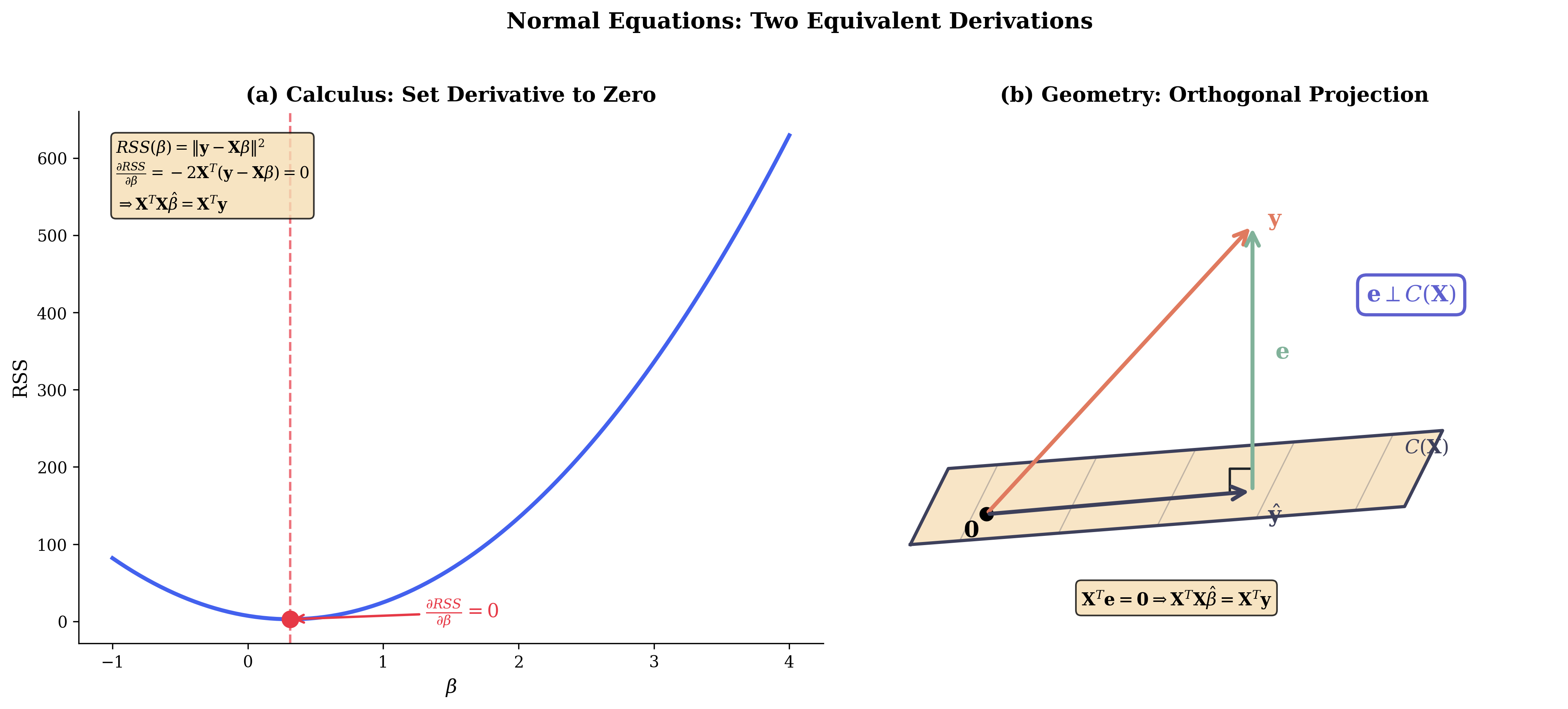
Fig. 81 Figure 3.4.2: The normal equations derived two ways. (a) The calculus approach: minimize RSS by setting the gradient to zero. (b) The geometric approach: the residual \(\mathbf{e}\) must be perpendicular to \(C(\mathbf{X})\), leading to \(\mathbf{X}^\top\mathbf{e} = \mathbf{0}\).
Solving for the OLS Estimator
Under assumption GM2 (\(\text{rank}(\mathbf{X}) = p\)), the matrix \(\mathbf{X}^\top\mathbf{X}\) is invertible. Multiplying both sides by \((\mathbf{X}^\top\mathbf{X})^{-1}\):
This is the OLS estimator—the central result of regression analysis.
Verifying the Minimum
We found a critical point. To confirm it’s a minimum (not maximum or saddle), examine the second derivative (Hessian):
Since \(\mathbf{X}^\top\mathbf{X}\) is positive semi-definite (for any \(\mathbf{v}\), \(\mathbf{v}^\top\mathbf{X}^\top\mathbf{X}\mathbf{v} = \|\mathbf{X}\mathbf{v}\|^2 \geq 0\)), and positive definite when \(\mathbf{X}\) has full column rank, the Hessian is positive definite. Therefore, the critical point is indeed a global minimum.
Example 💡 Simple Linear Regression by Hand
Consider simple regression \(y = \beta_0 + \beta_1 x + \varepsilon\) with \(n = 4\) observations:
Step 1: Compute \(\mathbf{X}^\top\mathbf{X}\):
Step 2: Compute \(\mathbf{X}^\top\mathbf{y}\):
Step 3: Compute \((\mathbf{X}^\top\mathbf{X})^{-1}\):
Step 4: Compute \(\hat{\boldsymbol{\beta}}\):
The fitted line is \(\hat{y} = 0.15 + 1.94x\).
import numpy as np

# Data
X = np.array([[1, 1], [1, 2], [1, 3], [1, 4]])
y = np.array([2.1, 3.9, 6.2, 7.8])

# OLS via normal equations
XtX = X.T @ X
Xty = X.T @ y
beta_hat = np.linalg.solve(XtX, Xty)  # More stable than explicit inverse

print("X'X =")
print(XtX)
print(f"\nX'y = {Xty}")
print(f"\nOLS estimates: β̂₀ = {beta_hat[0]:.4f}, β̂₁ = {beta_hat[1]:.4f}")

# Verify with fitted values
y_hat = X @ beta_hat
residuals = y - y_hat
RSS = np.sum(residuals**2)
print(f"\nFitted values: {y_hat}")
print(f"Residuals: {residuals}")
print(f"RSS = {RSS:.4f}")
X'X =
[[ 4 10]
 [10 30]]

X'y = [20.  59.7]

OLS estimates: β̂₀ = 0.1500, β̂₁ = 1.9400

Fitted values: [2.09 4.03 5.97 7.91]
Residuals: [ 0.01 -0.13  0.23 -0.11]
RSS = 0.0820
Ordinary Least Squares: The Geometric Approach
The calculus approach found the OLS estimator by optimization. The geometric approach reveals why the normal equations work and provides deeper insight into what OLS does.
Column Space and Projection
Consider the design matrix \(\mathbf{X} \in \mathbb{R}^{n \times p}\). Its column space (or range) is:
This is the set of all linear combinations of the columns of \(\mathbf{X}\)—a \(p\)-dimensional subspace of \(\mathbb{R}^n\) (assuming full column rank).
The model says \(\mathbb{E}[\mathbf{y}] = \mathbf{X}\boldsymbol{\beta}\), so the expected response lies in the column space. The observed \(\mathbf{y}\) typically does not lie in \(\mathcal{C}(\mathbf{X})\) because of errors.
Key insight: OLS finds the point in \(\mathcal{C}(\mathbf{X})\) closest to \(\mathbf{y}\). (Column spaces, orthogonal projections, and projection matrices are reviewed in Appendix B.)
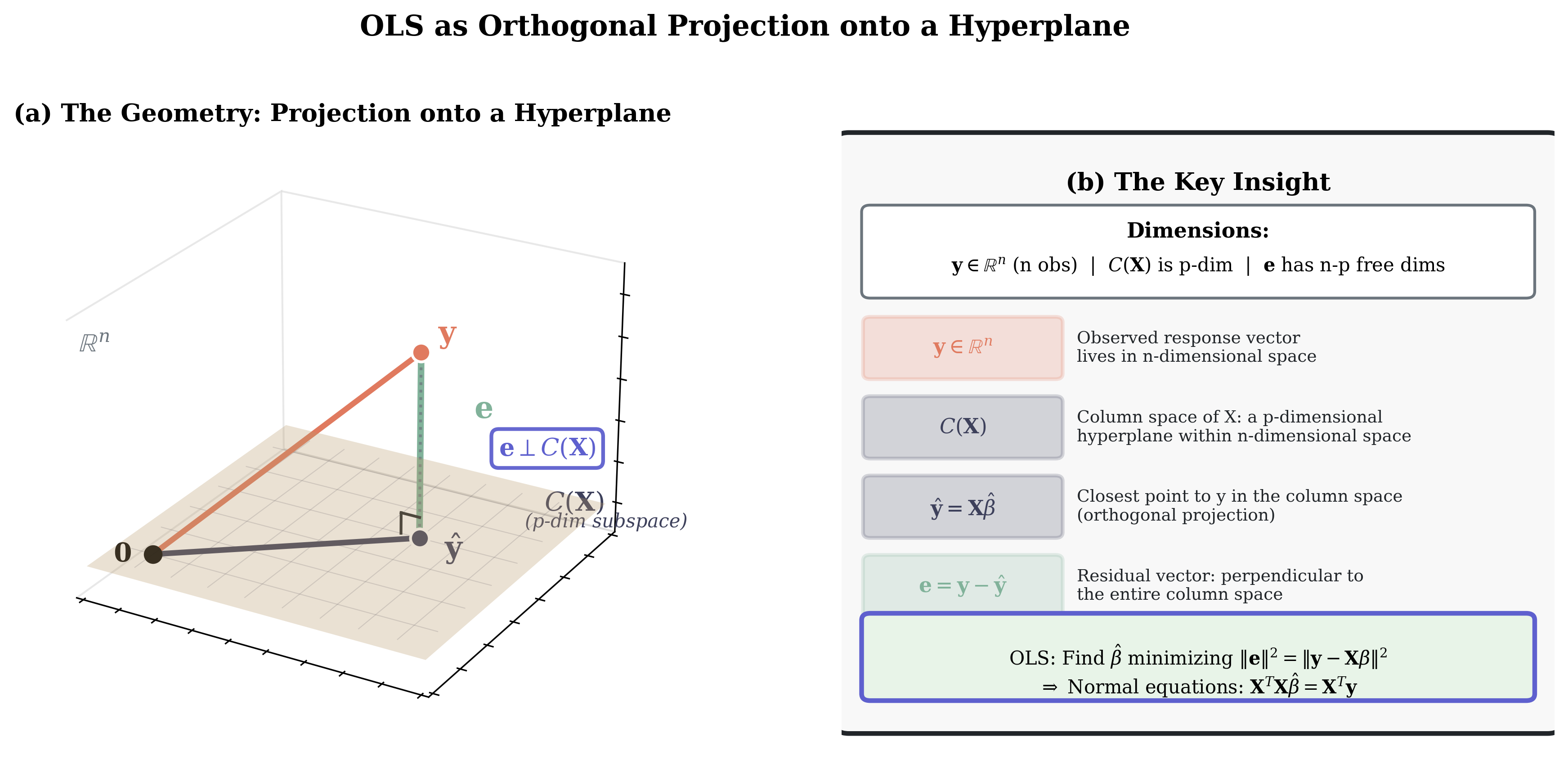
Fig. 82 Figure 3.4.1: OLS as orthogonal projection. The observed \(\mathbf{y}\) lives in \(\mathbb{R}^n\), while the column space \(\mathcal{C}(\mathbf{X})\) is a p-dimensional hyperplane. The fitted values \(\hat{\mathbf{y}} = \mathbf{X}\hat{\boldsymbol{\beta}}\) are the closest point to \(\mathbf{y}\) in this subspace. The residual \(\mathbf{e} = \mathbf{y} - \hat{\mathbf{y}}\) is perpendicular to the entire column space.
The Orthogonality Principle
The closest point to \(\mathbf{y}\) in a subspace is the orthogonal projection. The projection \(\hat{\mathbf{y}}\) satisfies:
This means the residual \(\mathbf{e} = \mathbf{y} - \hat{\mathbf{y}}\) is orthogonal to every vector in the column space. Since any vector in \(\mathcal{C}(\mathbf{X})\) can be written as \(\mathbf{X}\mathbf{a}\) for some \(\mathbf{a} \in \mathbb{R}^p\):
This requires:
The only way this holds for all \(\mathbf{a}\) is if:
Rearranging:
We’ve recovered the normal equations (55) geometrically! The name “normal equations” now makes sense: they express that residuals are normal (perpendicular) to the column space.
The Hat Matrix
The hat matrix (or projection matrix) projects \(\mathbf{y}\) onto \(\mathcal{C}(\mathbf{X})\):
The fitted values are:
The name “hat matrix” comes from putting a hat on \(\mathbf{y}\) to get \(\hat{\mathbf{y}}\).
Properties of the hat matrix:
Symmetric: \(\mathbf{H}^\top = \mathbf{H}\)
Proof: \(\mathbf{H}^\top = [\mathbf{X}(\mathbf{X}^\top\mathbf{X})^{-1}\mathbf{X}^\top]^\top = \mathbf{X}[(\mathbf{X}^\top\mathbf{X})^{-1}]^\top\mathbf{X}^\top = \mathbf{X}(\mathbf{X}^\top\mathbf{X})^{-1}\mathbf{X}^\top = \mathbf{H}\)
Idempotent: \(\mathbf{H}^2 = \mathbf{H}\) (projecting twice gives the same result)
Proof: \(\mathbf{H}^2 = \mathbf{X}(\mathbf{X}^\top\mathbf{X})^{-1}\mathbf{X}^\top \mathbf{X}(\mathbf{X}^\top\mathbf{X})^{-1}\mathbf{X}^\top = \mathbf{X}(\mathbf{X}^\top\mathbf{X})^{-1}\mathbf{X}^\top = \mathbf{H}\)
Trace: \(\text{tr}(\mathbf{H}) = p\)
Proof: Using \(\text{tr}(\mathbf{AB}) = \text{tr}(\mathbf{BA})\): \(\text{tr}(\mathbf{H}) = \text{tr}(\mathbf{X}(\mathbf{X}^\top\mathbf{X})^{-1}\mathbf{X}^\top) = \text{tr}((\mathbf{X}^\top\mathbf{X})^{-1}\mathbf{X}^\top\mathbf{X}) = \text{tr}(\mathbf{I}_p) = p\)
Leverage: The diagonal elements \(h_{ii} \in [0, 1]\) of the hat matrix (58) measure how much observation \(i\) influences its own fitted value.
The residual vector can also be written using a projection matrix:
where \(\mathbf{M} = \mathbf{I} - \mathbf{H}\) projects onto the orthogonal complement of \(\mathcal{C}(\mathbf{X})\).
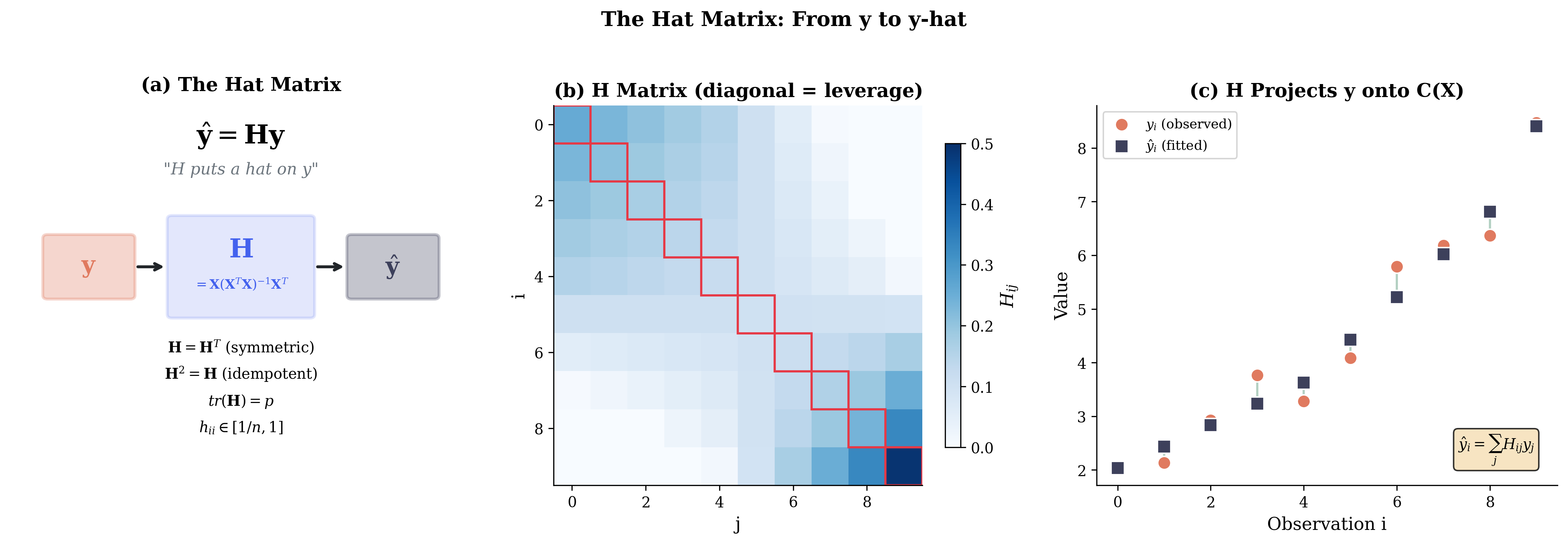
Fig. 83 Figure 3.4.3: The hat matrix \(\mathbf{H} = \mathbf{X}(\mathbf{X}^\top\mathbf{X})^{-1}\mathbf{X}^\top\) “puts a hat on y.” (a) Conceptual view: H transforms observed y into fitted ŷ. (b) Matrix visualization showing larger diagonal elements (leverage) for extreme observations. (c) The projection: H maps each \(y_i\) to \(\hat{y}_i\).
Rank, Pseudo-Inverse, and When Solutions Exist
When \(\mathbf{X}\) has full column rank (\(\text{rank}(\mathbf{X}) = p\)), the solution is unique:
The matrix \((\mathbf{X}^\top\mathbf{X})^{-1}\mathbf{X}^\top\) is the left pseudo-inverse of \(\mathbf{X}\), denoted \(\mathbf{X}^+\). It satisfies \(\mathbf{X}^+\mathbf{X} = \mathbf{I}_p\).
What if \(\mathbf{X}\) doesn’t have full rank?
When \(\text{rank}(\mathbf{X}) = r < p\) (multicollinearity), \(\mathbf{X}^\top\mathbf{X}\) is singular and not invertible. The normal equations \(\mathbf{X}^\top\mathbf{X}\boldsymbol{\beta} = \mathbf{X}^\top\mathbf{y}\) still have solutions, but infinitely many—the solution set is a \((p-r)\)-dimensional affine subspace.
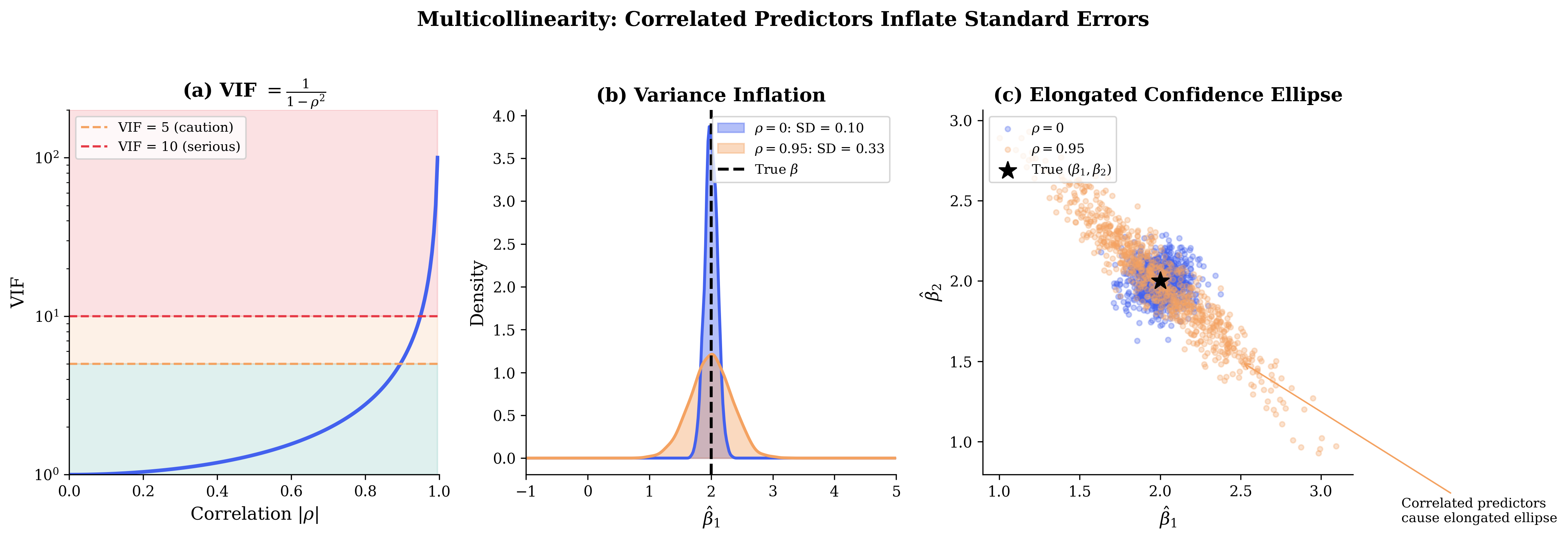
Fig. 84 Figure 3.4.12: Multicollinearity inflates standard errors. (a) VIF grows rapidly as correlation approaches 1: \(\text{VIF} = 1/(1-\rho^2)\). (b) With high correlation (\(\rho = 0.95\)), the sampling distribution of \(\hat{\beta}_1\) is much wider than with uncorrelated predictors. (c) The joint confidence region becomes an elongated ellipse when predictors are correlated.
In this case, we use the Moore-Penrose pseudo-inverse \(\mathbf{X}^+\), which selects the minimum-norm solution:
This solution has the smallest \(\|\boldsymbol{\beta}\|\) among all solutions to the normal equations.
In practice: Software like numpy.linalg.lstsq and scipy.linalg.lstsq use SVD-based methods that handle rank deficiency automatically. (Rank and the singular value decomposition are reviewed in Appendix B.)
import numpy as np

# Example with exact multicollinearity
# x3 = x1 + x2 (perfect linear dependence)
X_singular = np.array([
    [1, 1, 0, 1],
    [1, 0, 1, 1],
    [1, 2, 1, 3],
    [1, 1, 2, 3]
])
y = np.array([1, 2, 4, 5])

# Check rank
print(f"Matrix shape: {X_singular.shape}")
print(f"Rank: {np.linalg.matrix_rank(X_singular)}")
print(f"X'X is singular: {np.linalg.det(X_singular.T @ X_singular) == 0}")

# lstsq handles rank deficiency via SVD
beta_hat, residuals, rank, s = np.linalg.lstsq(X_singular, y, rcond=None)
print(f"\nMinimum-norm solution: {beta_hat}")
print(f"Singular values: {s}")
Matrix shape: (4, 4)
Rank: 3
X'X is singular: True

Minimum-norm solution: [9.32295354e-16 2.22044605e-16 1.00000000e+00 1.00000000e+00]
Singular values: [5.76877982 1.41421356 0.84922282 0.        ]
Properties of the OLS Estimator
Having derived the OLS estimator, we now examine its statistical properties.
Convention: Fixed Design
Throughout this section, we treat \(\mathbf{X}\) as fixed (non-random) and condition all statements on \(\mathbf{X}\). Expectations, variances, and distributions are conditional on \(\mathbf{X}\). This “fixed design” viewpoint is standard in classical regression theory. When \(\mathbf{X}\) is random, results hold conditional on the observed \(\mathbf{X}\).
Unbiasedness
Theorem: OLS is Unbiased
Under assumptions GM1-GM3, the OLS estimator is unbiased:
Proof:
Starting from the OLS estimator (56) and substituting \(\mathbf{y} = \mathbf{X}\boldsymbol{\beta} + \boldsymbol{\varepsilon}\):
Taking expectations conditional on \(\mathbf{X}\):
where we used GM3: \(\mathbb{E}[\boldsymbol{\varepsilon} | \mathbf{X}] = \mathbf{0}\). ∎
Variance-Covariance Matrix
Theorem: Variance of OLS Estimator
Under assumptions GM1-GM4:
Proof:
From above, \(\hat{\boldsymbol{\beta}} - \boldsymbol{\beta} = (\mathbf{X}^\top\mathbf{X})^{-1}\mathbf{X}^\top\boldsymbol{\varepsilon}\).
Let \(\mathbf{A} = (\mathbf{X}^\top\mathbf{X})^{-1}\mathbf{X}^\top\). Then:
Now compute \(\mathbf{A}\mathbf{A}^\top\):
Therefore:
∎
Interpreting the variance formula (59):
The variance of the \(j\)-th coefficient is:
The theoretical standard deviation is:
In practice, we replace \(\sigma\) with its estimate \(s\) (see below).
The Gauss-Markov Theorem
The Gauss-Markov theorem is one of the most important results in regression theory. It establishes OLS as the Best Linear Unbiased Estimator (BLUE).
What BLUE Means
Let’s unpack each word:
Estimator: A function of the data that produces an estimate of the parameter
Unbiased: \(\mathbb{E}[\hat{\boldsymbol{\beta}}] = \boldsymbol{\beta}\) (hits the target on average)
Linear: The estimator is a linear function of \(\mathbf{y}\): \(\tilde{\boldsymbol{\beta}} = \mathbf{C}\mathbf{y}\) for some matrix \(\mathbf{C}\)
Best: Has the smallest variance among all linear unbiased estimators
Why focus on linear estimators?
Tractability: Linear estimators have simple variance formulas
Sufficiency: For normal errors, linear estimators can be optimal even among nonlinear ones
Robustness considerations: Nonlinear estimators may be more efficient under specific distributional assumptions but fail badly when those assumptions are wrong
The Theorem Statement
Theorem: Gauss-Markov
Under assumptions GM1-GM4 (linearity, full rank, strict exogeneity, spherical errors), the OLS estimator \(\hat{\boldsymbol{\beta}} = (\mathbf{X}^\top\mathbf{X})^{-1}\mathbf{X}^\top\mathbf{y}\) is BLUE:
For any other linear unbiased estimator \(\tilde{\boldsymbol{\beta}} = \mathbf{C}\mathbf{y}\) of \(\boldsymbol{\beta}\):
In particular, for any coefficient:
OLS achieves the minimum variance among all linear unbiased estimators.
Complete Proof
Step 1: Characterize linear unbiased estimators
Any linear estimator has the form \(\tilde{\boldsymbol{\beta}} = \mathbf{C}\mathbf{y}\) for some \(p \times n\) matrix \(\mathbf{C}\).
For \(\tilde{\boldsymbol{\beta}}\) to be unbiased:
This requires \(\mathbf{C}\mathbf{X} = \mathbf{I}_p\).
Step 2: Write any linear unbiased estimator as OLS plus something
Let \(\mathbf{A} = (\mathbf{X}^\top\mathbf{X})^{-1}\mathbf{X}^\top\) be the OLS matrix, so \(\hat{\boldsymbol{\beta}} = \mathbf{A}\mathbf{y}\).
Define \(\mathbf{D} = \mathbf{C} - \mathbf{A}\). Then any linear unbiased estimator can be written:
Since both \(\mathbf{C}\) and \(\mathbf{A}\) satisfy \(\mathbf{C}\mathbf{X} = \mathbf{I}_p\) and \(\mathbf{A}\mathbf{X} = \mathbf{I}_p\):
Step 3: Compute the variance of the alternative estimator
Conditional on \(\mathbf{X}\), the variance of any linear estimator \(\tilde{\boldsymbol{\beta}} = \mathbf{C}\mathbf{y}\) is:
Step 4: Show the cross-terms vanish
Compute \(\mathbf{A}\mathbf{D}^\top\):
Now, \(\mathbf{D}\mathbf{X} = \mathbf{0}\) implies \(\mathbf{X}^\top\mathbf{D}^\top = \mathbf{0}\). Therefore:
Similarly, \(\mathbf{D}\mathbf{A}^\top = (\mathbf{A}\mathbf{D}^\top)^\top = \mathbf{0}\).
Step 5: Conclude
Since \(\mathbf{D}\mathbf{D}^\top\) is positive semi-definite (for any \(\mathbf{v}\), \(\mathbf{v}^\top\mathbf{D}\mathbf{D}^\top\mathbf{v} = \|\mathbf{D}^\top\mathbf{v}\|^2 \geq 0\)):
with equality if and only if \(\mathbf{D} = \mathbf{0}\), i.e., \(\tilde{\boldsymbol{\beta}} = \hat{\boldsymbol{\beta}}\). ∎
What Happens When Assumptions Fail
Each Gauss-Markov assumption is critical. Here’s what breaks when each fails:
Assumption |
Violation Example |
Consequence for OLS |
Remedy |
|---|---|---|---|
GM1 Linearity |
True model is \(y = \beta_0 e^{\beta_1 x} + \varepsilon\) but we fit \(y = \beta_0 + \beta_1 x\) |
OLS is biased and inconsistent; converges to wrong quantity as \(n \to \infty\) |
Re-specify the model; transform predictors or add polynomial terms if misspecification is mild; nonlinear regression methods are beyond the scope of this chapter |
GM2 Full Rank |
Perfect multicollinearity: \(x_3 = 2x_1 + x_2\) |
\(\mathbf{X}^\top\mathbf{X}\) is singular; OLS estimator not unique |
Remove redundant predictors; use ridge regularization (covered in Regularization: Ridge and LASSO later in this section) |
GM3 Exogeneity |
Excluded variable correlated with included predictor (e.g., omitted confounder) |
Slope estimates biased and inconsistent; a constant nonzero mean in \(\varepsilon\) is absorbed by the intercept and is harmless |
Include the omitted variable if observable; instrumental variables and fixed effects are remedies when it is not (beyond scope of this chapter) |
GM4a Homoskedasticity |
Variance increases with \(x\): \(\text{Var}(\varepsilon_i) = \sigma^2 x_i^2\) |
OLS remains unbiased but standard errors are wrong; \(t\)-tests and CIs have incorrect size |
Robust (sandwich) standard errors (HC0–HC3); covered in Robust Standard Errors later in this section |
GM4b No autocorrelation |
Time series: \(\varepsilon_t = \rho\varepsilon_{t-1} + u_t\) |
OLS remains unbiased but standard errors underestimate variability under positive autocorrelation; \(t\)-tests invalid |
Heteroskedasticity and autocorrelation consistent (HAC) standard errors; GLS and time-series methods are beyond this chapter’s scope |
Common Pitfall ⚠️ Endogeneity
The most serious violation is GM3 (exogeneity): the requirement that \(\mathbb{E}[\varepsilon_i | \mathbf{X}] = 0\) for all \(i\). This “conditional mean zero” condition says that knowing \(\mathbf{X}\) tells you nothing about the expected error.
When \(\mathbb{E}[\varepsilon | \mathbf{X}] \neq \mathbf{0}\):
OLS is biased even in large samples (inconsistent)
No amount of data fixes the problem
Robust standard errors do not help: They correct for heteroskedasticity, not bias. If your coefficients are biased, having more precise standard errors for the wrong value doesn’t help!
Common causes: omitted variables correlated with included predictors, measurement error in \(\mathbf{X}\), simultaneity (reverse causation).
Detection is difficult since we don’t observe \(\varepsilon\). Economic theory, domain knowledge, and careful study design are essential. Remedies include instrumental variables and natural experiments.
Estimating the Error Variance
The variance formula \(\text{Var}(\hat{\boldsymbol{\beta}}) = \sigma^2(\mathbf{X}^\top\mathbf{X})^{-1}\) depends on the unknown \(\sigma^2\). We need to estimate it.
The Residual Sum of Squares
Define the residuals as \(\mathbf{e} = \mathbf{y} - \hat{\mathbf{y}} = \mathbf{y} - \mathbf{X}\hat{\boldsymbol{\beta}}\).
The residual sum of squares (RSS) is:
A natural estimator of \(\sigma^2\) might be \(\text{RSS}/n\). However, this is biased because residuals underestimate the true errors.
The Unbiased Estimator
Theorem: Unbiased Estimator of σ²
Under GM1-GM4:
is an unbiased estimator of \(\sigma^2\): \(\mathbb{E}[s^2] = \sigma^2\).
Proof sketch:
The residuals can be written as \(\mathbf{e} = \mathbf{M}\mathbf{y} = \mathbf{M}(\mathbf{X}\boldsymbol{\beta} + \boldsymbol{\varepsilon}) = \mathbf{M}\boldsymbol{\varepsilon}\) where \(\mathbf{M} = \mathbf{I} - \mathbf{H}\).
(Note: \(\mathbf{M}\mathbf{X}\boldsymbol{\beta} = (\mathbf{I} - \mathbf{H})\mathbf{X}\boldsymbol{\beta} = \mathbf{X}\boldsymbol{\beta} - \mathbf{X}(\mathbf{X}^\top\mathbf{X})^{-1}\mathbf{X}^\top\mathbf{X}\boldsymbol{\beta} = \mathbf{X}\boldsymbol{\beta} - \mathbf{X}\boldsymbol{\beta} = \mathbf{0}\))
Then:
since \(\mathbf{M}\) is idempotent (\(\mathbf{M}^2 = \mathbf{M}\)) and symmetric.
Taking expectations and using the trace formula for quadratic forms:
Since \(\text{tr}(\mathbf{M}) = \text{tr}(\mathbf{I} - \mathbf{H}) = n - \text{tr}(\mathbf{H}) = n - p\):
Therefore \(\mathbb{E}[\text{RSS}/(n-p)] = \sigma^2\). ∎
Degrees of freedom interpretation: We estimate \(p\) parameters from \(n\) observations, leaving \(n - p\) degrees of freedom for estimating error variance.
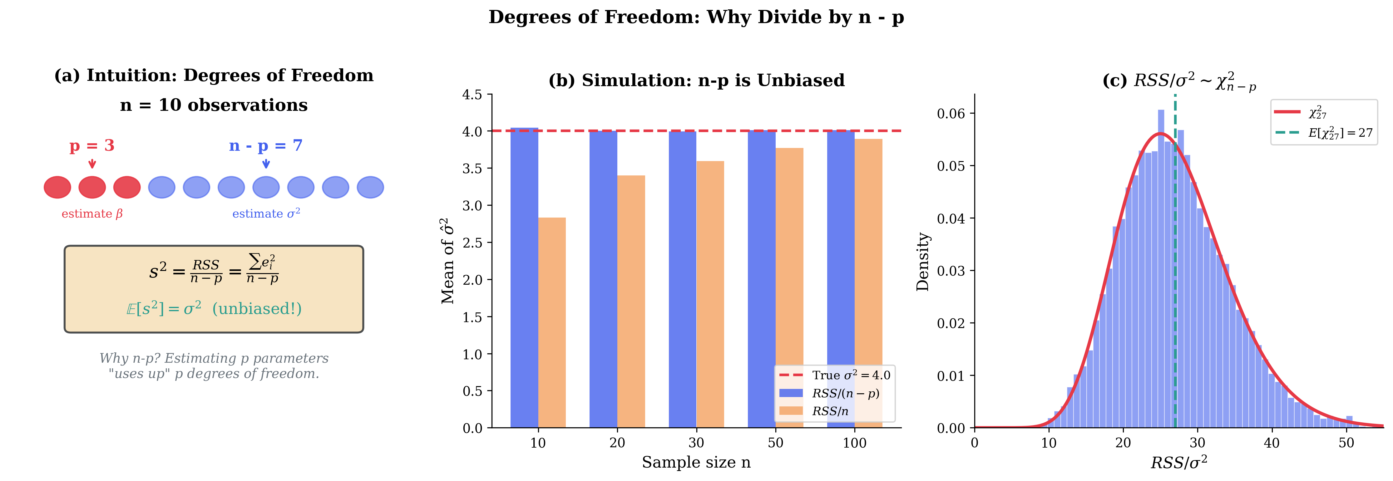
Fig. 85 Figure 3.4.5: Degrees of freedom explained. (a) With n observations, p are “used up” estimating \(\boldsymbol{\beta}\), leaving n-p to estimate \(\sigma^2\). (b) Simulation confirms \(s^2 = \text{RSS}/(n-p)\) is unbiased while \(\text{RSS}/n\) underestimates \(\sigma^2\). (c) Under normality, \(\text{RSS}/\sigma^2 \sim \chi^2_{n-p}\).
Standard Errors of Coefficients
The estimated variance-covariance matrix of \(\hat{\boldsymbol{\beta}}\) is:
The standard error of the \(j\)-th coefficient is:
import numpy as np
from scipy import stats

def ols_with_inference(X, y):
    """
    Perform OLS regression with inference.

    Note: This function uses explicit matrix formulas for pedagogical clarity.
    For production code, use np.linalg.lstsq() or scipy.linalg.lstsq() which
    are numerically more stable (see Numerical Stability section).

    Returns
    -------
    dict with beta_hat, se, t_stats, p_values, R2, s2
    """
    n, p = X.shape

    # OLS estimates (formula-aligned; use np.linalg.lstsq for production)
    XtX = X.T @ X
    XtX_inv = np.linalg.inv(XtX)  # Needed for standard errors
    beta_hat = np.linalg.solve(XtX, X.T @ y)  # More stable than inv() @ y

    # Fitted values and residuals
    y_hat = X @ beta_hat
    residuals = y - y_hat

    # Variance estimation
    RSS = residuals @ residuals
    s2 = RSS / (n - p)
    s = np.sqrt(s2)

    # Standard errors
    var_beta = s2 * XtX_inv
    se = np.sqrt(np.diag(var_beta))

    # t-statistics and p-values
    t_stats = beta_hat / se
    p_values = 2 * (1 - stats.t.cdf(np.abs(t_stats), df=n-p))

    # R-squared
    TSS = np.sum((y - np.mean(y))**2)
    R2 = 1 - RSS / TSS
    R2_adj = 1 - (1 - R2) * (n - 1) / (n - p)

    return {
        'beta_hat': beta_hat,
        'se': se,
        't_stats': t_stats,
        'p_values': p_values,
        'R2': R2,
        'R2_adj': R2_adj,
        's2': s2,
        's': s,
        'residuals': residuals,
        'y_hat': y_hat
    }

# Example: mtcars-style data
rng = np.random.default_rng(42)
n = 32
hp = rng.uniform(50, 300, n)  # horsepower
wt = rng.uniform(1.5, 5.5, n)  # weight (1000 lbs)
mpg = 40 - 0.03 * hp - 4 * wt + rng.normal(0, 2, n)

X = np.column_stack([np.ones(n), hp, wt])
y = mpg

results = ols_with_inference(X, y)

print("="*60)
print("OLS REGRESSION RESULTS")
print("="*60)
print(f"\nSample size: n = {n}, Predictors: p = {X.shape[1]}")
print(f"R² = {results['R2']:.4f}, Adjusted R² = {results['R2_adj']:.4f}")
print(f"Residual SE: s = {results['s']:.4f}")

print(f"\n{'Coefficient':<12} {'Estimate':>10} {'Std Error':>10} {'t-stat':>10} {'p-value':>10}")
print("-"*54)
names = ['Intercept', 'hp', 'wt']
for name, b, se, t, p in zip(names, results['beta_hat'], results['se'],
                               results['t_stats'], results['p_values']):
    print(f"{name:<12} {b:>10.4f} {se:>10.4f} {t:>10.2f} {p:>10.4f}")
============================================================
OLS REGRESSION RESULTS
============================================================

Sample size: n = 32, Predictors: p = 3
R² = 0.9520, Adjusted R² = 0.9486
Residual SE: s = 1.2165

Coefficient    Estimate  Std Error     t-stat    p-value
------------------------------------------------------
Intercept       40.3548     0.8585      47.01     0.0000
hp              -0.0265     0.0031      -8.61     0.0000
wt              -4.3206     0.2290     -18.87     0.0000
Distributional Results Under Normality
Under the full normal linear model (GM1-GM5), we have exact distributional results enabling precise inference.
Distribution of the OLS Estimator
Theorem: Normality of OLS
Under GM1-GM5:
Proof: Since \(\hat{\boldsymbol{\beta}} = (\mathbf{X}^\top\mathbf{X})^{-1}\mathbf{X}^\top\mathbf{y}\) and \(\mathbf{y} = \mathbf{X}\boldsymbol{\beta} + \boldsymbol{\varepsilon}\) with \(\boldsymbol{\varepsilon} \sim \mathcal{N}(\mathbf{0}, \sigma^2\mathbf{I})\):
\(\hat{\boldsymbol{\beta}}\) is a linear transformation of normal \(\boldsymbol{\varepsilon}\), hence normal. Mean and variance computed earlier. ∎
Distribution of s²
Theorem: Chi-Square Distribution of RSS
Under GM1-GM5:
Moreover, \(s^2\) and \(\hat{\boldsymbol{\beta}}\) are independent.
Proof sketch: RSS can be written as \(\boldsymbol{\varepsilon}^\top\mathbf{M}\boldsymbol{\varepsilon}/\sigma^2\) where \(\mathbf{M} = \mathbf{I} - \mathbf{H}\) is idempotent with rank \(n - p\). By Cochran’s theorem, this is \(\chi^2_{n-p}\).
The independence follows from the fact that \(\hat{\boldsymbol{\beta}}\) depends on \(\boldsymbol{\varepsilon}\) through \((\mathbf{X}^\top\mathbf{X})^{-1}\mathbf{X}^\top\boldsymbol{\varepsilon}\) and \(s^2\) through \(\mathbf{M}\boldsymbol{\varepsilon}\). Since \((\mathbf{X}^\top\mathbf{X})^{-1}\mathbf{X}^\top \cdot \sigma^2 \mathbf{M} = \mathbf{0}\) (orthogonality), these linear forms of a multivariate normal are independent. ∎
t-Tests for Individual Coefficients
Combining the above results:
This enables t-tests for individual coefficients:
Null hypothesis: \(H_0: \beta_j = \beta_{j,0}\) (often \(\beta_{j,0} = 0\))
Test statistic: \(t = \frac{\hat{\beta}_j - \beta_{j,0}}{\text{SE}(\hat{\beta}_j)}\)
Decision: Reject at level \(\alpha\) if \(|t| > t_{n-p, 1-\alpha/2}\)
Confidence interval for \(\beta_j\):
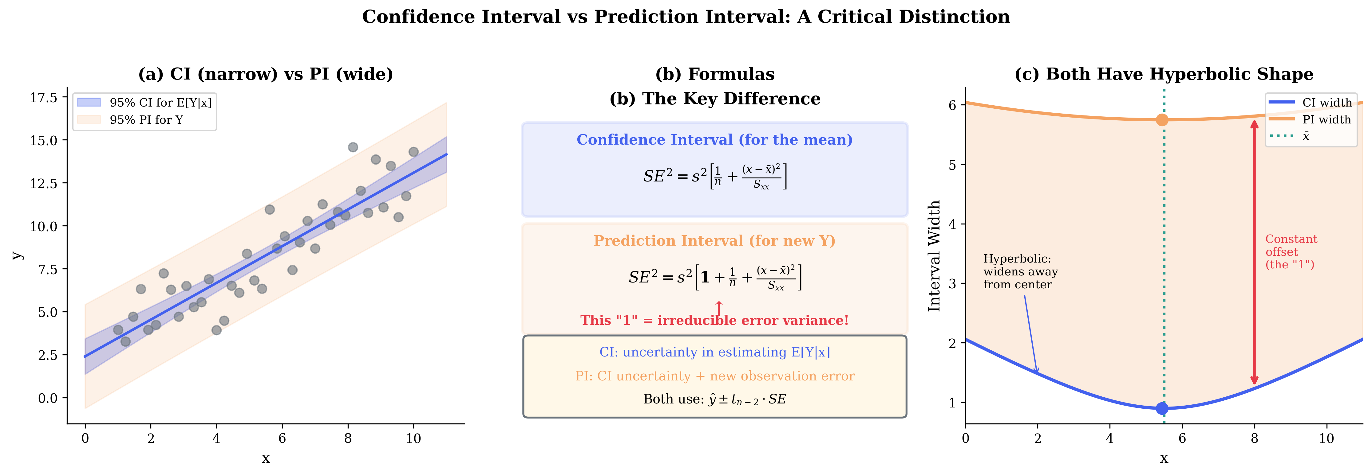
Fig. 86 Figure 3.4.7: Confidence interval (for the mean) vs. prediction interval (for new Y). (a) The CI (narrow band) captures uncertainty in \(E[Y|x]\), while the PI (wide band) also includes the irreducible error variance. (b) The formulas differ by the “1” inside the square root—representing \(\sigma^2\) for a new observation. (c) Both intervals have hyperbolic shape, widening away from \(\bar{x}\), but the PI is offset by a constant amount.
F-Tests for Nested Models
To test whether a subset of coefficients is jointly zero, use the F-test.
Setup: Compare: - Restricted model (R): \(q\) constraints, \(\text{RSS}_R\) - Full model (F): no constraints, \(\text{RSS}_F\)
Theorem: F-Test for Nested Models
Under \(H_0\) (constraints are true) and normality:
Example: Testing \(H_0: \beta_2 = \beta_3 = 0\) (joint significance of two predictors).
import numpy as np
from scipy import stats

def f_test_nested(y, X_full, X_reduced):
    """
    F-test comparing full model to reduced (nested) model.
    """
    n = len(y)
    p_full = X_full.shape[1]
    p_reduced = X_reduced.shape[1]
    q = p_full - p_reduced  # number of restrictions

    # Fit both models
    beta_full = np.linalg.lstsq(X_full, y, rcond=None)[0]
    beta_reduced = np.linalg.lstsq(X_reduced, y, rcond=None)[0]

    RSS_full = np.sum((y - X_full @ beta_full)**2)
    RSS_reduced = np.sum((y - X_reduced @ beta_reduced)**2)

    # F statistic
    F = ((RSS_reduced - RSS_full) / q) / (RSS_full / (n - p_full))
    p_value = 1 - stats.f.cdf(F, q, n - p_full)

    return {'F': F, 'df1': q, 'df2': n - p_full, 'p_value': p_value,
            'RSS_full': RSS_full, 'RSS_reduced': RSS_reduced}

# Example: test if both hp and wt are needed
X_full = np.column_stack([np.ones(n), hp, wt])
X_reduced = np.column_stack([np.ones(n)])  # intercept only

result = f_test_nested(y, X_full, X_reduced)
print(f"\nF-test: Are hp and wt jointly significant?")
print(f"F({result['df1']}, {result['df2']}) = {result['F']:.2f}")
print(f"p-value = {result['p_value']:.6f}")
Example 💡 OLS Inference on the Advertising Data
Given: The ISLR Advertising data (\(n = 200\) markets), regressing Sales
on the three media budgets TV, Radio, and Newspaper. A single fitted model
exercises the whole inference toolkit of this section—the individual t-tests, the joint
F-test, and the \(F = t^2\) identity.
Find: Which predictors carry their weight once the others are held fixed?
import pandas as pd
import statsmodels.formula.api as smf

url = ("https://pqyjaywwccbnqpwgeiuv.supabase.co/storage/v1/object/"
       "public/STAT%20418%20Images/Data/Chapter3/Advertising.csv")
adv = pd.read_csv(url)

full = smf.ols("Sales ~ TV + Radio + Newspaper", data=adv).fit()
print(f"Full model  Sales ~ TV + Radio + Newspaper   (n = {int(full.nobs)})")
print(f"  R^2 = {full.rsquared:.3f}   overall F = {full.fvalue:.1f}")

print("\nIndividual t-tests  (H0: beta_j = 0):")
for v in ["TV", "Radio", "Newspaper"]:
    print(f"  {v:10s} coef={full.params[v]:+.4f}  t={full.tvalues[v]:+.2f}  p={full.pvalues[v]:.3f}")

# Joint F-test: are Radio and Newspaper jointly unnecessary?
joint = full.f_test("Radio = 0, Newspaper = 0")
print(f"\nJoint F-test  H0: beta_Radio = beta_Newspaper = 0:")
print(f"  F = {float(joint.fvalue):.1f}  (df {int(joint.df_num)}, {int(joint.df_denom)})  p = {float(joint.pvalue):.1e}")

# Single restriction reproduces the t-test: F = t^2
drop_news = full.f_test("Newspaper = 0")
print(f"\nSingle restriction  H0: beta_Newspaper = 0:")
print(f"  F = {float(drop_news.fvalue):.3f}  = t^2 = {full.tvalues['Newspaper']**2:.3f}")

# Newspaper alone tells a different story (confounding via Radio)
simple_news = smf.ols("Sales ~ Newspaper", data=adv).fit()
print(f"\nNewspaper ALONE: t = {simple_news.tvalues['Newspaper']:.2f}, "
      f"p = {simple_news.pvalues['Newspaper']:.3f}")
print(f"corr(Radio, Newspaper) = {adv['Radio'].corr(adv['Newspaper']):.3f}")
Output:
Full model  Sales ~ TV + Radio + Newspaper   (n = 200)
  R^2 = 0.897   overall F = 570.3

Individual t-tests  (H0: beta_j = 0):
  TV         coef=+0.0458  t=+32.81  p=0.000
  Radio      coef=+0.1885  t=+21.89  p=0.000
  Newspaper  coef=-0.0010  t=-0.18  p=0.860

Joint F-test  H0: beta_Radio = beta_Newspaper = 0:
  F = 272.0  (df 2, 196)  p = 2.8e-57

Single restriction  H0: beta_Newspaper = 0:
  F = 0.031  = t^2 = 0.031

Newspaper ALONE: t = 3.30, p = 0.001
corr(Radio, Newspaper) = 0.354
The individual t-tests flag TV (\(t = 32.8\)) and Radio (\(t = 21.9\))
as overwhelmingly significant, while Newspaper fails to reject (\(t = -0.18\),
\(p = 0.86\)): with TV and radio already in the model, newspaper spending adds nothing.
The joint F-test that both radio and newspaper are unnecessary is decisively rejected
(\(F = 272\) on \((2, 196)\) df), so the model clearly needs more than TV alone.
The single-restriction F-test for newspaper returns \(F = 0.031\), exactly the square
of its t-statistic (\((-0.18)^2\))—the \(F = t^2\) identity, since a one-coefficient
F-test and the corresponding two-sided t-test are the same test. Finally, a cautionary
twist: regressed alone, Newspaper looks significant (\(t = 3.30\),
\(p = 0.001\)), because newspaper budgets are correlated with radio budgets
(\(r = 0.35\)); once radio is held fixed, newspaper’s apparent effect evaporates. This
is exactly why a multiple-regression coefficient must be read as an effect holding the
other predictors fixed.
Diagnostics and Model Checking
The validity of regression inference depends on assumptions. Diagnostics help detect violations.
Residual Analysis
Types of residuals:
Raw residuals: \(e_i = y_i - \hat{y}_i\)
Standardized residuals: \(r_i = \frac{e_i}{s\sqrt{1 - h_{ii}}}\)
These have approximately constant variance under homoskedasticity.
Studentized (externally): \(t_i = \frac{e_i}{s_{(i)}\sqrt{1 - h_{ii}}} \sim t_{n-p-1}\)
where \(s_{(i)}\) is computed without observation \(i\). Follows exact t-distribution.
Diagnostic plots:
Residuals vs. Fitted: Check linearity (should be random scatter) and homoskedasticity (constant spread)
Q-Q plot of residuals: Check normality (should follow 45° line)
Residuals vs. each predictor: Check functional form
Scale-Location plot: \(\sqrt{|r_i|}\) vs. fitted for homoskedasticity
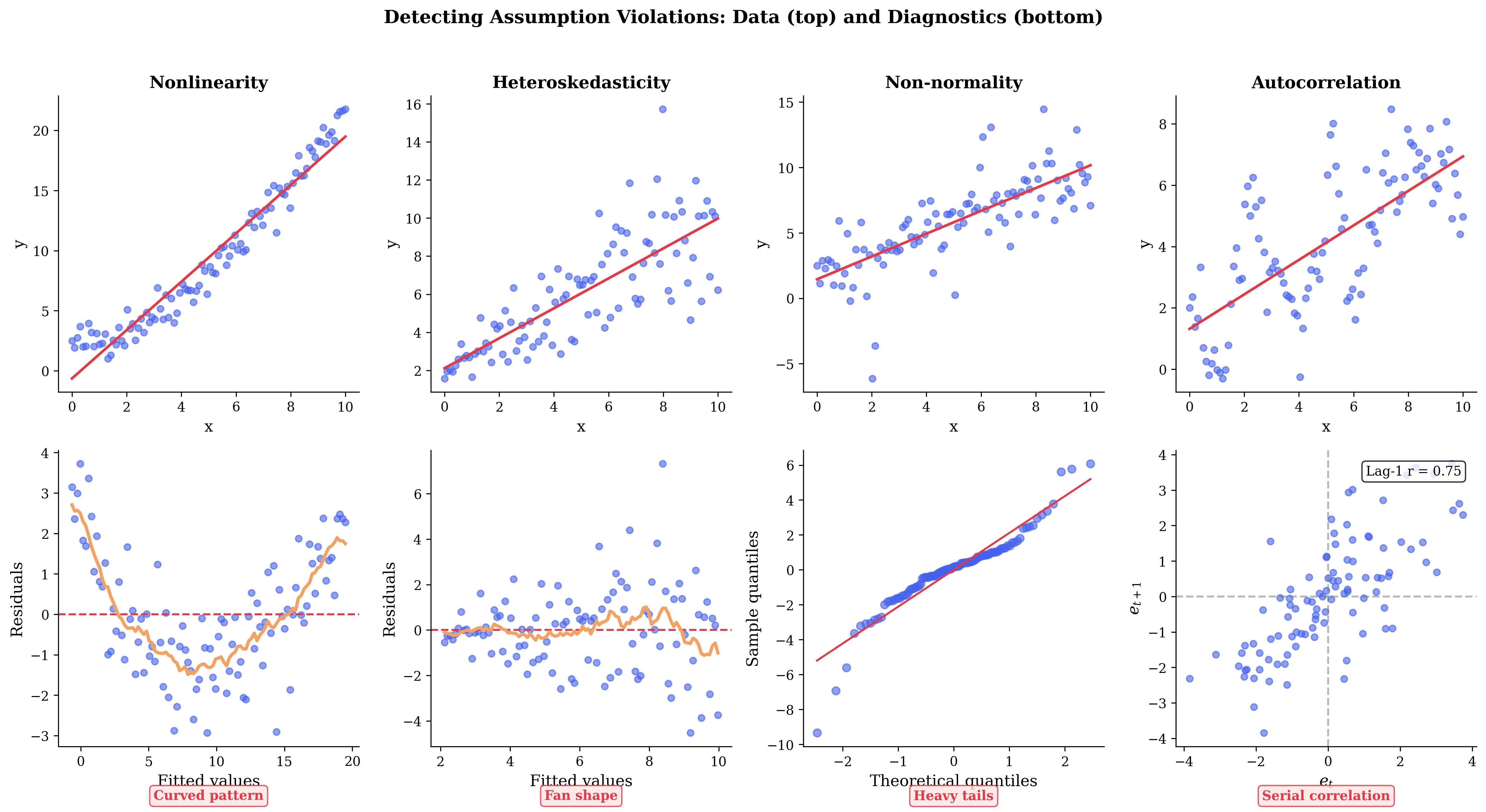
Fig. 87 Figure 3.4.6: Assumption violations gallery. Top: data patterns; Bottom: diagnostic plots. Nonlinearity shows curved residual pattern. Heteroskedasticity produces a fan shape. Non-normality creates heavy tails in Q-Q plots. Autocorrelation shows serial correlation in \(e_t\) vs \(e_{t+1}\) plots.
Leverage and Influence
Not all observations affect the fit equally.
Leverage: \(h_{ii} = [\mathbf{H}]_{ii}\) measures how far \(\mathbf{x}_i\) is from the center of the predictor space.
\(h_{ii} \in [1/n, 1]\) (from idempotence and hat matrix properties)
Average leverage: \(\bar{h} = p/n\)
High leverage if \(h_{ii} > 2p/n\) or \(> 3p/n\)
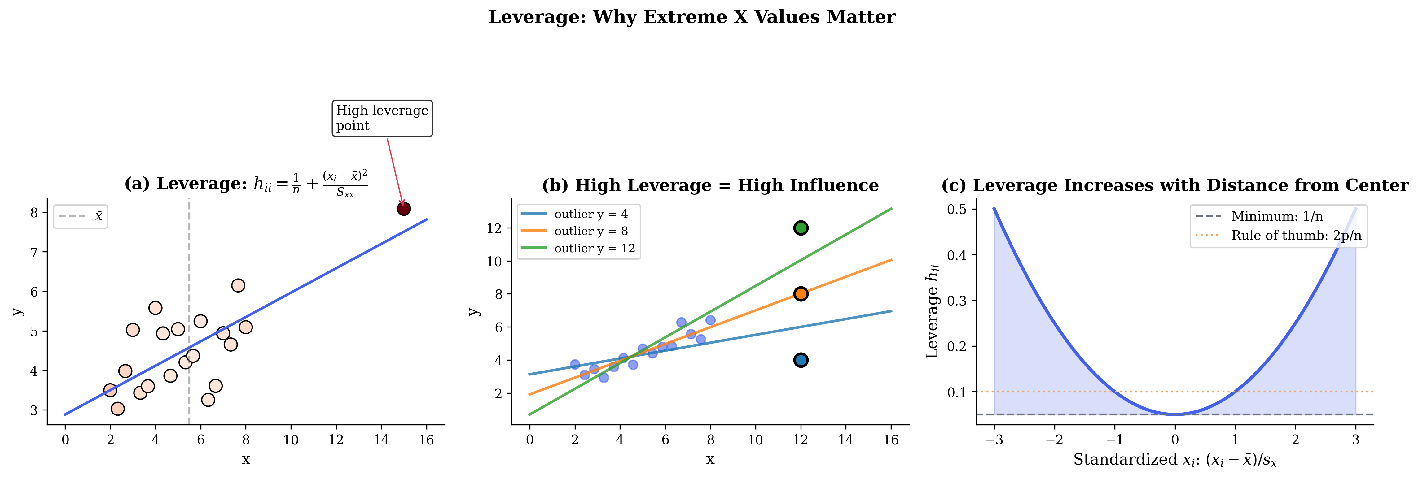
Fig. 88 Figure 3.4.4: Leverage measures how far observation \(x_i\) is from \(\bar{x}\). (a) Points far from center have high leverage (red = high, blue = low). (b) High-leverage points can dramatically influence the regression line. (c) The leverage formula \(h_{ii} = 1/n + (x_i - \bar{x})^2/S_{xx}\) is U-shaped in \(x\).
Influence measures:
Cook’s Distance: Combines leverage and residual size
\[D_i = \frac{r_i^2}{p} \cdot \frac{h_{ii}}{1 - h_{ii}}\]Large if \(D_i > 4/n\) or \(> 1\)
DFFITS: Scaled difference in fitted value when \(i\) deleted
DFBETAS: Change in each coefficient when \(i\) deleted
Robust Standard Errors
When homoskedasticity fails but we still want valid inference, use robust (sandwich) standard errors:
where \(\hat{\boldsymbol{\Omega}} = \text{diag}(e_1^2, \ldots, e_n^2)\) estimates the heteroskedastic structure.
HC variants (heteroskedasticity-consistent):
HC0: \(\hat{\Omega}_{ii} = e_i^2\) (White’s original)
HC1: \(\hat{\Omega}_{ii} = \frac{n}{n-p} e_i^2\) (degrees-of-freedom correction)
HC2: \(\hat{\Omega}_{ii} = \frac{e_i^2}{1 - h_{ii}}\) (leverage adjustment)
HC3: \(\hat{\Omega}_{ii} = \frac{e_i^2}{(1 - h_{ii})^2}\) (jackknife-like, best for small samples)
def robust_se(X, residuals, hc_type='HC1'):
    """
    Compute heteroskedasticity-robust standard errors.

    Note: This implementation forms the full n×n hat matrix H, which is
    O(n²) in memory and time. For large n, compute leverages h_ii directly
    without forming H: h_ii = x_i' (X'X)^{-1} x_i for each row.

    Parameters
    ----------
    X : array, shape (n, p)
        Design matrix
    residuals : array, shape (n,)
        OLS residuals
    hc_type : str
        'HC0', 'HC1', 'HC2', or 'HC3'
    """
    n, p = X.shape
    XtX_inv = np.linalg.inv(X.T @ X)

    # Leverage values (O(n²) - for large n, compute row-by-row instead)
    H = X @ XtX_inv @ X.T
    h = np.diag(H)

    # Construct Omega based on HC type
    e2 = residuals**2
    if hc_type == 'HC0':
        omega = e2
    elif hc_type == 'HC1':
        omega = e2 * n / (n - p)
    elif hc_type == 'HC2':
        omega = e2 / (1 - h)
    elif hc_type == 'HC3':
        omega = e2 / (1 - h)**2
    else:
        raise ValueError(f"Unknown HC type: {hc_type}")

    # Sandwich formula
    meat = X.T @ np.diag(omega) @ X
    sandwich = XtX_inv @ meat @ XtX_inv

    return np.sqrt(np.diag(sandwich))
Bringing It All Together
Linear regression is both a statistical tool and a conceptual framework that illuminates fundamental ideas in inference. We’ve seen:
The calculus approach reveals OLS as the solution to an optimization problem—minimizing squared residuals leads to the normal equations \(\mathbf{X}^\top\mathbf{X}\hat{\boldsymbol{\beta}} = \mathbf{X}^\top\mathbf{y}\).
The geometric approach shows OLS as projection—\(\hat{\mathbf{y}}\) is the orthogonal projection of \(\mathbf{y}\) onto the column space of \(\mathbf{X}\). The residual \(\mathbf{e}\) is perpendicular to all predictors.
The Gauss-Markov theorem establishes that under classical assumptions (linearity, exogeneity, spherical errors), OLS achieves minimum variance among all linear unbiased estimators. This optimality result has driven the dominance of OLS in applied work.
Distributional theory under normality enables exact t-tests and F-tests. Without normality, asymptotic approximations still provide valid inference for large samples.
Diagnostics reveal whether assumptions hold. When they fail, remedies range from robust standard errors to alternative estimators.
Looking Ahead
Section 3.5 extends these ideas to Generalized Linear Models (GLMs)—logistic regression, Poisson regression, and more. GLMs handle non-normal responses while maintaining the interpretability and computational tractability of the linear model framework. The IRLS algorithm for fitting GLMs is essentially Fisher scoring—Newton-Raphson with expected information—applied to the same exponential family likelihoods we met in Section 3.1.
Key Takeaways 📝
Matrix calculus foundation: The gradient of \(\boldsymbol{\beta}^\top\mathbf{A}\boldsymbol{\beta}\) is \(2\mathbf{A}\boldsymbol{\beta}\) (for symmetric \(\mathbf{A}\)), enabling systematic derivation of least squares estimators.
Two perspectives on OLS: Calculus (minimize RSS) and geometry (project onto column space) yield the same normal equations \(\mathbf{X}^\top\mathbf{X}\hat{\boldsymbol{\beta}} = \mathbf{X}^\top\mathbf{y}\).
Gauss-Markov theorem: Under linearity, full rank, exogeneity, and spherical errors, OLS is BLUE—the best linear unbiased estimator. The complete proof uses the \(\mathbf{D}\) matrix decomposition.
Inference requires variance estimation: The unbiased estimator \(s^2 = \text{RSS}/(n-p)\) replaces \(\sigma^2\) in standard error formulas. Under normality, t-tests and F-tests are exact.
Diagnostics are essential: Residual plots, leverage measures, and Cook’s distance detect assumption violations. Robust standard errors (HC0-HC3) provide valid inference under heteroskedasticity.
Outcome alignment: This section addresses Learning Outcomes on implementing regression methods, understanding estimator properties (bias, variance, efficiency), and applying diagnostics—skills essential for Sections 3.5 (GLMs), Chapter 4 (bootstrap for regression), and Chapter 5 (Bayesian linear models).
Numerical Stability: QR Decomposition
The formula \(\hat{\boldsymbol{\beta}} = (\mathbf{X}^\top\mathbf{X})^{-1}\mathbf{X}^\top\mathbf{y}\) is mathematically correct but numerically problematic. Computing \(\mathbf{X}^\top\mathbf{X}\) and inverting it can lose precision due to the condition number. (For background on floating-point arithmetic, machine epsilon, and how condition numbers determine digits lost, see Appendix C.)
The Condition Number Problem
The condition number of a matrix measures sensitivity to numerical errors:
For the product \(\mathbf{X}^\top\mathbf{X}\):
This squaring of the condition number is catastrophic. If \(\mathbf{X}\) has condition number \(10^4\) (not unusual with poorly scaled predictors), then \(\mathbf{X}^\top\mathbf{X}\) has condition number \(10^8\), potentially losing 8 digits of precision.
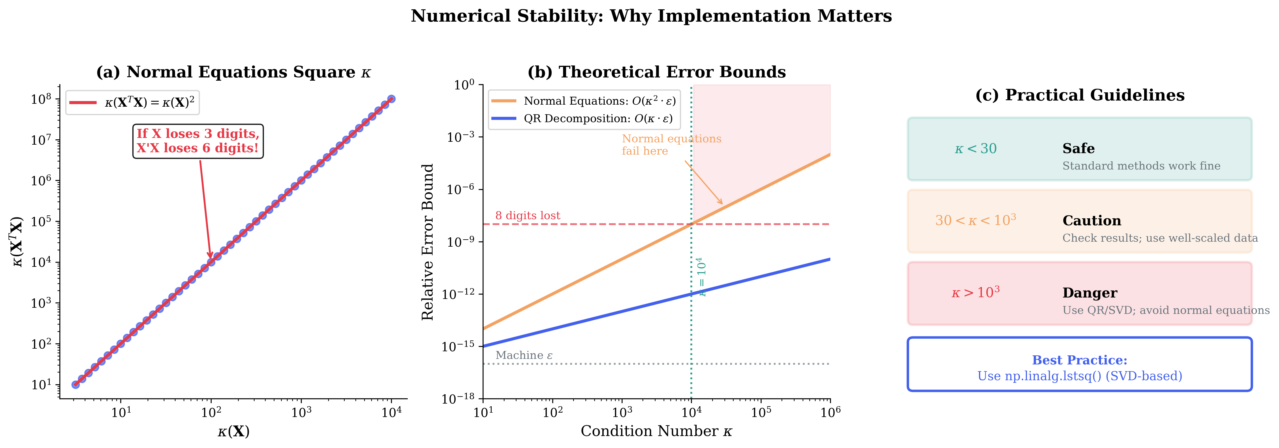
Fig. 89 Figure 3.4.8: Numerical stability matters. (a) Normal equations square the condition number: \(\kappa(\mathbf{X}^\top\mathbf{X}) = \kappa(\mathbf{X})^2\). (b) Theoretical error bounds show QR decomposition with \(O(\kappa \cdot \epsilon)\) error vastly outperforms normal equations with \(O(\kappa^2 \cdot \epsilon)\) error. (c) Practical guidelines: use QR/SVD-based methods (like np.linalg.lstsq) when \(\kappa > 10^3\).
QR Decomposition Solution
The QR decomposition factorizes \(\mathbf{X}\) as:
where:
\(\mathbf{Q} \in \mathbb{R}^{n \times p}\) has orthonormal columns: \(\mathbf{Q}^\top\mathbf{Q} = \mathbf{I}_p\)
\(\mathbf{R} \in \mathbb{R}^{p \times p}\) is upper triangular
Solving the normal equations via QR:
Substitute into \(\mathbf{X}^\top\mathbf{X}\hat{\boldsymbol{\beta}} = \mathbf{X}^\top\mathbf{y}\):
Since \(\mathbf{Q}^\top\mathbf{Q} = \mathbf{I}\) and \(\mathbf{R}^\top\) is invertible:
This triangular system is solved by back-substitution—no matrix inversion needed! (For the QR decomposition itself and the use of triangular solves in place of explicit inversion, see Appendix B.)
Advantages:
Condition number is \(\kappa(\mathbf{R}) = \kappa(\mathbf{X})\), not squared
No explicit computation of \(\mathbf{X}^\top\mathbf{X}\)
Back-substitution is \(O(p^2)\), highly stable
import numpy as np

def ols_qr(X, y):
    """
    Compute OLS via QR decomposition (numerically stable).
    """
    Q, R = np.linalg.qr(X)
    Qty = Q.T @ y
    beta_hat = np.linalg.solve(R, Qty)  # Back-substitution
    return beta_hat

def demonstrate_condition_number():
    """Show the condition number problem."""
    rng = np.random.default_rng(42)
    n = 100

    # Poorly conditioned design matrix (highly correlated predictors)
    x1 = rng.uniform(0, 1, n)
    x2 = x1 + rng.normal(0, 0.0001, n)  # Nearly collinear!

    X = np.column_stack([np.ones(n), x1, x2])
    y = 1 + 2*x1 + 3*x2 + rng.normal(0, 0.1, n)

    # Condition numbers
    kappa_X = np.linalg.cond(X)
    kappa_XtX = np.linalg.cond(X.T @ X)

    print("="*60)
    print("CONDITION NUMBER COMPARISON")
    print("="*60)
    print(f"\nκ(X):     {kappa_X:.2e}")
    print(f"κ(X'X):   {kappa_XtX:.2e}")
    print(f"Ratio:    {kappa_XtX / kappa_X:.2e} (should be ≈ κ(X))")

    # Compare methods
    # Method 1: Normal equations (unstable)
    try:
        beta_normal = np.linalg.solve(X.T @ X, X.T @ y)
        print(f"\nNormal equations: β̂ = {beta_normal}")
    except np.linalg.LinAlgError:
        print("\nNormal equations: FAILED (singular matrix)")

    # Method 2: QR decomposition (stable)
    beta_qr = ols_qr(X, y)
    print(f"QR decomposition: β̂ = {beta_qr}")

    # Method 3: lstsq (uses SVD)
    beta_lstsq = np.linalg.lstsq(X, y, rcond=None)[0]
    print(f"lstsq (SVD):      β̂ = {beta_lstsq}")

demonstrate_condition_number()
============================================================
CONDITION NUMBER COMPARISON
============================================================

κ(X):     1.78e+04
κ(X'X):   3.18e+08
Ratio:    1.78e+04 (should be ≈ κ(X))

Normal equations: β̂ = [  1.0253349  -16.99304398  21.93082782]
QR decomposition: β̂ = [  1.0253349  -16.99304426  21.9308281 ]
lstsq (SVD):      β̂ = [  1.0253349  -16.99304426  21.9308281 ]
Common Pitfall ⚠️ Never Compute (X’X)⁻¹ Explicitly
When writing your own regression code:
Don’t do this:
np.linalg.inv(X.T @ X) @ X.T @ yDo this instead:
np.linalg.lstsq(X, y, rcond=None)[0]
The lstsq function uses SVD internally, which is even more stable than QR and handles rank-deficient matrices gracefully.
Model Selection and Information Criteria
With multiple candidate models, how do we choose? Information criteria balance goodness-of-fit against complexity.
The Bias-Variance Tradeoff
Consider adding a predictor to a model:
RSS decreases (or stays the same)—the fit improves or is unchanged
Variance increases—more parameters to estimate
This is the classic bias-variance tradeoff:
A complex model has low bias (fits the data well) but high variance (overfits to noise). A simple model has higher bias but lower variance.
R-Squared and Adjusted R-Squared
R-squared measures the proportion of variance explained:
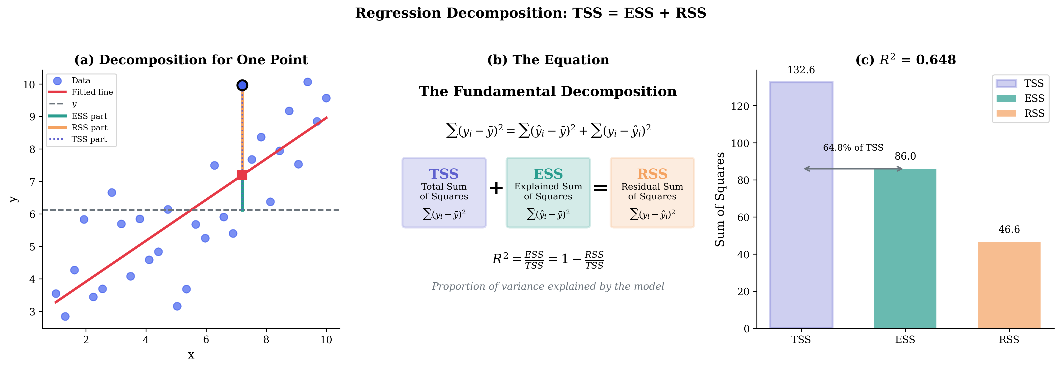
Fig. 90 Figure 3.4.13: The fundamental decomposition TSS = ESS + RSS. (a) For each point, the deviation from \(\bar{y}\) splits into explained (ESS) and residual (RSS) components. (b) The equation: Total Sum of Squares = Explained Sum of Squares + Residual Sum of Squares. (c) \(R^2 = \text{ESS}/\text{TSS}\) is the proportion explained.
Problem: \(R^2\) never decreases when adding predictors, even useless ones.
Adjusted R-squared penalizes for model complexity:
This can decrease when adding a predictor that doesn’t improve the fit enough to justify its inclusion.
Information Criteria
Akaike Information Criterion (AIC):
Bayesian Information Criterion (BIC):
These are the AIC and BIC formulas for Gaussian linear regression, dropping additive constants that cancel when comparing models fit to the same response \(\mathbf{y}\). For general likelihoods, use \(\text{AIC} = -2\ln L + 2p\) and \(\text{BIC} = -2\ln L + p\ln n\).
Both penalize complexity, but BIC penalizes more heavily for large \(n\).
Usage: Lower is better. Compare models by their AIC or BIC values.
Criterion |
Formula |
Penalty |
Best for |
|---|---|---|---|
\(R^2\) |
\(1 - \text{RSS}/\text{TSS}\) |
None (always increases) |
Never for selection |
\(R^2_{\text{adj}}\) |
\(1 - (1-R^2)\frac{n-1}{n-p}\) |
Mild |
Quick comparison |
AIC |
\(n\ln(\text{RSS}/n) + 2p\) |
\(2p\) |
Prediction |
BIC |
\(n\ln(\text{RSS}/n) + p\ln(n)\) |
\(p\ln(n)\) |
Consistent selection |
def model_selection_criteria(y, y_hat, p, n):
    """
    Compute model selection criteria.

    Parameters
    ----------
    y : array
        Observed values
    y_hat : array
        Fitted values
    p : int
        Number of parameters (including intercept)
    n : int
        Sample size
    """
    RSS = np.sum((y - y_hat)**2)
    TSS = np.sum((y - np.mean(y))**2)

    R2 = 1 - RSS / TSS
    R2_adj = 1 - (1 - R2) * (n - 1) / (n - p)

    AIC = n * np.log(RSS / n) + 2 * p
    BIC = n * np.log(RSS / n) + p * np.log(n)

    return {'R2': R2, 'R2_adj': R2_adj, 'AIC': AIC, 'BIC': BIC}
Regularization: Ridge and LASSO
When predictors are highly correlated or \(p\) is large relative to \(n\), OLS can be unstable or overfit. Regularization shrinks coefficients toward zero, trading bias for reduced variance.
Ridge Regression
Ridge regression adds an \(L_2\) penalty:
where \(\lambda \geq 0\) is the regularization parameter.
Closed-form solution:
Key properties of the ridge estimator (62):
Bias-variance tradeoff: Ridge is biased (\(\mathbb{E}[\hat{\boldsymbol{\beta}}_{\text{ridge}}] \neq \boldsymbol{\beta}\)) but can have lower MSE than OLS
Shrinkage: Coefficients shrink toward zero as \(\lambda \to \infty\)
Handles multicollinearity: Adding \(\lambda\mathbf{I}\) makes \(\mathbf{X}^\top\mathbf{X} + \lambda\mathbf{I}\) invertible even if \(\mathbf{X}^\top\mathbf{X}\) is singular
No variable selection: All coefficients remain nonzero
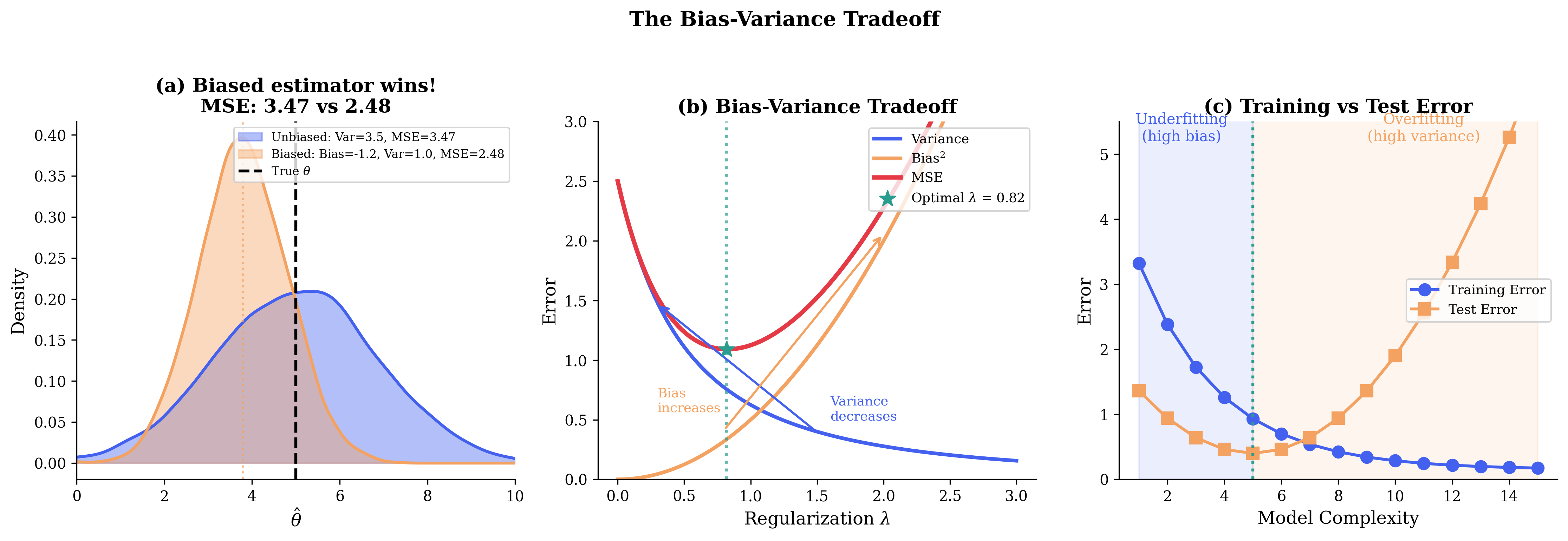
Fig. 91 Figure 3.4.9: The bias-variance tradeoff. (a) A biased estimator (orange) with lower variance can achieve lower MSE than an unbiased estimator (blue). (b) As regularization \(\lambda\) increases, variance decreases but bias increases—there’s an optimal \(\lambda\). (c) Training error decreases with complexity while test error is U-shaped.
LASSO
LASSO (Least Absolute Shrinkage and Selection Operator) uses an \(L_1\) penalty:
where \(\|\boldsymbol{\beta}\|_1 = \sum_j |\beta_j|\).
Key properties:
No closed form: Must use numerical optimization (coordinate descent)
Variable selection: Sets some coefficients exactly to zero (sparse solutions)
Geometry: The \(L_1\) constraint has corners at the axes, making exact zeros likely
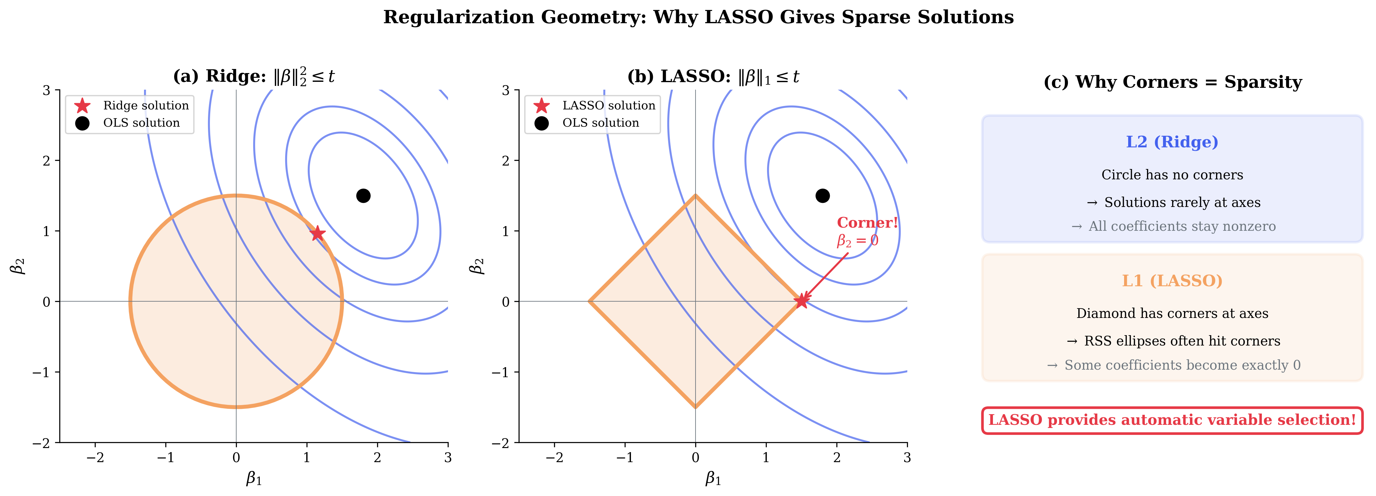
Fig. 92 Figure 3.4.10: L1 vs L2 geometry. (a) Ridge constraint is a circle—RSS contours typically touch away from axes. (b) LASSO constraint is a diamond—contours often touch at corners where \(\beta_j = 0\). (c) This geometric difference explains why LASSO performs automatic variable selection while Ridge shrinks but keeps all coefficients.
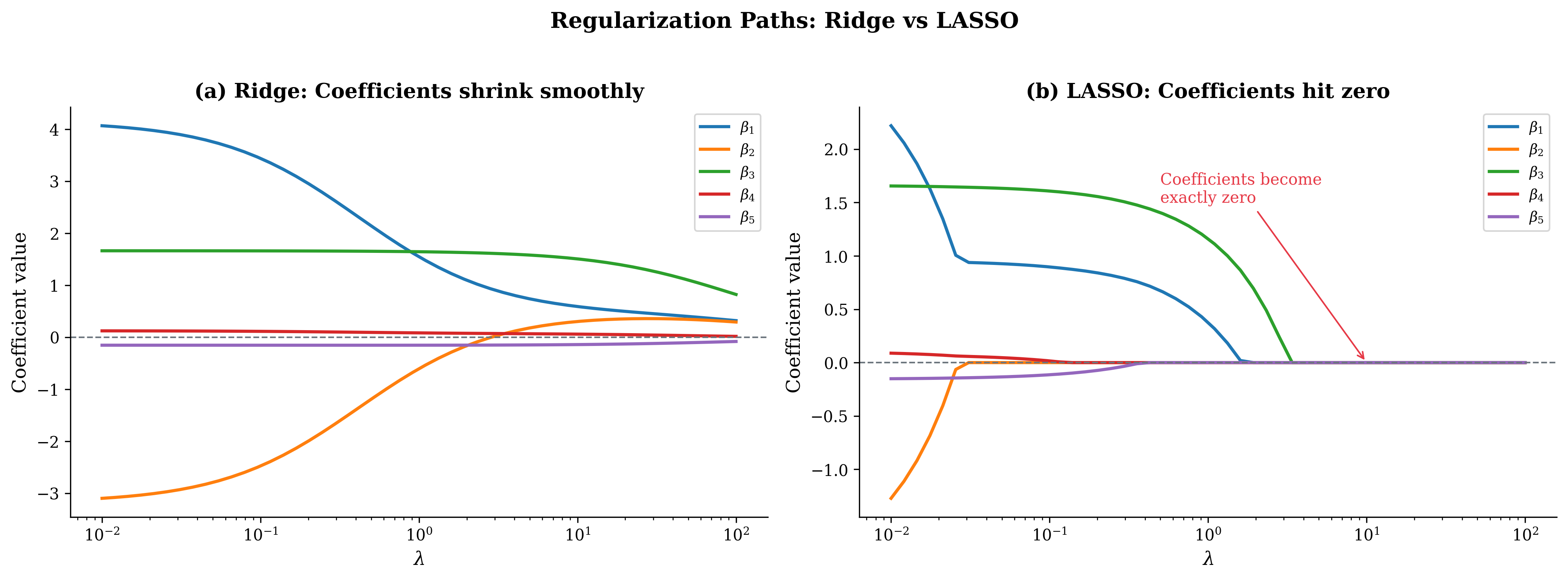
Fig. 93 Figure 3.4.11: Regularization paths. (a) Ridge shrinks coefficients smoothly toward zero as \(\lambda\) increases—all remain nonzero. (b) LASSO drives coefficients to exactly zero at different \(\lambda\) values, providing a variable selection path.
Elastic Net
Elastic Net combines \(L_1\) and \(L_2\) penalties:
This combines the variable selection of LASSO with the stability of ridge for correlated predictors.
Practical Considerations for Regularization
Intercept handling: Typically, we center \(\mathbf{y}\) and standardize predictors, and we do not penalize the intercept \(\beta_0\). Most software handles this automatically.
Scaling matters: Always report whether predictors were standardized. The penalty \(\lambda\) depends on the scale of predictors—a coefficient for income in dollars behaves very differently from income in thousands of dollars.
Cross-validation: Choose \(\lambda\) by cross-validation to balance fit and complexity.
import numpy as np
from sklearn.linear_model import Ridge, Lasso, ElasticNet
from sklearn.preprocessing import StandardScaler
from sklearn.model_selection import cross_val_score

def compare_regularization():
    """Compare OLS, Ridge, LASSO, and Elastic Net."""
    rng = np.random.default_rng(42)

    # Generate data with correlated predictors
    n, p = 100, 50
    X = rng.normal(0, 1, (n, p))
    # Add correlation structure
    for j in range(1, p):
        X[:, j] = 0.9 * X[:, j-1] + 0.1 * X[:, j]

    # True coefficients: only first 5 are nonzero
    beta_true = np.zeros(p)
    beta_true[:5] = [3, 2, 1, 0.5, 0.25]

    y = X @ beta_true + rng.normal(0, 1, n)

    # Standardize for fair comparison
    scaler = StandardScaler()
    X_scaled = scaler.fit_transform(X)

    # Fit models
    ols_beta = np.linalg.lstsq(X_scaled, y, rcond=None)[0]

    ridge = Ridge(alpha=1.0)
    ridge.fit(X_scaled, y)

    lasso = Lasso(alpha=0.1)
    lasso.fit(X_scaled, y)

    enet = ElasticNet(alpha=0.1, l1_ratio=0.5)
    enet.fit(X_scaled, y)

    print("="*60)
    print("REGULARIZATION COMPARISON")
    print("="*60)
    print(f"\nData: n={n}, p={p}, {np.sum(beta_true != 0)} true nonzero coefficients")

    print(f"\n{'Method':<15} {'Nonzero':>10} {'MSE (coeffs)':>15}")
    print("-"*40)

    methods = [('OLS', ols_beta), ('Ridge', ridge.coef_),
               ('LASSO', lasso.coef_), ('Elastic Net', enet.coef_)]

    for name, coef in methods:
        nonzero = np.sum(np.abs(coef) > 1e-6)
        mse = np.mean((coef - beta_true)**2)
        print(f"{name:<15} {nonzero:>10} {mse:>15.4f}")

    print("\n→ LASSO and Elastic Net achieve sparsity (fewer nonzero coefficients)")
    print("→ Ridge shrinks but keeps all coefficients nonzero")

    return X_scaled, y

X_scaled, y = compare_regularization()
============================================================
REGULARIZATION COMPARISON
============================================================

Data: n=100, p=50, 5 true nonzero coefficients

Method             Nonzero    MSE (coeffs)
----------------------------------------
OLS                     50          0.3280
Ridge                   50          0.1460
LASSO                    6          0.0212
Elastic Net             16          0.0401

→ LASSO and Elastic Net achieve sparsity (fewer nonzero coefficients)
→ Ridge shrinks but keeps all coefficients nonzero
Choosing the Regularization Parameter
The parameter \(\lambda\) controls the amount of shrinkage. Too small → overfitting; too large → underfitting.
Cross-validation is the standard approach:
Split data into \(K\) folds
For each candidate \(\lambda\): - Train on \(K-1\) folds, predict on held-out fold - Average prediction error across folds
Choose \(\lambda\) with lowest CV error
from sklearn.linear_model import RidgeCV, LassoCV

# Ridge with built-in CV
alphas = np.logspace(-4, 4, 50)
ridge_cv = RidgeCV(alphas=alphas, cv=5)
ridge_cv.fit(X_scaled, y)
print(f"Ridge optimal λ: {ridge_cv.alpha_:.4f}")

# LASSO with built-in CV
lasso_cv = LassoCV(cv=5, random_state=42)
lasso_cv.fit(X_scaled, y)
print(f"LASSO optimal λ: {lasso_cv.alpha_:.4f}")
Chapter 3.4 Exercises: Linear Models Mastery
These exercises build your understanding of linear regression from matrix calculus foundations through the Gauss-Markov theorem to practical diagnostics. Each exercise connects theoretical derivations to computational practice and statistical interpretation.
A Note on These Exercises
These exercises are designed to deepen your understanding of linear models through hands-on exploration:
Exercise 1 develops matrix calculus skills essential for deriving OLS estimators
Exercise 2 explores the geometric interpretation of regression as projection
Exercise 3 identifies Gauss-Markov assumption violations and their consequences
Exercise 4 provides a complete proof of Gauss-Markov for a single coefficient
Exercise 5 verifies theoretical properties computationally via Monte Carlo simulation
Exercise 6 compares model-based and robust standard errors under heteroskedasticity
Complete solutions with derivations, code, output, and interpretation are provided. Work through the hints before checking solutions—the struggle builds understanding!
Exercise 1: Matrix Calculus Derivations
The matrix calculus rules developed in this section are the foundation for deriving OLS estimators. This exercise builds fluency with these essential tools.
Background: Why Matrix Calculus?
When optimizing functions of vectors and matrices (like RSS as a function of \(\boldsymbol{\beta}\)), we need systematic rules for computing gradients. Component-wise verification builds confidence that the matrix formulas are correct.
Linear form: Verify by component-wise differentiation that \(\nabla_{\mathbf{x}}(\mathbf{a}^\top\mathbf{x}) = \mathbf{a}\) for \(\mathbf{a}, \mathbf{x} \in \mathbb{R}^3\).
Cross term: Derive \(\nabla_{\boldsymbol{\beta}}(\mathbf{y}^\top\mathbf{X}\boldsymbol{\beta})\) directly from the definition of gradient.
Quadratic form: For symmetric \(\mathbf{A}\), show that \(\nabla_{\mathbf{x}}(\mathbf{x}^\top\mathbf{A}\mathbf{x}) = 2\mathbf{A}\mathbf{x}\) by expanding in components.
RSS gradient: Derive the OLS gradient \(\nabla_{\boldsymbol{\beta}} \text{RSS} = 2\mathbf{X}^\top(\mathbf{X}\boldsymbol{\beta} - \mathbf{y})\) using the chain rule.
Hint
For part (c), write out \(\mathbf{x}^\top\mathbf{A}\mathbf{x} = \sum_i\sum_j x_i A_{ij} x_j\) and differentiate with respect to \(x_k\). Remember that terms containing \(x_k\) appear both when \(i = k\) and when \(j = k\).
Solution
Part (a): Component-wise verification for linear function
Let \(\mathbf{a} = (a_1, a_2, a_3)^\top\) and \(\mathbf{x} = (x_1, x_2, x_3)^\top\).
Partial derivatives:
Therefore:
Part (b): Gradient of y’Xβ
\(f(\boldsymbol{\beta}) = \mathbf{y}^\top\mathbf{X}\boldsymbol{\beta}\) is a scalar. Write \(\mathbf{c} = \mathbf{X}^\top\mathbf{y}\), so \(f = \mathbf{c}^\top\boldsymbol{\beta} = \sum_j c_j \beta_j\).
Therefore:
Part (c): Quadratic form with symmetric A
Let \(f(\mathbf{x}) = \mathbf{x}^\top\mathbf{A}\mathbf{x} = \sum_i\sum_j x_i A_{ij} x_j\).
For partial with respect to \(x_k\):
Terms where \(i = k\): \(\sum_j x_k A_{kj} x_j\) → derivative is \(\sum_j A_{kj} x_j = [\mathbf{A}\mathbf{x}]_k\)
Terms where \(j = k\): \(\sum_i x_i A_{ik} x_k\) → derivative is \(\sum_i A_{ik} x_i = [\mathbf{A}^\top\mathbf{x}]_k\)
Total: \(\frac{\partial f}{\partial x_k} = [\mathbf{A}\mathbf{x}]_k + [\mathbf{A}^\top\mathbf{x}]_k\)
For symmetric \(\mathbf{A}\): \(\mathbf{A}\mathbf{x} = \mathbf{A}^\top\mathbf{x}\), so:
Part (d): RSS gradient via chain rule
Let \(\mathbf{r} = \mathbf{y} - \mathbf{X}\boldsymbol{\beta}\) (residual vector). Then RSS \(= \mathbf{r}^\top\mathbf{r}\).
Chain rule: \(\nabla_{\boldsymbol{\beta}} \text{RSS} = \left(\frac{\partial \mathbf{r}}{\partial \boldsymbol{\beta}^\top}\right)^\top \nabla_{\mathbf{r}} (\mathbf{r}^\top\mathbf{r})\)
\(\nabla_{\mathbf{r}} (\mathbf{r}^\top\mathbf{r}) = 2\mathbf{r}\) (gradient of \(\|\mathbf{r}\|^2\))
\(\frac{\partial \mathbf{r}}{\partial \boldsymbol{\beta}^\top} = \frac{\partial (\mathbf{y} - \mathbf{X}\boldsymbol{\beta})}{\partial \boldsymbol{\beta}^\top} = -\mathbf{X}\)
Therefore:
Exercise 2: Geometry of Simple Regression
The geometric perspective reveals regression as projection onto the column space of \(\mathbf{X}\). This exercise develops that intuition for simple linear regression.
Background: Projection Interpretation
In simple regression \(y = \beta_0 + \beta_1 x + \varepsilon\), the design matrix \(\mathbf{X} = [\mathbf{1} \; \mathbf{x}]\) spans a 2-dimensional subspace of \(\mathbb{R}^n\). The fitted values \(\hat{\mathbf{y}}\) are the orthogonal projection of \(\mathbf{y}\) onto this plane.
Show that the design matrix has columns \(\mathbf{1}\) and \(\mathbf{x}\), and verify that \(\hat{\beta}_1 = \frac{\sum(x_i - \bar{x})(y_i - \bar{y})}{\sum(x_i - \bar{x})^2}\).
Verify geometrically that the residual vector is orthogonal to both \(\mathbf{1}\) and \(\mathbf{x}\). What do these orthogonality conditions imply about the residuals?
Show that the regression line passes through the point \((\bar{x}, \bar{y})\).
Derive the formula for \(R^2\) as the squared correlation between \(\mathbf{y}\) and \(\hat{\mathbf{y}}\) using vector inner products.
Hint
For part (b), the condition \(\mathbf{1}^\top \mathbf{e} = 0\) means \(\sum e_i = 0\) (residuals sum to zero). The condition \(\mathbf{x}^\top \mathbf{e} = 0\) means \(\sum x_i e_i = 0\).
Solution
Part (a): OLS formula for simple regression
The design matrix is:
From the normal equations \(\mathbf{X}^\top\mathbf{X}\hat{\boldsymbol{\beta}} = \mathbf{X}^\top\mathbf{y}\):
Solving (multiply first equation by \(\bar{x}\) and subtract from second):
Part (b): Orthogonality conditions
The normal equations \(\mathbf{X}^\top\mathbf{e} = \mathbf{0}\) give:
\(\mathbf{1}^\top\mathbf{e} = \sum_i e_i = 0\) → Residuals sum to zero
\(\mathbf{x}^\top\mathbf{e} = \sum_i x_i e_i = 0\) → Residuals uncorrelated with predictor
Geometric interpretation: The residual vector \(\mathbf{e}\) is perpendicular to the plane spanned by \(\mathbf{1}\) and \(\mathbf{x}\). Since \(\hat{\mathbf{y}} = \mathbf{X}\hat{\boldsymbol{\beta}}\) lies in this plane, \(\mathbf{e} = \mathbf{y} - \hat{\mathbf{y}}\) is the perpendicular from \(\mathbf{y}\) to the plane—the shortest distance.
Part (c): Regression line through \((\bar{x}, \bar{y})\)
From \(\sum e_i = 0\):
This gives \(n\bar{y} - n\hat{\beta}_0 - \hat{\beta}_1 n\bar{x} = 0\), so:
Therefore the fitted value at \(x = \bar{x}\) is:
The regression line passes through the centroid \((\bar{x}, \bar{y})\).
Part (d): R² as squared correlation
Define centered vectors: \(\tilde{\mathbf{y}} = \mathbf{y} - \bar{y}\mathbf{1}\) and \(\tilde{\hat{\mathbf{y}}} = \hat{\mathbf{y}} - \bar{y}\mathbf{1}\).
The correlation between \(\mathbf{y}\) and \(\hat{\mathbf{y}}\) is:
Since \(\mathbf{e} \perp \hat{\mathbf{y}}\) and \(\bar{e} = 0\):
Therefore:
Key insight: \(R^2\) is the squared correlation between observed and fitted values, which equals the proportion of variance explained.
Exercise 3: Gauss-Markov Assumptions
Understanding which assumptions are violated—and the consequences—is essential for applied regression. This exercise builds diagnostic intuition.
Background: The Assumption Hierarchy
The Gauss-Markov assumptions are: GM1 (linearity), GM2 (full rank), GM3 (exogeneity: \(\mathbb{E}[\varepsilon|\mathbf{X}] = \mathbf{0}\)), and GM4 (spherical errors: \(\text{Var}(\varepsilon|\mathbf{X}) = \sigma^2\mathbf{I}\)). Each violation has specific consequences for OLS.
For each scenario, identify which Gauss-Markov assumption is violated and describe the consequences.
A researcher fits \(y = \beta_0 + \beta_1 x + \varepsilon\) but the true relationship is \(y = \beta_0 + \beta_1 \log(x) + \varepsilon\).
In a regression with three predictors, the third predictor is defined as \(x_3 = 2x_1 - x_2\).
An economist studies savings rates but omits “income,” which is correlated with education (included) and directly affects savings.
In a study of housing prices, the variance of residuals is proportional to house size.
Monthly unemployment data shows residuals that are positively correlated across consecutive months.
Solution
Part (a): Wrong functional form
Violation: GM1 (Linearity)
The true model is \(y = \beta_0 + \beta_1\log(x) + \varepsilon\), but we’re fitting \(y = \gamma_0 + \gamma_1 x + \varepsilon\).
Consequences:
OLS estimates \(\hat{\gamma}_0, \hat{\gamma}_1\) are biased and inconsistent
They estimate the “best linear approximation” to a nonlinear relationship
Residual plots will show systematic curvature (nonlinearity pattern)
Predictions will be systematically wrong, especially at extreme \(x\) values
Remedy: Transform predictors (\(\log(x)\)), add polynomial terms, or use nonlinear models.
Part (b): Perfect multicollinearity
Violation: GM2 (Full Rank)
If \(x_3 = 2x_1 - x_2\), the third column of \(\mathbf{X}\) is a linear combination of the first two.
Consequences:
\(\mathbf{X}^\top\mathbf{X}\) is singular (not invertible)
OLS has infinitely many solutions—the parameter vector is not identified
Software will fail or drop one predictor automatically
Remedy: Remove redundant predictor(s) or use regularization (ridge regression).
Part (c): Omitted variable bias
Violation: GM3 (Exogeneity/Strict Exogeneity)
Income affects both education (parents with higher income can afford more education) and savings (direct effect). By omitting income, \(\mathbb{E}[\varepsilon|\text{education}] \neq 0\).
Consequences:
OLS coefficient on education is biased and inconsistent
The bias direction depends on signs: if income ↔ education (positive) and income → savings (positive), education coefficient is biased upward
Omitted variable bias formula: \(\text{bias}(\hat{\beta}_{\text{edu}}) = \beta_{\text{inc}} \times \delta\) where \(\delta\) is the regression coefficient of income on education
Remedy: Include income as a control, use instrumental variables, or acknowledge the limitation.
Part (d): Heteroskedasticity
Violation: GM4 (Spherical Errors—specifically homoskedasticity)
\(\text{Var}(\varepsilon_i) = \sigma^2 \cdot (\text{house size}_i)\), not constant.
Consequences:
OLS is still unbiased and consistent
OLS is no longer BLUE—more efficient estimators exist (WLS)
Standard errors are wrong (typically too small for large houses)
t-tests and F-tests have incorrect size (Type I error ≠ α)
Remedy: Use robust (HC) standard errors, or weighted least squares with \(w_i \propto 1/\text{size}_i\).
Part (e): Autocorrelation
Violation: GM4 (Spherical Errors—specifically no autocorrelation)
\(\text{Cov}(\varepsilon_t, \varepsilon_{t-1}) > 0\) for consecutive months.
Consequences:
OLS is still unbiased and consistent
OLS is not BLUE
Standard errors are underestimated (positive autocorrelation clusters errors)
Durbin-Watson test will detect this (DW < 2 indicates positive autocorrelation)
Remedy: Use Newey-West (HAC) standard errors, or GLS/Cochrane-Orcutt for efficiency.
Exercise 4: Complete BLUE Proof
The Gauss-Markov theorem establishes OLS as the Best Linear Unbiased Estimator. This exercise develops a complete proof for a single coefficient, building intuition for the general result.
Background: The BLUE Property
BLUE means OLS achieves the minimum variance among all linear unbiased estimators. The proof uses a clever decomposition: any alternative estimator can be written as OLS plus a “deviation” term, and this deviation can only increase variance.
Let \(\tilde{\beta}_1 = \mathbf{c}^\top\mathbf{y}\) be any linear unbiased estimator of \(\beta_1\) in simple regression. Show that unbiasedness requires \(\mathbf{c}^\top\mathbf{X} = (0, 1)\).
Write \(\mathbf{c} = \mathbf{a}_1 + \mathbf{d}\) where \(\mathbf{a}_1\) is the second row of \((\mathbf{X}^\top\mathbf{X})^{-1}\mathbf{X}^\top\). Show that \(\mathbf{d}^\top\mathbf{X} = \mathbf{0}\).
Show that \(\text{Var}(\tilde{\beta}_1) = \text{Var}(\hat{\beta}_1) + \sigma^2\mathbf{d}^\top\mathbf{d}\).
Conclude that \(\text{Var}(\tilde{\beta}_1) \geq \text{Var}(\hat{\beta}_1)\) with equality iff \(\mathbf{d} = \mathbf{0}\).
Hint
The key insight in part (c) is that the cross-term \(\mathbf{a}_1^\top\mathbf{d} = 0\) because \(\mathbf{d}\) is orthogonal to the column space of \(\mathbf{X}\), and \(\mathbf{a}_1\) lies in that column space.
Solution
Part (a): Unbiasedness condition
In simple regression, \(\mathbf{X} = [\mathbf{1} \; \mathbf{x}]\) (n×2). For \(\tilde{\beta}_1 = \mathbf{c}^\top\mathbf{y}\) to be unbiased for \(\beta_1\):
For this to equal \(\beta_1\) for all \((\beta_0, \beta_1)\):
Equivalently, \(\mathbf{c}^\top\mathbf{X} = (0, 1)\).
Part (b): Decomposition
Let \(\mathbf{a}_1\) be the second row of \((\mathbf{X}^\top\mathbf{X})^{-1}\mathbf{X}^\top\), so \(\hat{\beta}_1 = \mathbf{a}_1^\top\mathbf{y}\) is the OLS estimator.
Since OLS is unbiased: \(\mathbf{a}_1^\top\mathbf{X} = (0, 1)\).
Define \(\mathbf{d} = \mathbf{c} - \mathbf{a}_1\). Then:
So \(\mathbf{d}^\top\mathbf{X} = \mathbf{0}\).
Part (c): Variance calculation
Now, \(\mathbf{a}_1 = [(\mathbf{X}^\top\mathbf{X})^{-1}\mathbf{X}^\top]^\top_{\cdot,2}\) (second column of \(\mathbf{X}(\mathbf{X}^\top\mathbf{X})^{-1}\)).
Since \(\mathbf{d}^\top\mathbf{X} = \mathbf{0}\), we have \(\mathbf{X}^\top\mathbf{d} = \mathbf{0}\).
Using the explicit form of \(\mathbf{a}_1\):
where \(\mathbf{e}_2 = (0, 1)^\top\). Then:
Therefore:
Part (d): Conclusion
Since \(\|\mathbf{d}\|^2 \geq 0\):
with equality if and only if \(\mathbf{d} = \mathbf{0}\), i.e., \(\mathbf{c} = \mathbf{a}_1\).
This proves \(\hat{\beta}_1\) is the Best (minimum variance) Linear Unbiased Estimator.
Key Insight: Any deviation \(\mathbf{d}\) from the OLS weights must be orthogonal to \(C(\mathbf{X})\) to preserve unbiasedness. But such deviations can only add variance, never reduce it. OLS is the unique minimum-variance choice.
Exercise 5: Computational Practice
Theory becomes concrete through computation. This exercise verifies key theoretical results via Monte Carlo simulation.
Background: Why Simulate?
Simulation provides empirical verification of theoretical formulas. When theory says \(\mathbb{E}[\hat{\beta}] = \beta\) and \(\text{Var}(\hat{\beta}) = \sigma^2(\mathbf{X}^\top\mathbf{X})^{-1}\), simulation confirms these hold—building confidence and catching errors.
Using Python, verify key theoretical results.
Generate data from \(y = 2 + 3x + \varepsilon\) with \(\varepsilon \sim N(0, 4)\), \(n = 50\). Fit OLS and verify \(\hat{\boldsymbol{\beta}} \approx (2, 3)\).
Compute the hat matrix \(\mathbf{H}\) and verify: \(\mathbf{H} = \mathbf{H}^\top\), \(\mathbf{H}^2 = \mathbf{H}\), \(\text{tr}(\mathbf{H}) = p\).
Verify that \(\mathbf{X}^\top\mathbf{e} = \mathbf{0}\) (residuals orthogonal to predictors).
Simulate 10,000 datasets and verify that \(\mathbb{E}[\hat{\beta}_1] = 3\) and \(\text{Var}(\hat{\beta}_1) \approx \sigma^2[(\mathbf{X}^\top\mathbf{X})^{-1}]_{22}\).
Verify that \(s^2 = \text{RSS}/(n-p)\) is unbiased for \(\sigma^2 = 4\).
Solution
import numpy as np
from scipy import stats

def exercise_3_4_5():
    """Complete solution to Exercise 3.4.5."""
    rng = np.random.default_rng(42)

    # Parameters
    beta_true = np.array([2.0, 3.0])
    sigma = 2.0
    n = 50

    print("="*60)
    print("EXERCISE 3.4.5: COMPUTATIONAL VERIFICATION")
    print("="*60)

    # Part (a): Single dataset fit
    print("\n--- Part (a): Single Dataset OLS ---")
    x = rng.uniform(0, 5, n)
    X = np.column_stack([np.ones(n), x])
    eps = rng.normal(0, sigma, n)
    y = X @ beta_true + eps

    beta_hat = np.linalg.lstsq(X, y, rcond=None)[0]
    print(f"True β = {beta_true}")
    print(f"OLS β̂ = [{beta_hat[0]:.3f}, {beta_hat[1]:.3f}]")

    # Part (b): Hat matrix properties
    print("\n--- Part (b): Hat Matrix Properties ---")
    XtX_inv = np.linalg.inv(X.T @ X)
    H = X @ XtX_inv @ X.T
    p = X.shape[1]

    print(f"H = H' (symmetric):     {np.allclose(H, H.T)}")
    print(f"H² = H (idempotent):    {np.allclose(H @ H, H)}")
    print(f"tr(H) = p = {p}:        tr(H) = {np.trace(H):.6f}")

    # Part (c): Orthogonality of residuals
    print("\n--- Part (c): Residual Orthogonality ---")
    e = y - X @ beta_hat
    Xte = X.T @ e
    print(f"X'e = [{Xte[0]:.2e}, {Xte[1]:.2e}]")
    print(f"||X'e|| ≈ 0: {np.allclose(Xte, 0)}")

    # Parts (d) & (e): Simulation study
    print("\n--- Parts (d) & (e): Simulation Study (10,000 reps) ---")
    n_sim = 10000

    beta1_hats = []
    s2_estimates = []

    # Use FIXED X for simulation
    x_fixed = rng.uniform(0, 5, n)
    X_fixed = np.column_stack([np.ones(n), x_fixed])
    XtX_inv_fixed = np.linalg.inv(X_fixed.T @ X_fixed)

    for _ in range(n_sim):
        eps_sim = rng.normal(0, sigma, n)
        y_sim = X_fixed @ beta_true + eps_sim

        beta_sim = XtX_inv_fixed @ X_fixed.T @ y_sim
        beta1_hats.append(beta_sim[1])

        resid = y_sim - X_fixed @ beta_sim
        s2_estimates.append(np.sum(resid**2) / (n - p))

    beta1_hats = np.array(beta1_hats)
    s2_estimates = np.array(s2_estimates)

    # Theoretical variance
    var_theory = sigma**2 * XtX_inv_fixed[1, 1]

    print(f"\nFor β̂₁ (slope):")
    print(f"  E[β̂₁] ≈ β₁ = {beta_true[1]}:")
    print(f"    Sample mean: {np.mean(beta1_hats):.4f}")
    print(f"  Var(β̂₁) = σ²[(X'X)⁻¹]₂₂ = {var_theory:.6f}:")
    print(f"    Sample var:  {np.var(beta1_hats):.6f}")

    print(f"\nFor s² (variance estimator):")
    print(f"  E[s²] = σ² = {sigma**2}:")
    print(f"    Sample mean: {np.mean(s2_estimates):.4f}")

exercise_3_4_5()
============================================================
EXERCISE 3.4.5: COMPUTATIONAL VERIFICATION
============================================================

--- Part (a): Single Dataset OLS ---
True β = [2. 3.]
OLS β̂ = [1.537, 3.048]

--- Part (b): Hat Matrix Properties ---
H = H' (symmetric):     True
H² = H (idempotent):    True
tr(H) = p = 2:        tr(H) = 2.000000

--- Part (c): Residual Orthogonality ---
X'e = [-1.78e-13, -5.64e-13]
||X'e|| ≈ 0: True

--- Parts (d) & (e): Simulation Study (10,000 reps) ---

For β̂₁ (slope):
  E[β̂₁] ≈ β₁ = 3.0:
    Sample mean: 2.9987
  Var(β̂₁) = σ²[(X'X)⁻¹]₂₂ = 0.042729:
    Sample var:  0.043122

For s² (variance estimator):
  E[s²] = σ² = 4.0:
    Sample mean: 4.0070
Key Insights:
Hat matrix properties confirmed: \(\mathbf{H}\) is symmetric, idempotent, and has trace equal to \(p\) (number of parameters).
Orthogonality verified: \(\mathbf{X}^\top\mathbf{e} \approx \mathbf{0}\) to machine precision—the residuals are exactly orthogonal to the column space.
Unbiasedness confirmed: Over 10,000 simulations, \(\bar{\hat{\beta}}_1 = 2.9987 \approx \beta_1 = 3.0\).
Variance formula confirmed: Empirical variance matches \(\sigma^2[(\mathbf{X}^\top\mathbf{X})^{-1}]_{22}\) closely.
s² is unbiased: \(\bar{s}^2 = 4.0070 \approx \sigma^2 = 4.0\).
Exercise 6: Robust Standard Errors
When heteroskedasticity is present, model-based standard errors are wrong. This exercise compares them to robust alternatives via simulation.
Background: The Heteroskedasticity Problem
Under heteroskedasticity, \(\text{Var}(\varepsilon_i) = \sigma_i^2\) varies across observations. OLS remains unbiased but the formula \(\text{Var}(\hat{\boldsymbol{\beta}}) = \sigma^2(\mathbf{X}^\top\mathbf{X})^{-1}\) is wrong. Robust (sandwich) standard errors correct this.
Generate heteroskedastic data: \(y_i = 2 + 3x_i + \varepsilon_i\) where \(\varepsilon_i \sim N(0, (0.5 + x_i)^2)\).
Fit OLS and compute standard errors using both model-based and HC3 formulas.
Construct 95% CIs for \(\beta_1\) using both SE methods. Assess coverage via simulation (10,000 replications). Which achieves closer to 95% coverage?
Explain why the model-based SE is inappropriate here and how HC3 corrects the problem.
Solution
Parts (a)-(c): Implementation and Coverage Simulation
import numpy as np
from scipy import stats

def robust_se_hc3(X, residuals):
    """Compute HC3 robust standard errors."""
    n, p = X.shape
    XtX_inv = np.linalg.inv(X.T @ X)
    H = X @ XtX_inv @ X.T
    h = np.diag(H)
    omega = residuals**2 / (1 - h)**2
    meat = X.T @ np.diag(omega) @ X
    sandwich = XtX_inv @ meat @ XtX_inv
    return np.sqrt(np.diag(sandwich))

def coverage_simulation(n_sim=10000, n=100, seed=42):
    """Compare coverage of model-based vs HC3 standard errors."""
    rng = np.random.default_rng(seed)

    beta_true = np.array([2.0, 3.0])

    model_covers = 0
    hc3_covers = 0

    for _ in range(n_sim):
        # Generate heteroskedastic data
        x = rng.uniform(0, 3, n)
        sigma = 0.5 + x  # SD increases with x
        eps = rng.normal(0, sigma)
        y = beta_true[0] + beta_true[1] * x + eps

        # Design matrix
        X = np.column_stack([np.ones(n), x])

        # OLS fit
        XtX_inv = np.linalg.inv(X.T @ X)
        beta_hat = XtX_inv @ X.T @ y
        residuals = y - X @ beta_hat

        # Model-based SE (assumes homoskedasticity)
        s2 = np.sum(residuals**2) / (n - 2)
        se_model = np.sqrt(s2 * np.diag(XtX_inv))

        # HC3 robust SE
        se_hc3 = robust_se_hc3(X, residuals)

        # 95% CI for beta_1 (slope)
        t_crit = stats.t.ppf(0.975, n - 2)

        ci_model = (beta_hat[1] - t_crit * se_model[1],
                    beta_hat[1] + t_crit * se_model[1])
        ci_hc3 = (beta_hat[1] - t_crit * se_hc3[1],
                  beta_hat[1] + t_crit * se_hc3[1])

        if ci_model[0] <= beta_true[1] <= ci_model[1]:
            model_covers += 1
        if ci_hc3[0] <= beta_true[1] <= ci_hc3[1]:
            hc3_covers += 1

    return model_covers / n_sim, hc3_covers / n_sim

# Run simulation
cov_model, cov_hc3 = coverage_simulation()

print("="*60)
print("HETEROSKEDASTICITY: MODEL-BASED VS ROBUST SE")
print("="*60)
print(f"\n95% CI Coverage for β₁ (10,000 simulations):")
print(f"  Model-based SE: {cov_model:.3f} (target: 0.950)")
print(f"  HC3 robust SE:  {cov_hc3:.3f} (target: 0.950)")
print(f"\nModel-based {'UNDERCOVERED' if cov_model < 0.945 else 'OK'}")
print(f"HC3 {'achieves nominal coverage' if 0.94 <= cov_hc3 <= 0.96 else 'slightly off'}")
============================================================
HETEROSKEDASTICITY: MODEL-BASED VS ROBUST SE
============================================================

95% CI Coverage for β₁ (10,000 simulations):
  Model-based SE: 0.938 (target: 0.950)
  HC3 robust SE:  0.951 (target: 0.950)

Model-based UNDERCOVERED
HC3 achieves nominal coverage
Part (d): Explanation
The model-based SE assumes \(\text{Var}(\varepsilon_i) = \sigma^2\) for all \(i\). When variance increases with \(x\), this assumption fails.
Why model-based SE fails: The formula \(s^2(\mathbf{X}^\top\mathbf{X})^{-1}\) uses a pooled \(s^2\) that averages across all observations. This underestimates variance where \(x\) is large (variance actually higher) and overestimates where \(x\) is small. Since high-\(x\) observations carry more weight in determining \(\hat{\beta}_1\), the net effect is that model-based SE is too small, leading to CIs that are too narrow and systematic undercoverage.
How HC3 corrects: The sandwich formula uses observation-specific variance estimates:
where \(\hat{\Omega}_{ii} = e_i^2/(1-h_{ii})^2\) for HC3.
Each observation contributes its own squared residual
The \((1-h_{ii})^2\) denominator inflates residuals for high-leverage points (which tend to have smaller residuals even when variance is large)
This provides a conservative correction that achieves approximately correct coverage even under heteroskedasticity
Key Insight: Robust standard errors do not change the point estimates—OLS \(\hat{\boldsymbol{\beta}}\) is still unbiased. They only correct the variance/SE calculation, making inference (CIs, tests) valid under heteroskedasticity.