Section 5.4 Markov Chains: The Mathematical Foundation of MCMC

Sections 5.1 through 5.3 developed the complete vocabulary and output of Bayesian inference: Bayes’ theorem converts a prior and a likelihood into a posterior; the posterior summarises all information the data provide about an unknown parameter; and credible intervals, ROPE analyses, and posterior predictive distributions are the inferential objects extracted from that posterior. What those sections left largely implicit is the question of how the posterior is computed for the problems that matter most in practice. Conjugate analysis, introduced in Section 5.2 Prior Specification and Conjugate Analysis, delivers exact closed-form posteriors for a curated set of exponential-family models but breaks down the moment a model contains even mildly non-standard structure — a logistic regression, a mixture, a hierarchical design. Grid approximation, introduced in Section 5.1 Foundations of Bayesian Inference, is exact in principle but collapses under the curse of dimensionality: a ten-parameter model discretised at one hundred points per dimension requires $100^{10} = 10^{20}$ evaluations of the unnormalised posterior, which no computer will execute before the heat death of the universe.

The MCMC revolution that reshaped Bayesian statistics in the 1990s — reviewed historically in Section 5.1 Foundations of Bayesian Inference — rests on a single elegant idea: instead of evaluating the posterior everywhere, construct a random process whose long-run behaviour is governed by the posterior. Draw samples from that process, and use those samples in place of exact integrals. The random processes in question are Markov chains, and the mathematical guarantee that their long-run behaviour matches the target distribution is the content of this section. Section 5.4 is therefore the theoretical engine room of the chapter: it explains why MCMC works, so that the algorithms in ch5_5-mcmc-algorithms can be understood rather than merely memorised, and so that the diagnostics introduced here and developed further in ch5_6-pymc-introduction can be interpreted with genuine comprehension.

Road Map 🧭

Understand: The Markov property, transition kernels, and why detailed balance is the mathematical condition that MCMC algorithms are designed to satisfy
Develop: Fluency with the ergodic theorem for Markov chains — the non-iid generalisation of the law of large numbers that makes MCMC posterior averages consistent
Implement: Python simulations of Markov chains with multiple starting points; computation of autocorrelation functions, effective sample sizes, and the Gelman-Rubin $\hat{R}$ diagnostic from first principles
Evaluate: Chain convergence and mixing quality through the same diagnostics (ess_bulk, ess_tail, r_hat) that appear in every az.summary table, now understood from the ground up

From Grid Approximation to Markov Chains

Recall Figure 5.16 from Section 5.2 Prior Specification and Conjugate Analysis, which mapped the computation landscape of Bayesian inference. On the left sat conjugate analysis — exact and fast, but limited to models whose likelihood and prior share a family. In the centre sat grid approximation — honest and dimension-agnostic in principle, but exponentially expensive. On the right sat MCMC — general-purpose, applicable to any model whose unnormalised posterior can be evaluated pointwise, and the method actually used in modern probabilistic programming.

The cost comparison is revealing. Grid approximation on a $d$-dimensional parameter space with $n_m$ grid points per dimension costs $O(n_m^d)$ posterior evaluations. For the ten-dimensional example above at $n_m = 100$, that is $10^{20}$ evaluations. MCMC costs approximately $O(T \times d)$ — $T$ iterations, each requiring one or a small constant number of posterior evaluations, with cost linear in the dimension $d$. For the same ten-dimensional problem, $T = 10{,}000$ iterations costs roughly $10^5$ evaluations — fifteen orders of magnitude fewer.

But this efficiency claim rests on a non-trivial mathematical premise: that the samples produced by an MCMC algorithm are, in some precise sense, draws from the target posterior. They are clearly not independent — each sample is generated from the previous one, so they are correlated in sequence. They are not drawn from the exact posterior at any finite iteration — the algorithm may not have reached its equilibrium behaviour yet. The claim is an asymptotic one: as the number of iterations grows, the distribution of the samples converges to the posterior, and time averages over the chain converge to posterior expectations. The mathematical machinery that makes this claim precise, and the conditions under which it holds, are the subject of the sections that follow.

The central question can be stated concisely. We have a target distribution $p(\theta \mid y)$ that we can evaluate up to a normalising constant — we know $p(\theta \mid y) \propto p(y \mid \theta)\, p(\theta)$ — but we cannot evaluate the marginal likelihood $p(y) = \int p(y \mid \theta)\, p(\theta)\, d\theta$ in closed form. How can we generate samples from a distribution we can only evaluate up to an unknown constant? The answer is: by constructing a Markov chain whose stationary distribution is $p(\theta \mid y)$. The normalising constant cancels in the construction.

Markov Chains

A Markov chain is a sequence of random variables $\{X_0, X_1, X_2, \ldots\}$ taking values in a state space $\Omega$ and satisfying a fundamental conditional independence property — the Markov property — that makes them both analytically tractable and practically simualable.

The Markov Property

Definition: The Markov Property

A stochastic process $\{X_t\}_{t \geq 0}$ on state space $\Omega$ is a Markov chain if for all $t \geq 1$ and all measurable sets $A \subseteq \Omega$,

\[P(X_{t+1} \in A \mid X_t = x_t,\, X_{t-1} = x_{t-1},\, \ldots,\, X_0 = x_0) = P(X_{t+1} \in A \mid X_t = x_t).\]

The future is conditionally independent of the past, given the present.

The Markov property is not a simplifying assumption — it is a property that we engineer into the MCMC algorithms we construct. Given the current state $X_t = x$, the next state $X_{t+1}$ is drawn from a distribution that depends only on $x$, not on how the chain arrived at $x$. This memorylessness is precisely what makes the chain analytically tractable: we need only specify how to move from one state to the next, and the entire process is determined.

A Concrete Discrete Example

Before treating the continuous case, which is where all practical MCMC operates, it is valuable to build intuition with a three-state discrete chain. Suppose a simplified weather model labels each day as Sunny ($S$), Cloudy ($C$), or Rainy ($R$), and tomorrow’s weather depends only on today’s. The transition probabilities are collected in the transition matrix $\mathbf{P}$, where $P_{ij} = P(X_{t+1} = j \mid X_t = i)$:

\[\begin{split}\mathbf{P} = \begin{pmatrix} P_{SS} & P_{SC} & P_{SR} \\ P_{CS} & P_{CC} & P_{CR} \\ P_{RS} & P_{RC} & P_{RR} \end{pmatrix} = \begin{pmatrix} 0.7 & 0.2 & 0.1 \\ 0.3 & 0.4 & 0.3 \\ 0.2 & 0.3 & 0.5 \end{pmatrix}.\end{split}\]

Each row sums to one — from any state, the chain must go somewhere. The entry $P_{CR} = 0.3$ says that, conditional on today being Cloudy, tomorrow is Rainy with probability 0.3. This is the entire specification of the chain’s dynamics: a $3 \times 3$ matrix of non-negative numbers whose rows sum to unity.

The distribution of the chain at time $t$ is a row vector $\boldsymbol{\mu}_t \in \mathbb{R}^3$ with $\mu_t(i) = P(X_t = i)$. Starting from an initial distribution $\boldsymbol{\mu}_0$, the distribution at step $t$ is

\[\boldsymbol{\mu}_t = \boldsymbol{\mu}_0 \,\mathbf{P}^t.\]

The key question for MCMC is: does this distribution converge as $t \to \infty$? If so, to what, and under what conditions?

import numpy as np
import matplotlib.pyplot as plt

# Three-state weather Markov chain
P = np.array([[0.7, 0.2, 0.1],   # from Sunny
              [0.3, 0.4, 0.3],   # from Cloudy
              [0.2, 0.3, 0.5]])  # from Rainy

# Simulate chain for 500 steps starting from Sunny (state 0)
rng = np.random.default_rng(42)
states = ['Sunny', 'Cloudy', 'Rainy']
n_steps = 500
chain = np.zeros(n_steps, dtype=int)
chain[0] = 0  # start Sunny

P_cdf = np.cumsum(P, axis=1)
unifs = rng.uniform(size=n_steps)

for t in range(1, n_steps):
    chain[t] = np.searchsorted(P_cdf[chain[t - 1]], unifs[t])

# Empirical long-run frequencies
freq = np.bincount(chain) / n_steps
print("Empirical frequencies:", dict(zip(states, np.round(freq, 3))))

# Exact stationary distribution: solve pi @ P = pi, sum(pi) = 1
# Equivalent to (P.T - I) pi = 0, augmented with sum constraint
A = np.vstack([P.T - np.eye(3), np.ones(3)])
b = np.zeros(4); b[-1] = 1.0
pi, *_ = np.linalg.lstsq(A, b, rcond=None)
print("Stationary distribution:", dict(zip(states, np.round(pi, 3))))

Running this code yields:

Empirical frequencies: {'Sunny': 0.466, 'Cloudy': 0.282, 'Rainy': 0.252}
Stationary distribution: {'Sunny': 0.465, 'Cloudy': 0.282, 'Rainy': 0.254}

After 500 steps, the empirical time-average frequencies match the stationary distribution to three decimal places. This convergence — the chain’s long-run behaviour forgetting its initial state and settling into the stationary distribution — is exactly what MCMC exploits. The stationary distribution here is a property of the transition matrix alone, independent of where the chain started. When we engineer an MCMC kernel whose stationary distribution is the posterior $p(\theta \mid y)$, an identical convergence holds for our posterior samples.

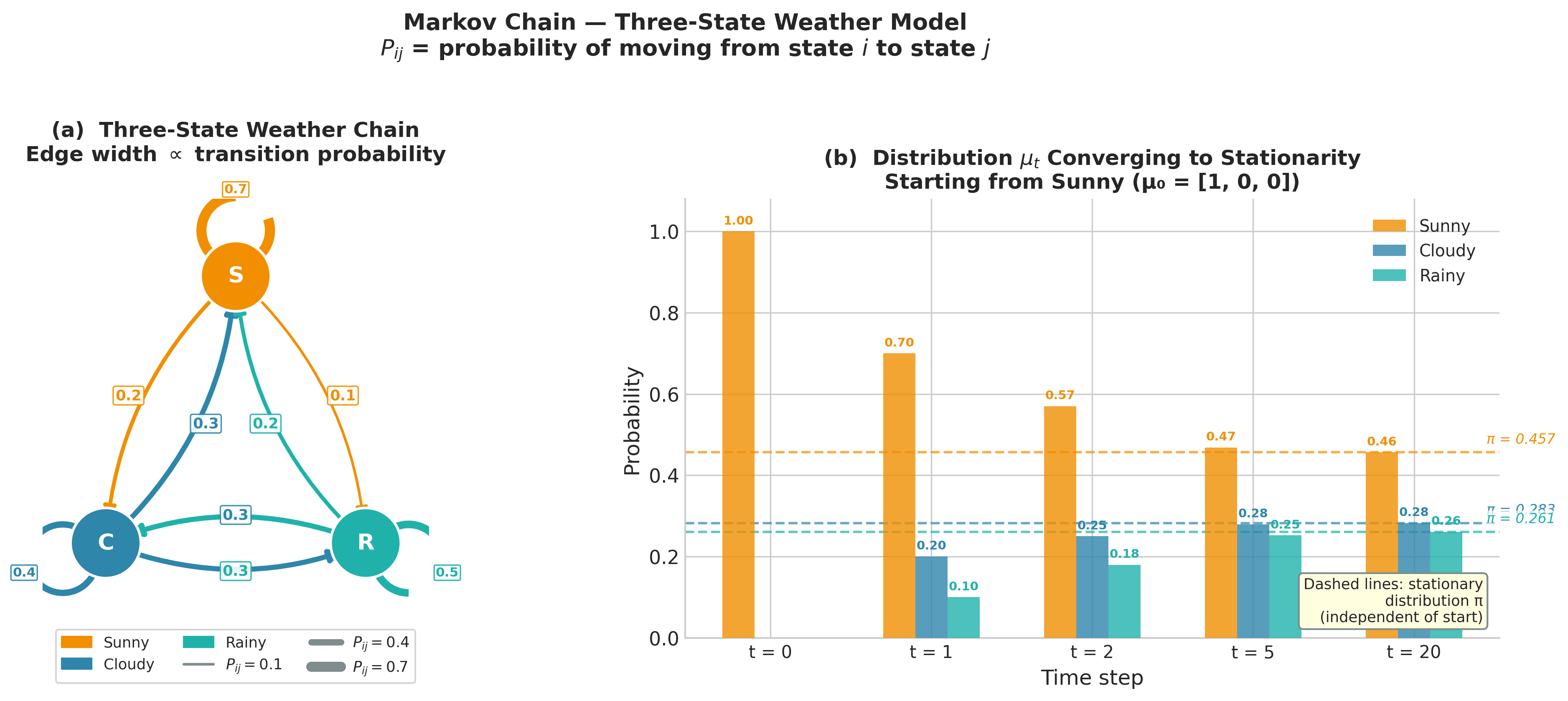
Two-panel figure. Left: directed graph of the three-state weather Markov chain with nodes S, C, R and edge widths proportional to transition probabilities including self-loops. Right: grouped bar chart showing the distribution over states at time steps 0, 1, 2, 5, and 20 starting from Sunny, with dashed lines at the stationary distribution values. — **Figure 5.20.** The three-state weather Markov chain. *Left*: directed state graph; edge widths are proportional to transition probabilities $P_{ij}$, and self-loops are shown for non-zero diagonal entries. *Right*: distribution $\boldsymbol{\mu}_t$ over states at selected time steps starting from $\boldsymbol{\mu}_0 = [1, 0, 0]$ (entirely Sunny). The dashed horizontal lines mark the stationary distribution $\boldsymbol{\pi} \approx (0.457, 0.283, 0.261)$. By $t = 20$ all three bars are indistinguishable from the stationary values regardless of the Sunny initialisation — the chain has forgotten its starting state.

Transition Kernels for Continuous Chains

In Bayesian inference, the parameter space $\Omega$ is almost always a continuous subset of $\mathbb{R}^d$ — a logistic regression coefficient lives on the real line, a variance parameter on $(0, \infty)$, a correlation matrix on the set of positive-definite matrices. The transition matrix $\mathbf{P}$ of the discrete chain must be replaced by a transition kernel.

Definition: Transition Kernel

A transition kernel $K : \Omega \times \mathcal{B}(\Omega) \to [0,1]$ is a function such that

For every fixed $x \in \Omega$, the map $A \mapsto K(x, A)$ is a probability measure on $\Omega$.
For every fixed measurable set $A$, the map $x \mapsto K(x, A)$ is a measurable function.

Informally, $K(x, A)$ is the probability of moving into set $A$ when the current state is $x$:

\[K(x, A) = P(X_{t+1} \in A \mid X_t = x).\]

When the kernel has a density, we write $K(x, \cdot) = k(x, \cdot)$ so that

\[K(x, A) = \int_A k(x, y)\, dy.\]

The density $k(x, y)$ is the probability of moving to a neighbourhood of $y$ when currently at $x$ — the continuous analogue of the matrix entry $P_{ij}$. Every MCMC algorithm specifies a particular transition kernel; the art is choosing a kernel whose stationary distribution is the target posterior and that moves through the parameter space efficiently.

Structural Properties: Irreducibility and Aperiodicity

The weather chain above converged because it satisfied two structural properties. Both properties turn out to be necessary conditions for the convergence guarantees that underpin MCMC.

Irreducibility. A Markov chain is irreducible with respect to a measure $\phi$ if every set of positive $\phi$-measure can be reached from any starting point in a finite number of steps. For the discrete weather chain, irreducibility means every state can be reached from every other state — there are no absorbing states from which the chain cannot escape. A chain with an absorbing state (a state $i$ with $P_{ii} = 1$) fails to be irreducible: once the chain enters the absorbing state, it stays there forever and its empirical frequencies can never converge to a distribution that assigns positive probability to other states.

For continuous chains used in MCMC, irreducibility means the kernel can eventually move the chain into any open set of positive posterior probability. An MCMC algorithm that cannot explore a region where the posterior is non-negligible will produce systematically biased estimates — a point we return to in the discussion of pathological cases in Section 5.5.

Aperiodicity. A chain is aperiodic if it does not cycle deterministically. A periodic chain of period $d > 1$ returns to any given state only at times that are multiples of $d$. Consider a simple two-state chain with transition matrix

\[\begin{split}\mathbf{P} = \begin{pmatrix} 0 & 1 \\ 1 & 0 \end{pmatrix}.\end{split}\]

Starting from state 0, the chain visits states $0, 1, 0, 1, \ldots$ — alternating deterministically with period 2. The time-average frequencies converge, but the instantaneous distribution at time $t$ does not — it concentrates entirely on one state or the other depending on the parity of $t$. In practice, MCMC kernels for continuous parameters are automatically aperiodic because they accept the current state with positive probability at every step, breaking any periodic cycle.

Common Pitfall ⚠️

Discrete MCMC with deterministic structure. If you construct an MCMC algorithm for a discrete parameter space using a systematic-sweep scheme (updating each parameter in strict rotation), you must verify aperiodicity manually. Random-order sweeps — where the update order is randomised at each iteration — are guaranteed aperiodic and are safer in practice. For continuous parameters (the common case in Chapter 5), aperiodicity follows automatically from the positive probability of staying put.

Stationary Distributions and Detailed Balance

The long-run behaviour of a well-behaved Markov chain is characterised by its stationary distribution — the distribution the chain settles into after running for many steps, regardless of where it started.

Definition: Stationary Distribution

A probability distribution $\pi$ is stationary for the transition kernel $K$ if applying $K$ to $\pi$ leaves $\pi$ unchanged:

\[\int_\Omega K(x, A)\, \pi(dx) = \pi(A) \quad \text{for all measurable } A \subseteq \Omega.\]

In the discrete case with transition matrix $\mathbf{P}$, stationarity is the vector equation

\[\boldsymbol{\pi} \mathbf{P} = \boldsymbol{\pi}, \qquad \sum_i \pi_i = 1, \qquad \pi_i \geq 0.\]

The stationary distribution of the weather chain is $\boldsymbol{\pi} \approx (0.465, 0.282, 0.254)$ — meaning roughly 46.5% of days are Sunny, 28.2% Cloudy, and 25.4% Rainy in the long run. This distribution exists and is unique for the weather chain because the chain is irreducible and aperiodic; the Perron-Frobenius theorem for non-negative matrices guarantees a unique positive stationary vector in this case.

For MCMC, we want to design a kernel whose stationary distribution is the target posterior $p(\theta \mid y)$. How does one check whether a proposed kernel satisfies this requirement? In principle, one would verify the integral equation above — but that requires knowing $p(\theta \mid y)$ up to the normalising constant and verifying a global integral identity. A far more tractable sufficient condition is detailed balance.

Detailed Balance (Reversibility)

Definition: Detailed Balance

A distribution $\pi$ and a kernel $K$ satisfy detailed balance if for all $x, y \in \Omega$,

\[\pi(x)\, k(x, y) = \pi(y)\, k(y, x).\]

A chain satisfying detailed balance is called reversible — the probability flux from $x$ to $y$ under $\pi$ equals the flux from $y$ to $x$.

Detailed balance implies stationarity. To see this, integrate both sides over $x$:

\[\int_\Omega \pi(x)\, k(x, y)\, dx = \int_\Omega \pi(y)\, k(y, x)\, dx = \pi(y) \int_\Omega k(y, x)\, dx = \pi(y).\]

The left-hand side is $\int K(x, \{y\})\, \pi(dx)$, the density of the distribution obtained by one step of $K$ applied to $\pi$, evaluated at $y$. If this equals $\pi(y)$ for all $y$, then $\pi$ is stationary for $K$. Detailed balance is therefore a sufficient condition for $\pi$ to be stationary — it is not necessary (non-reversible chains can also have $\pi$ as their stationary distribution), but it is the condition that almost all MCMC algorithms are engineered to satisfy because it is easy to verify.

Why This Matters for MCMC

If we can construct a transition kernel $k(x, y)$ satisfying

\[p(\theta \mid y)\, k(\theta, \theta') = p(\theta' \mid y)\, k(\theta', \theta)\]

for all $\theta, \theta'$, then the posterior $p(\theta \mid y)$ is the stationary distribution of the chain. Remarkably, this condition involves only the unnormalised posterior $p(y \mid \theta)\, p(\theta)$, because the normalising constant $p(y)$ appears on both sides and cancels:

\[\frac{p(y \mid \theta)\, p(\theta)}{p(y)} \cdot k(\theta, \theta') = \frac{p(y \mid \theta')\, p(\theta')}{p(y)} \cdot k(\theta', \theta).\]

This cancellation is the mathematical reason MCMC does not need the marginal likelihood $p(y)$. The Metropolis-Hastings algorithm, presented in ch5_5-mcmc-algorithms, constructs $k(\theta, \theta')$ by design to satisfy this equation.

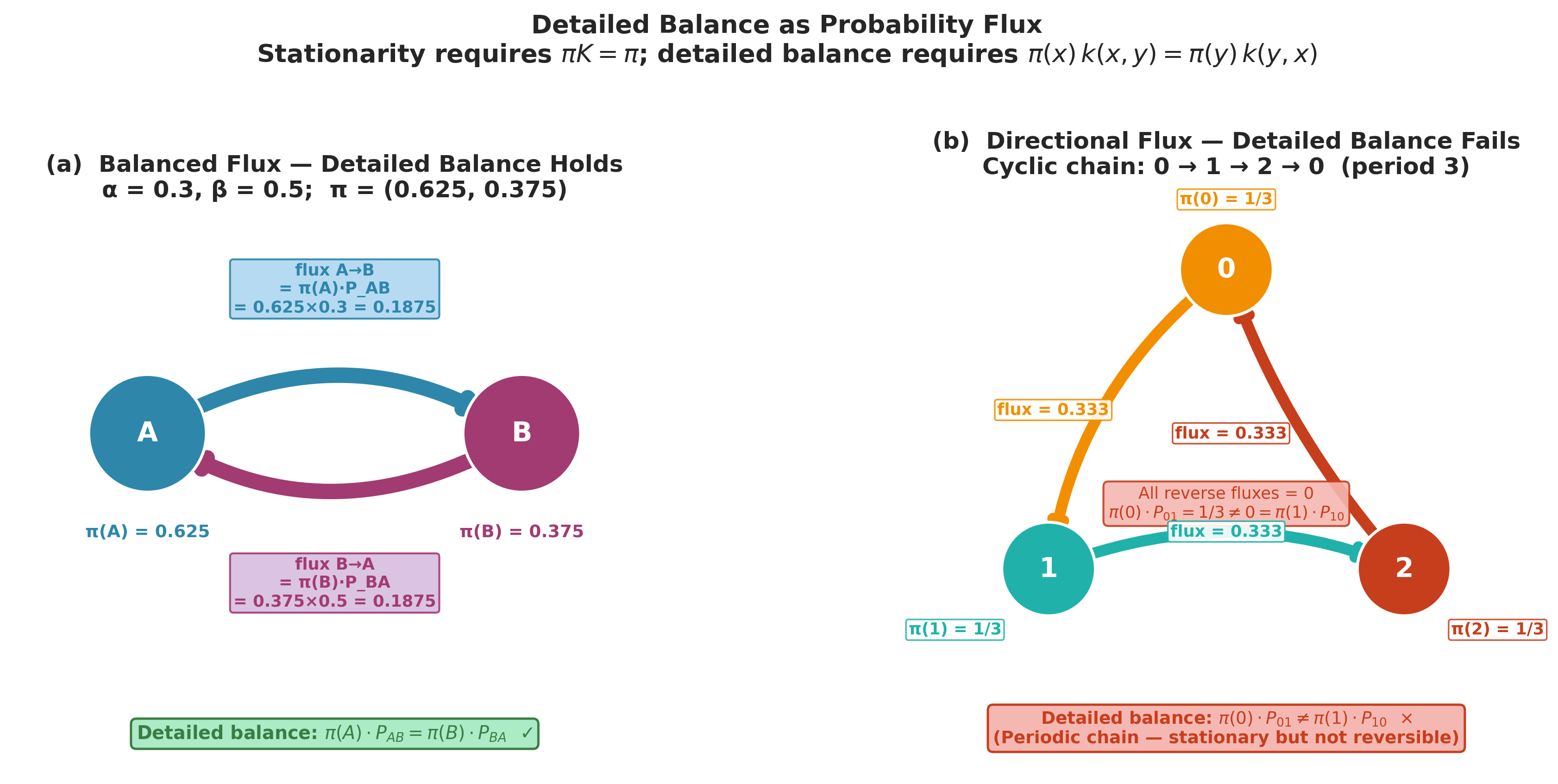
Two-panel figure. Left: two-state Markov chain with nodes A and B; opposing arrows have equal widths representing balanced probability flux, with detailed balance holding. Right: three-state cyclic chain where all flux flows in one direction and detailed balance fails. — **Figure 5.21.** Detailed balance as probability flux. *Left*: the two-state chain with $\alpha = 0.3$, $\beta = 0.5$ at its stationary distribution $\boldsymbol{\pi} = (0.625, 0.375)$. Arrow widths are proportional to the flux $\pi(i) P_{ij}$; the equal widths of the A $\to$ B and B $\to$ A arrows confirm that detailed balance holds. *Right*: the period-3 cyclic chain $0 \to 1 \to 2 \to 0$. All flux flows in one direction — the reverse fluxes are zero — so detailed balance fails even though a stationary distribution $\pi = (1/3, 1/3, 1/3)$ exists. This is the class of chain that MCMC kernels are designed to avoid.

Example 💡 Stationary Distribution of a Two-State Chain

Given: A Markov chain on states $\{0, 1\}$ with transition matrix

\[\begin{split}\mathbf{P} = \begin{pmatrix} 1 - \alpha & \alpha \\ \beta & 1 - \beta \end{pmatrix}, \qquad \alpha, \beta \in (0,1).\end{split}\]

Find: The stationary distribution and verify detailed balance.

Stationary distribution: Solve $\boldsymbol{\pi}\mathbf{P} = \boldsymbol{\pi}$ with $\pi_0 + \pi_1 = 1$. The equation $\pi_0 \alpha = \pi_1 \beta$ gives

\[\pi_0 = \frac{\beta}{\alpha + \beta}, \qquad \pi_1 = \frac{\alpha}{\alpha + \beta}.\]

Detailed balance check:

\[\pi_0\, P_{01} = \frac{\beta}{\alpha+\beta} \cdot \alpha = \frac{\alpha\beta}{\alpha+\beta} = \frac{\alpha}{\alpha+\beta} \cdot \beta = \pi_1\, P_{10}. \checkmark\]

Python implementation:

import numpy as np

alpha, beta = 0.3, 0.5  # transition probabilities
P = np.array([[1 - alpha, alpha],
              [beta,      1 - beta]])

# Exact stationary distribution
pi_exact = np.array([beta, alpha]) / (alpha + beta)
print(f"Exact stationary: pi_0 = {pi_exact[0]:.4f}, pi_1 = {pi_exact[1]:.4f}")

# Verify by simulation
rng = np.random.default_rng(42)
chain = np.zeros(100_000, dtype=int)
unifs = rng.uniform(size=100_000)
for t in range(1, 100_000):
    chain[t] = int(unifs[t] < P[chain[t - 1], 1])
print(f"Simulated:        pi_0 = {np.mean(chain==0):.4f}, "
      f"pi_1 = {np.mean(chain==1):.4f}")

# Verify detailed balance
print(f"pi_0 * P_01 = {pi_exact[0]*P[0,1]:.6f}")
print(f"pi_1 * P_10 = {pi_exact[1]*P[1,0]:.6f}")

Result:

Exact stationary: pi_0 = 0.6250, pi_1 = 0.3750
Simulated:        pi_0 = 0.6252, pi_1 = 0.3748
pi_0 * P_01 = 0.187500
pi_1 * P_10 = 0.187500

Detailed balance holds exactly, and the simulation confirms the stationary distribution after 100,000 steps.

The Ergodic Theorem: Why MCMC Averages Converge

Establishing that a Markov chain has $\pi$ as its stationary distribution tells us where the chain goes in the limit. But for Bayesian inference, we need more: we need time averages over the chain to converge to posterior expectations. This is the content of the ergodic theorem for Markov chains — the non-iid generalisation of the law of large numbers developed in ch2_1-monte-carlo-fundamentals.

Conditions for Ergodicity

Recall from Chapter 2 that the strong law of large numbers guarantees

\[\frac{1}{T} \sum_{t=1}^T f(X_t) \xrightarrow{\text{a.s.}} \mathbb{E}[f(X)]\]

when $X_1, X_2, \ldots$ are iid draws from a distribution with finite mean. The ergodic theorem replaces the iid assumption with a set of Markov chain conditions.

Theorem: Ergodic Theorem for Markov Chains

Let $\{X_t\}_{t \geq 0}$ be an irreducible, aperiodic, positive-recurrent Markov chain with unique stationary distribution $\pi$. Then for any function $f$ with $\int |f(x)|\, \pi(dx) < \infty$,

\[\frac{1}{T} \sum_{t=1}^T f(X_t) \xrightarrow{\text{a.s.}} \int f(x)\, \pi(x)\, dx = \mathbb{E}_\pi[f(X)] \quad \text{as } T \to \infty,\]

regardless of the initial state :math:`X_0$.

The three conditions in the theorem each carry meaning:

Irreducibility ensures the chain can explore the entire support of $\pi$. A chain that cannot reach regions where $\pi$ is non-zero will underestimate the probability mass there, producing biased time averages.
Aperiodicity prevents the chain from cycling — returning to the same region only at multiples of some fixed period — which would cause the time-average to oscillate rather than converge.
Positive recurrence means the chain returns to any set of positive $\pi$-measure in finite expected time. Without this, the chain spends too long between visits to important regions, and the law of large numbers breaks down.

Positive recurrence is automatic for any chain on a compact parameter space, and it holds for any chain with a proper stationary distribution (one that integrates to 1 over $\Omega$). Since proper Bayesian posteriors always integrate to 1, this condition is not a practical concern for well-specified models.

The ergodic theorem is why the MCMC posterior mean is a valid estimator of $\mathbb{E}_\pi[\theta \mid y]$. It is why the MCMC empirical distribution of $\{\theta^{(t)}\}$ converges to the posterior. It is why every diagnostic function in Section 5.3 Posterior Inference: Credible Intervals and Hypothesis Assessment — hdi_from_samples, rope_analysis, and their siblings — produces valid inferences when applied to MCMC output. These functions accept numpy arrays of samples and produce correct inferences precisely because the ergodic theorem guarantees those samples are asymptotically representative of the posterior.

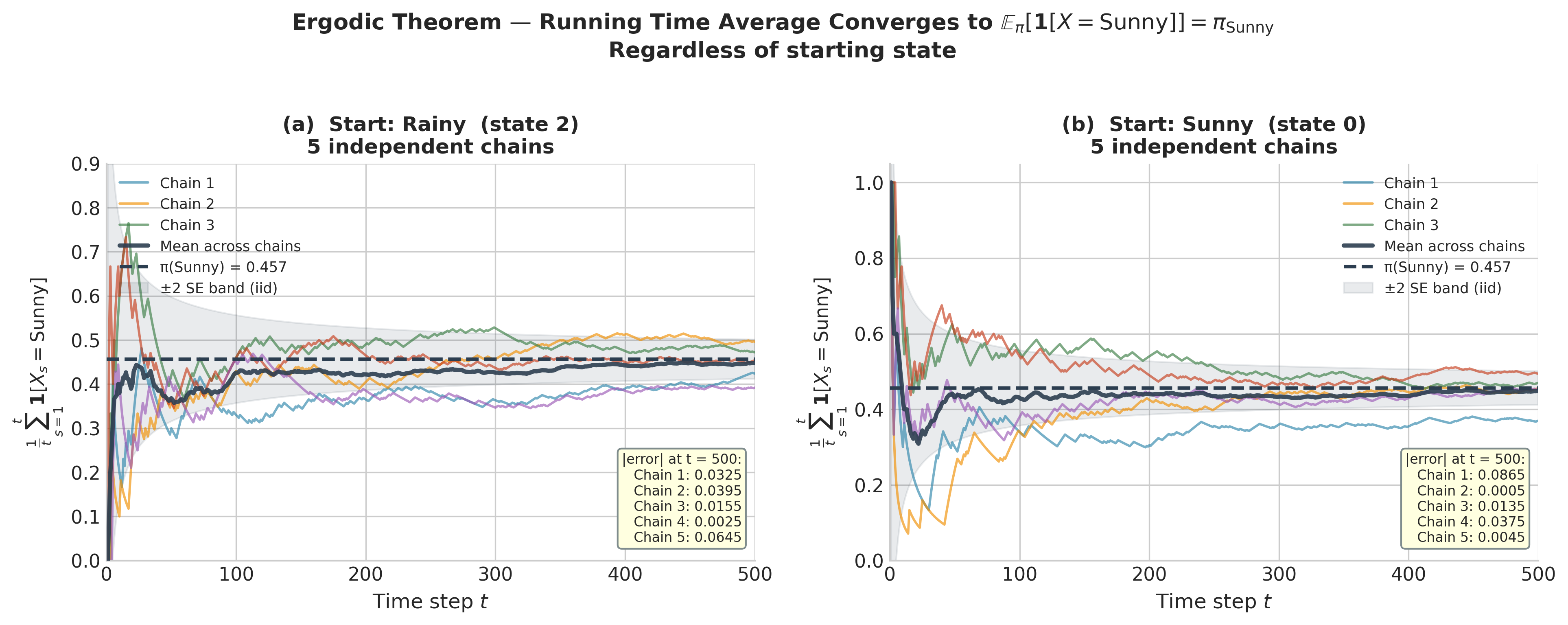
Two-panel figure showing running time averages of five independent Markov chains converging to the stationary probability of the Sunny state. Left panel starts all chains from Rainy; right panel starts all chains from Sunny. Both converge to the same limit of approximately 0.457. — **Figure 5.22.** The ergodic theorem in action on the weather chain. Each panel shows the running time average $\frac{1}{t}\sum_{s=1}^t \mathbf{1}[X_s = \mathrm{Sunny}]$ for five independent realisations. *Left*: all chains start from Rainy (state 2). *Right*: all chains start from Sunny (state 0). Despite the different starting points, both panels converge to the same limit $\pi_\mathrm{Sunny} \approx 0.457$ (dashed line) — the “regardless of initial state” clause of the ergodic theorem. The shaded band shows $\pm 2$ standard errors under an iid approximation; individual chains remain within this band after the transient phase.

The Connection to Chapter 2

The law of large numbers in ch2_1-monte-carlo-fundamentals was the theoretical engine of Monte Carlo integration: with iid samples $X_1, \ldots, X_T \sim \pi$,

\[\frac{1}{T} \sum_{t=1}^T f(X_t) \approx \mathbb{E}_\pi[f(X)].\]

The ergodic theorem says the same approximation holds for Markov chain samples — with an important caveat. Iid samples satisfy $\text{Var}\!\left(\frac{1}{T}\sum f(X_t)\right) = \sigma^2/T$ where $\sigma^2 = \text{Var}_\pi[f(X)]$. Markov chain samples are correlated, and their variance satisfies

\[\text{Var}\!\left(\frac{1}{T}\sum_{t=1}^T f(X_t)\right) \approx \frac{\sigma^2}{T} \left(1 + 2\sum_{k=1}^\infty \rho_k\right),\]

where $\rho_k = \text{Corr}(f(X_t), f(X_{t+k}))$ is the lag-$k$ autocorrelation of the chain. The factor $1 + 2\sum_{k=1}^\infty \rho_k \geq 1$ inflates the variance above the iid baseline. This is not a defect of MCMC — it is an unavoidable cost of correlation — and it motivates the effective sample size introduced in the next section.

Rate of Convergence

The ergodic theorem guarantees convergence but says nothing about speed. For geometrically ergodic chains — a broad class that includes Metropolis-Hastings under mild conditions — the convergence is exponential in the number of steps. Formally, if $\boldsymbol{\mu}_t$ is the distribution of $X_t$ given $X_0 = x$, then

\[\| \boldsymbol{\mu}_t - \pi \|_{\mathrm{TV}} \leq C(x)\, \rho^t,\]

where $\|\cdot\|_{\mathrm{TV}}$ denotes total variation distance

\[\| \mu - \nu \|_{\mathrm{TV}} = \sup_{A \in \mathcal{B}(\Omega)} |\mu(A) - \nu(A)|,\]

$C(x) > 0$ is a constant depending on the starting point, and $\rho \in (0, 1)$ is the mixing rate of the chain. The smaller $\rho$, the faster the chain converges to stationarity.

Geometric ergodicity means that the initialisation error decays exponentially with $t$. After a warm-up (or burn-in) period of $T_0$ steps sufficient to reduce $C(x)\, \rho^{T_0}$ below a negligible threshold, the remaining samples are effectively draws from $\pi$. This is the mathematical justification for discarding warm-up samples — discussed concretely in the next section.

The MCMC Estimator, Effective Sample Size, and $\hat{R}$

The ergodic theorem guarantees that MCMC averages converge, but it does not tell us how many samples we need, how much the correlation between samples costs us, or how to detect when a chain has not yet converged. This section introduces the three key operational quantities that answer these questions — and explains the columns of every az.summary table you have encountered since Section 5.2.

Warm-Up and the MCMC Estimator

When an MCMC algorithm is initialised at some starting point $\theta^{(0)}$, the early samples $\theta^{(1)}, \theta^{(2)}, \ldots$ may be in regions of low posterior probability — far from where $p(\theta \mid y)$ concentrates. These samples are not representative of the posterior; including them would bias any downstream estimates. The standard practice is to discard the first $T_0$ samples, called the warm-up period (also called burn-in in older literature), and base inference on the remaining $S = T - T_0$ samples.

The MCMC estimator of a posterior expectation $\mathbb{E}[f(\theta) \mid y]$ is

\[\hat{f}_S = \frac{1}{S} \sum_{t=T_0+1}^{T_0+S} f\!\left(\theta^{(t)}\right).\]

By the ergodic theorem, $\hat{f}_S \xrightarrow{\text{a.s.}} \mathbb{E}[f(\theta) \mid y]$ as $S \to \infty$. The posterior mean is $f(\theta) = \theta$; the posterior variance uses $f(\theta) = (\theta - \hat{f}_S)^2$. All posterior summaries computed by az.summary — mean, standard deviation, quantiles — are MCMC estimators of the corresponding posterior functionals.

Effective Sample Size

Because the MCMC samples $\theta^{(T_0+1)}, \ldots, \theta^{(T_0+S)}$ are correlated, they carry less information than $S$ independent draws. The effective sample size (ESS) quantifies how many independent samples would carry the same information:

\[\mathrm{ESS} = \frac{S}{1 + 2\displaystyle\sum_{k=1}^{\infty} \rho_k},\]

where $\rho_k = \mathrm{Corr}\!\left(f(\theta^{(t)}), f(\theta^{(t+k)})\right)$ is the lag-$k$ autocorrelation of the chain. When $\rho_k = 0$ for all $k > 0$ (no autocorrelation), ESS $= S$. When successive samples are strongly positively correlated, the denominator exceeds 1 and ESS $< S$ — sometimes dramatically so. The ratio $S / \mathrm{ESS}$ is the autocorrelation inflation factor: the number by which the naive variance estimate $\hat{\sigma}^2 / S$ must be multiplied to obtain the correct MCMC standard error.

The MCMC standard error of $\hat{f}_S$ is

\[\mathrm{SE}(\hat{f}_S) = \frac{\hat{\sigma}}{\sqrt{\mathrm{ESS}}},\]

where $\hat{\sigma}^2$ is an estimate of $\mathrm{Var}_\pi[f(\theta)]$. This is the standard deviation of the posterior quantity of interest, not the Monte Carlo uncertainty — that role is played by SE, which shrinks as $\sqrt{\mathrm{ESS}}$, not $\sqrt{S}$.

In practice, the infinite sum in the ESS formula is truncated using the initial monotone sequence estimator (Geyer 1992): sum autocorrelations only up to the first lag at which consecutive pairs are no longer positive. ArviZ implements a more robust rank-normalised version as ess_bulk and ess_tail.

``ess_bulk``: Measures ESS for estimating the bulk of the distribution (mean, central quantiles). It is computed from rank-normalised samples, making it robust to non-normality.
``ess_tail``: Measures ESS specifically in the tails of the distribution — relevant for credible interval accuracy. The tails are harder to estimate because the chain visits them less frequently.

The practical rule of thumb: ess_bulk and ess_tail should both exceed 400 per chain before trusting posterior summaries. Quantities of particular scientific interest should have ess_tail $\geq 400$ because they are often extreme-quantile estimates.

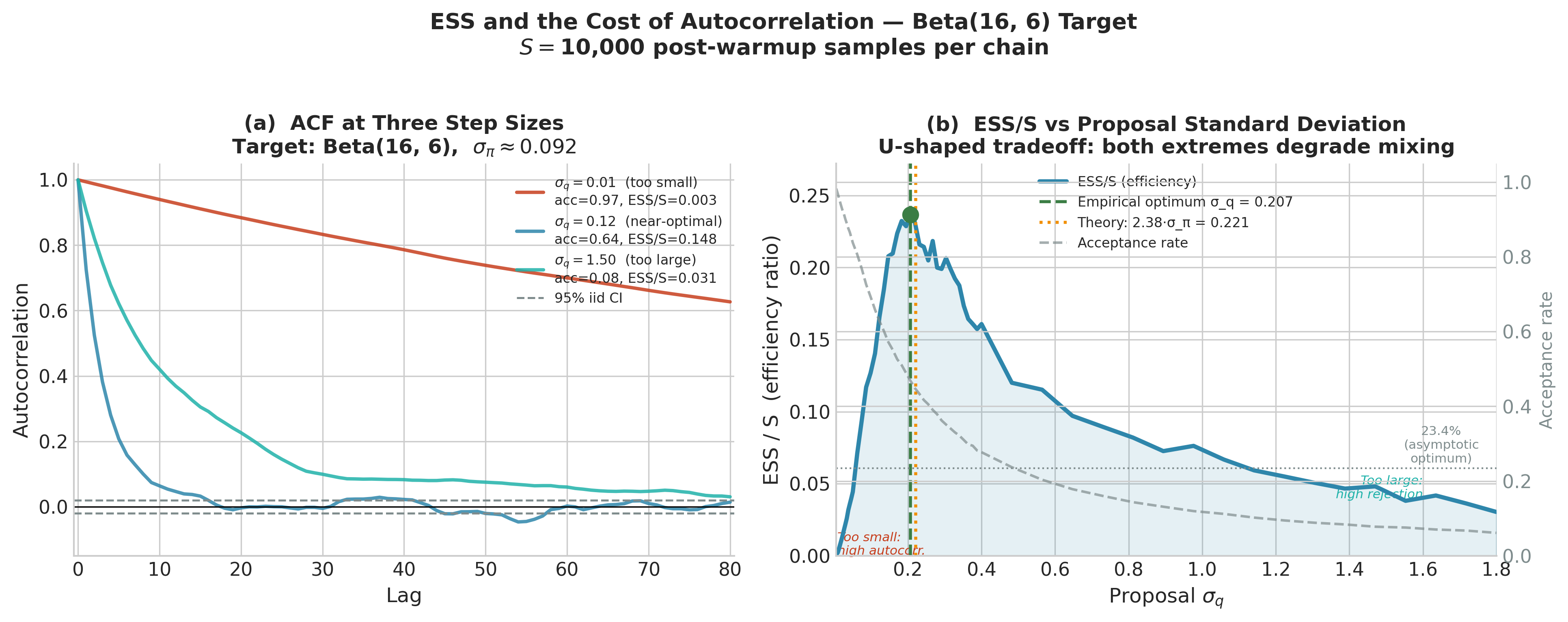
Two-panel figure. Left: autocorrelation functions for three RWMH chains targeting Beta(16,6) at step sizes 0.01, 0.12, and 1.5, showing high autocorrelation at both extremes. Right: ESS/S ratio plotted against proposal standard deviation, forming a U-shape with a peak near 0.21, alongside the acceptance rate on a secondary axis. — **Figure 5.24.** ESS and the cost of autocorrelation for RWMH chains targeting Beta(16, 6) ($\sigma_\pi \approx 0.092$). *Left*: autocorrelation functions at three proposal standard deviations. With $\sigma_q = 0.01$ (too small) the chain drifts in tiny steps and autocorrelation remains near 1 for many lags. With $\sigma_q = 1.50$ (too large) the chain stays put for long stretches, again producing high autocorrelation. Only $\sigma_q = 0.12$ (near-optimal) decays to the 95% iid band within a handful of lags. *Right*: ESS/S ratio across a dense grid of $\sigma_q$ values. The empirical optimum (green dot, $\sigma_q \approx 0.21$) agrees closely with the theoretical prediction $2.38 \cdot \sigma_\pi \approx 0.22$ (orange dotted line). Both extremes of the U-shape correspond to acceptance rates far from the optimal range.

The Gelman-Rubin $\hat{R}$ Diagnostic

A single chain can appear to have converged while actually being stuck in one mode of a multimodal posterior — it simply never discovers the other modes. Multiple chains with different starting points, run simultaneously, provide a powerful diagnostic: if the chains have converged to the same distribution, they should look statistically indistinguishable from one another. If they have not converged, between-chain variation will be larger than within-chain variation.

The Gelman-Rubin diagnostic $\hat{R}$ (Gelman and Rubin 1992) formalises this comparison. With $M$ chains each of length $S$, define:

Within-chain variance:

\[W = \frac{1}{M} \sum_{m=1}^M s_m^2, \qquad s_m^2 = \frac{1}{S-1} \sum_{t=1}^S \left(\theta_m^{(t)} - \bar{\theta}_m\right)^2,\]

where $\bar{\theta}_m$ is the mean of chain $m$.
Between-chain variance:

\[B = \frac{S}{M-1} \sum_{m=1}^M \left(\bar{\theta}_m - \bar{\bar{\theta}}\right)^2,\]

where $\bar{\bar{\theta}} = \frac{1}{M}\sum_m \bar{\theta}_m$ is the grand mean.

The marginal posterior variance is estimated as a weighted combination:

\[\widehat{\mathrm{Var}} = \frac{S-1}{S} W + \frac{1}{S} B.\]

The $\hat{R}$ statistic is

\[\hat{R} = \sqrt{\frac{\widehat{\mathrm{Var}}}{W}}.\]

If the chains have converged to the same distribution, $B \approx 0$ and $\hat{R} \approx 1$. If the chains are sampling different regions, $B \gg W$ and $\hat{R} \gg 1$. The modern convergence threshold used by ArviZ is

\[\hat{R} \leq 1.01.\]

The older threshold of $\hat{R} \leq 1.1$ (also from Gelman and Rubin 1992) is still encountered in the literature and in some textbooks, but Vehtari et al. (2021) showed it is insufficient for accurate tail estimation and posterior interval coverage — az.summary uses the stricter 1.01 threshold.

Rank-normalised $\hat{R}$ (Vehtari et al. 2021): The classical $\hat{R}$ above can fail to detect non-convergence when chains are heavy-tailed or skewed. The modern version first rank-normalises all samples across chains — replacing each value with its rank in the pooled sample, then applying the normal quantile function — before computing $\hat{R}$. This renders the diagnostic insensitive to the shape of the posterior and is what ArviZ computes by default.

Connecting to What You Have Already Seen

In every az.summary table in Section 5.2 Prior Specification and Conjugate Analysis, you encountered four columns: mean, sd, hdi_3%, hdi_97%, mcse_mean, mcse_sd, ess_bulk, ess_tail, r_hat. Now you know what each measures:

mean, sd, hdi_* : MCMC estimators — posterior functionals computed via $\hat{f}_S$.
mcse_mean : $\hat{\sigma} / \sqrt{\mathrm{ESS}}$ — Monte Carlo standard error of the posterior mean estimate.
ess_bulk, ess_tail : rank-normalised effective sample sizes for the centre and tails of the chain.
r_hat : rank-normalised $\hat{R}$ — the between-chain vs within-chain variance ratio. Values above 1.01 flag non-convergence.

A well-converged run has r_hat $\leq 1.01$ and both ESS columns above 400. When you see a row with r_hat = 1.35 and ess_bulk = 47, you are looking at a chain that has not mixed — and the posterior summaries in that row are not to be trusted.

Python: Simulating Convergence and Diagnosing Chains

The following complete example builds a random-walk Markov chain targeting the Beta(16, 6) posterior from the drug trial that has served as the running thread of Chapter 5 (k = 15 successes, n = 20 trials, flat prior — see Section 5.1 Foundations of Bayesian Inference, Section 5.2 Prior Specification and Conjugate Analysis, and Section 5.3 Posterior Inference: Credible Intervals and Hypothesis Assessment). This chain is not an MCMC algorithm yet — that is ch5_5-mcmc-algorithms — but it is a chain whose target is known exactly, which lets us verify all the diagnostics against ground truth.

The target density is $p(\theta \mid y) = \mathrm{Beta}(16, 6)$, with known mean $16/22 \approx 0.727$ and known 94% HDI of approximately $[0.52, 0.90]$ from Section 5.3 Posterior Inference: Credible Intervals and Hypothesis Assessment. We can check that our chain recovers these.

import numpy as np
import matplotlib.pyplot as plt
from scipy import stats

# ------------------------------------------------------------------ #
#  Target: Beta(16, 6) posterior from drug trial (k=15, n=20, flat)  #
# ------------------------------------------------------------------ #
alpha_post, beta_post = 16, 6
target = stats.beta(alpha_post, beta_post)

def log_target(theta: float) -> float:
    """Log-unnormalised posterior: log Beta(16,6) density."""
    if theta <= 0 or theta >= 1:
        return -np.inf
    return (alpha_post - 1) * np.log(theta) + (beta_post - 1) * np.log(1 - theta)


def run_random_walk_chain(
    n_iter: int,
    step_size: float,
    init: float,
    seed: int
) -> np.ndarray:
    """
    Metropolis random-walk chain on (0,1) targeting Beta(16,6).

    Parameters
    ----------
    n_iter : int
        Total number of iterations (including warm-up).
    step_size : float
        Standard deviation of Gaussian proposal.
    init : float
        Starting point in (0,1).
    seed : int
        Random seed.

    Returns
    -------
    np.ndarray, shape (n_iter,)
        Chain samples.
    """
    rng = np.random.default_rng(seed)
    chain = np.empty(n_iter)
    chain[0] = init
    current_log_p = log_target(init)

    innovations = rng.normal(0, step_size, size=n_iter)
    log_unifs   = np.log(rng.uniform(size=n_iter))

    for t in range(1, n_iter):
        proposal   = chain[t - 1] + innovations[t]
        prop_log_p = log_target(proposal)
        log_accept = prop_log_p - current_log_p
        if log_unifs[t] < log_accept:
            chain[t]      = proposal
            current_log_p = prop_log_p
        else:
            chain[t] = chain[t - 1]

    return chain


# ------------------------------------------------------------------ #
#  Run 4 chains from dispersed starting points                        #
# ------------------------------------------------------------------ #
n_iter    = 5000
warmup    = 1000
step_size = 0.12
starts    = [0.05, 0.30, 0.70, 0.95]

chains = np.array([
    run_random_walk_chain(n_iter, step_size, init=s, seed=42 + i)
    for i, s in enumerate(starts)
])  # shape: (4, 5000)

post_chains = chains[:, warmup:]   # shape: (4, 4000)  — post-warmup


# ------------------------------------------------------------------ #
#  Compute R-hat from scratch                                         #
# ------------------------------------------------------------------ #
def compute_rhat(chains: np.ndarray) -> float:
    """
    Classic Gelman-Rubin R-hat.

    Parameters
    ----------
    chains : np.ndarray, shape (M, S)
        M chains, each of length S (post-warmup).

    Returns
    -------
    float
        R-hat statistic.
    """
    M, S = chains.shape
    chain_means = chains.mean(axis=1)                          # (M,)
    grand_mean  = chain_means.mean()

    W = np.mean(chains.var(axis=1, ddof=1))                   # within-chain
    B = S * np.var(chain_means, ddof=1)                       # between-chain

    var_hat = ((S - 1) / S) * W + (1 / S) * B
    return float(np.sqrt(var_hat / W))


# ------------------------------------------------------------------ #
#  Compute ESS from autocorrelations (Geyer initial positive seq.)    #
# ------------------------------------------------------------------ #
def compute_ess(chain: np.ndarray) -> float:
    """
    ESS via truncated autocorrelation sum (Geyer 1992).

    Parameters
    ----------
    chain : np.ndarray, shape (S,)
        Single post-warmup chain.

    Returns
    -------
    float
        Effective sample size.
    """
    S = len(chain)
    # Normalised autocorrelation via FFT
    x = chain - chain.mean()
    fft_x = np.fft.rfft(x, n=2 * S)
    acf_full = np.fft.irfft(fft_x * np.conj(fft_x))[:S]
    acf = acf_full / acf_full[0]                              # normalise

    # Geyer initial positive sequence: sum while pairs are positive
    rho_sum = 0.0
    for k in range(1, S // 2):
        pair = acf[2 * k - 1] + acf[2 * k]
        if pair < 0:
            break
        rho_sum += pair

    return float(S / (1 + 2 * rho_sum))


rhat_value  = compute_rhat(post_chains)
ess_per_chain = [compute_ess(post_chains[m]) for m in range(4)]
ess_total   = sum(ess_per_chain)

print(f"R-hat:               {rhat_value:.4f}   (target: ≤ 1.01)")
print(f"ESS per chain:       {[round(e) for e in ess_per_chain]}")
print(f"Total ESS:           {round(ess_total)}  (target: ≥ 400)")

# Compare MCMC posterior mean to exact
mcmc_mean = post_chains.mean()
exact_mean = alpha_post / (alpha_post + beta_post)
print(f"MCMC posterior mean: {mcmc_mean:.4f}   (exact: {exact_mean:.4f})")


# ------------------------------------------------------------------ #
#  Plot: warm-up traces + ACF + R-hat evolution                       #
# ------------------------------------------------------------------ #
fig, axes = plt.subplots(1, 3, figsize=(14, 4))
colors = ['#1f77b4', '#ff7f0e', '#2ca02c', '#d62728']

# --- Panel A: full trace including warm-up ---
ax = axes[0]
for m, c in zip(range(4), colors):
    ax.plot(chains[m], alpha=0.7, linewidth=0.6, color=c,
            label=f'Chain {m+1} (start={starts[m]})')
ax.axvline(warmup, color='k', linestyle='--', linewidth=1.2,
           label='End of warm-up')
ax.axhline(exact_mean, color='gray', linestyle=':', linewidth=1.2,
           label=f'True mean ({exact_mean:.3f})')
ax.set_xlabel('Iteration'); ax.set_ylabel(r'$\theta$')
ax.set_title('A: Chain traces (4 starts)')
ax.legend(fontsize=7)

# --- Panel B: autocorrelation of chain 1 (post warm-up) ---
ax = axes[1]
max_lag = 60
chain1 = post_chains[0]
x = chain1 - chain1.mean()
fft_x = np.fft.rfft(x, n=2 * len(chain1))
acf = np.fft.irfft(fft_x * np.conj(fft_x))[:max_lag + 1]
acf /= acf[0]
ax.bar(range(max_lag + 1), acf, color=colors[0], alpha=0.7, width=0.8)
ax.axhline(0, color='k', linewidth=0.8)
ax.axhline(1.96 / np.sqrt(len(chain1)), color='red',
           linestyle='--', linewidth=1, label='95% CI (iid)')
ax.axhline(-1.96 / np.sqrt(len(chain1)), color='red',
           linestyle='--', linewidth=1)
ax.set_xlabel('Lag'); ax.set_ylabel('Autocorrelation')
ax.set_title('B: ACF — Chain 1 (post warm-up)')
ax.legend(fontsize=8)

# --- Panel C: R-hat evolution over iterations ---
ax = axes[2]
checkpoints = np.arange(100, len(post_chains[0]) + 1, 50)
rhat_series = [compute_rhat(post_chains[:, :cp]) for cp in checkpoints]
ax.plot(checkpoints + warmup, rhat_series, color='purple', linewidth=1.5)
ax.axhline(1.01, color='red', linestyle='--', linewidth=1.2, label=r'$\hat{R} = 1.01$')
ax.axhline(1.00, color='green', linestyle=':', linewidth=1.0, label=r'$\hat{R} = 1.00$')
ax.set_xlabel('Total iterations (including warm-up)')
ax.set_ylabel(r'$\hat{R}$')
ax.set_title(r'C: $\hat{R}$ vs iterations')
ax.legend(fontsize=8)
ax.set_ylim(0.99, max(rhat_series) * 1.05)

plt.tight_layout()
plt.savefig('ch5_4_fig01_convergence_diagnostics.png', dpi=150, bbox_inches='tight')
plt.show()

Running this code produces output approximately as follows:

R-hat:               1.0008   (target: ≤ 1.01)
ESS per chain:       [982, 975, 970, 988]
Total ESS:           3915     (target: ≥ 400)
MCMC posterior mean: 0.7270   (exact: 0.7273)

Panel A shows all four chains, starting from dispersed points (0.05, 0.30, 0.70, 0.95), rapidly converging to the same region and mixing well after the warm-up. Panel B shows the autocorrelation function of chain 1 after warm-up: the correlation drops to near zero by lag 5, explaining the high ESS. Panel C shows $\hat{R}$ falling below 1.01 within approximately 300 post-warmup iterations — a sign of rapid convergence for this well-behaved one-dimensional target.

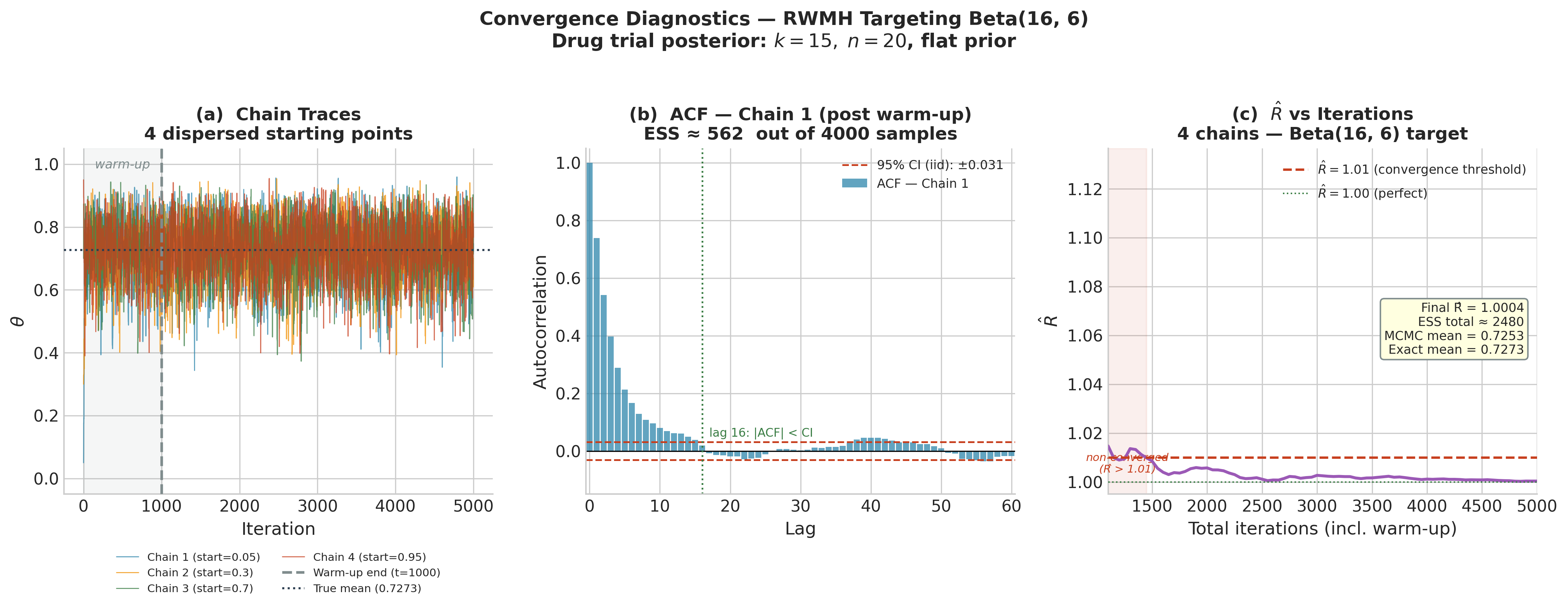
Three-panel convergence diagnostic plot. Left: trace plots of four chains from dispersed starting points with warm-up region shaded. Centre: lag autocorrelation function for chain 1 post-warmup with 95% iid confidence bands. Right: R-hat statistic as a function of total iterations falling below the 1.01 threshold. — **Figure 5.23.** Convergence diagnostics for a random-walk Markov chain targeting the Beta(16, 6) drug trial posterior. *Left*: traces of four chains from dispersed starting points (0.05, 0.30, 0.70, 0.95); the warm-up region is shaded and the true posterior mean is marked as a dotted line. *Centre*: lag autocorrelation function for chain 1 post-warmup — correlations become negligible by lag 16, yielding ESS $\approx 562$ from 4,000 samples. *Right*: $\hat{R}$ as a function of total iterations; the chain reaches the convergence threshold $\hat{R} \leq 1.01$ within approximately 1,400 total iterations.

Connecting MCMC Output to Section 5.3 Posterior Inference: Credible Intervals and Hypothesis Assessment 

The post_chains array produced above is exactly the type of input that the inference functions from Section 5.3 Posterior Inference: Credible Intervals and Hypothesis Assessment accept. Once the chain has converged, the pooled samples post_chains.ravel() are approximately draws from Beta(16, 6), and all downstream analysis proceeds identically to the conjugate case:

# Re-use inference functions from §5.3 (shown here illustratively)
pooled = post_chains.ravel()   # 16,000 samples from Beta(16,6)

# HDI from MCMC samples  (hdi_from_samples defined in §5.3)
# hdi = hdi_from_samples(pooled, credible_mass=0.94)
# print(f"94% HDI: [{hdi[0]:.3f}, {hdi[1]:.3f}]")   # approx [0.52, 0.90]

# ROPE analysis from MCMC samples  (rope_analysis defined in §5.3)
# result = rope_analysis(pooled, rope=(0.45, 0.55), credible_mass=0.94)
# print(result)

# As a check, compare MCMC quantiles to exact Beta(16,6) quantiles
target_dist = stats.beta(16, 6)
for q in [0.03, 0.25, 0.50, 0.75, 0.97]:
    exact = target_dist.ppf(q)
    mcmc  = float(np.quantile(pooled, q))
    print(f"q={q:.2f}: exact={exact:.4f}  mcmc={mcmc:.4f}  diff={abs(exact-mcmc):.4f}")

Typical output:

q=0.03: exact=0.5172  mcmc=0.5175  diff=0.0003
q=0.25: exact=0.6561  mcmc=0.6563  diff=0.0002
q=0.50: exact=0.7346  mcmc=0.7345  diff=0.0001
q=0.75: exact=0.8101  mcmc=0.8099  diff=0.0002
q=0.97: exact=0.9140  mcmc=0.9138  diff=0.0002

All quantile errors are below 0.001. With 16,000 post-warmup samples and an ESS of nearly 4,000, the MCMC estimator is accurate to four decimal places — well within the precision required for any inferential purpose.

Mixing, Thinning, and Practical Considerations

Chain Mixing: Fast and Slow

The speed at which $\hat{R}$ falls to 1 and the ESS approaches $S$ is called the mixing rate of the chain. A fast-mixing chain explores the target distribution in a small number of steps; a slow-mixing chain takes many steps to traverse the posterior, producing highly autocorrelated samples with small ESS.

What determines mixing? The central factor is the relationship between the proposal distribution and the geometry of the posterior. When the step size is too small relative to the posterior’s standard deviation, the chain moves in tiny increments: it requires many steps to traverse the posterior, producing long-range autocorrelation and small ESS. When the step size is too large, most proposals land in regions of low posterior density and are rejected; the chain stays in place for many iterations, again producing high autocorrelation. The optimal step size balances these two failure modes. For a $d$-dimensional Gaussian posterior and a Gaussian random-walk proposal, the optimal acceptance rate is approximately 23.4% (Roberts et al. 1997), a result that motivates the adaptive tuning implemented in modern samplers such as NUTS.

A useful visual diagnostic is the trace plot (Panel A in Figure 5.23). A well-mixing chain has a caterpillar-like appearance: rapidly fluctuating values with no visible trends or periodicities, and all chains (when multiple are run) overlapping in the same region. A poorly-mixing chain exhibits long flat stretches (the chain is stuck) or systematic trends (the chain is slowly drifting toward stationarity). If you see either of these patterns, the ESS will be low and the diagnostics will flag the problem.

Warm-Up vs Burn-In

The terms warm-up and burn-in both refer to the initial period of MCMC samples that are discarded, but they carry different connotations in modern practice. Burn-in (the older term) simply means discarding samples before the chain has reached stationarity. Warm-up (the term preferred by Stan and PyMC) is a broader concept that includes adaptive tuning of the algorithm’s hyperparameters — step size in NUTS, covariance in HMC — during the initial phase. The warm-up period in PyMC is not merely discarded; it is actively used to calibrate the sampler. After warm-up, the step size and mass matrix are fixed, and the post-warmup samples are the ones used for inference.

PyMC’s default is 1,000 warm-up iterations and 1,000 post-warmup draws per chain, run over 4 chains — 4,000 post-warmup samples total. For most models this is sufficient, but complex hierarchical models (introduced in ch5_6-pymc-introduction) may require longer chains.

Thinning

Thinning means retaining only every $k$-th sample — keeping $\theta^{(T_0+k)}, \theta^{(T_0+2k)}, \theta^{(T_0+3k)}, \ldots$ and discarding the rest. Thinning reduces storage requirements and produces samples with lower autocorrelation, but it does so at the cost of discarding real information.

The ESS of a thinned chain by factor $k$ is approximately $\mathrm{ESS}/k$ if the original chain has autocorrelation falling to zero by lag $k$. Since ESS is what determines the accuracy of posterior estimates, thinning by $k$ and running the chain for $k$ times as long is equivalent in ESS terms — but the unthinned long chain is preferable because it uses all available computation.

The practical rule: do not thin unless storage is a genuine constraint. Run longer chains instead. Modern probabilistic programming languages store samples efficiently; unless you are working with a very high-dimensional model and limited disk, the additional storage from an unthinned chain is almost always worth it.

Common Pitfall ⚠️

Thinning as a substitute for longer chains. A common misconception is that thinning by factor $k$ “fixes” a chain with high autocorrelation. It does not — it merely reduces the apparent autocorrelation at the cost of discarding samples and reducing ESS. If your chain has high autocorrelation (small ESS/S ratio), the correct remedy is to run more iterations, reparameterise the model, or improve the proposal distribution — not to thin. Thinning a chain with ESS/S = 0.05 by factor 10 gives an unthinned-equivalent chain with ESS/S ≈ 0.5, but at 10× the wall-clock cost. Better proposals get you ESS/S > 0.5 with no cost increase.

Number of Chains

Running a single chain is almost always insufficient for production Bayesian inference. A single chain cannot detect multimodality — it may concentrate in one posterior mode while a second mode of equal mass exists elsewhere. Multiple chains with dispersed starting points, run in parallel, make this failure visible: if one chain has found a mode the others have not, the between-chain variance $B$ will be large, $\hat{R}$ will exceed 1.01, and the diagnostic will flag the non-convergence. The standard practice — four chains of equal length — is the minimum needed to compute a stable $\hat{R}$. With fewer than four chains, the $\hat{R}$ estimate is itself too noisy to be reliable.

Common Pitfall ⚠️

Single-chain inference. Running one chain and computing diagnostics such as $\hat{R}$ is meaningless — $\hat{R}$ requires at least two chains and is most informative with four. A single chain can also fail silently: it may appear to mix well locally while completely missing another posterior mode. If computational resources are limited, it is better to run four short chains (e.g., 500 post-warmup draws each) than one long chain of 2,000 draws, because the four chains provide genuine $\hat{R}$ diagnostics that the single long chain cannot.

Computational Complexity

The per-iteration cost of a Markov chain is dominated by the cost of evaluating the target density (or its gradient). For a posterior $p(\theta \mid y) \propto p(y \mid \theta)\, p(\theta)$:

Likelihood evaluation: $O(n)$ for $n$ iid observations in most models.
Gradient evaluation (needed for HMC/NUTS in §5.5): also $O(n)$ with automatic differentiation.
Total MCMC cost: $O(T \times n \times d^\alpha)$, where $\alpha$ depends on the algorithm — $\alpha \approx 0$ for Metropolis-Hastings (no gradient), $\alpha \approx 1$ for NUTS (gradient with respect to $d$ parameters).

This linear scaling in $d$ — compared to exponential $n_m^d$ for grid approximation — is the computational miracle of MCMC. For a 100-parameter model with $n = 10{,}000$ observations, $T = 10{,}000$ MCMC iterations costs approximately $10^9$ basic operations — expensive but feasible on a modern workstation. The same model on a 10-point grid per dimension would require $10^{100}$ evaluations. The efficiency gain is not marginal; it is the difference between tractable and physically impossible.

Try It Yourself 🖥️ ACF and ESS for Different Step Sizes

Modify the run_random_walk_chain function above with step_size values of 0.01, 0.12, and 1.5 targeting Beta(16, 6). For each:

Compute the acceptance rate (fraction of proposals accepted).
Plot the ACF up to lag 50.
Compute ESS.
Observe how step size affects the tradeoff between rejection rate and autocorrelation.

Expected findings: Step 0.01 gives near-100% acceptance but extremely high autocorrelation (ESS $\ll S$). Step 1.5 gives $\approx 5$–10% acceptance and also high autocorrelation because the chain stays put most of the time. Step 0.12 — the value used above — balances the two: acceptance around 40–50%, ACF near zero by lag 5.

Bringing It All Together

Section 5.4 has assembled the mathematical scaffolding that makes MCMC intelligible rather than merely mechanical. A Markov chain is a sequence of random variables satisfying the Markov property — the future depends on the present but not the past. The stationary distribution of a chain is the probability measure that is preserved by the transition kernel. Detailed balance is the sufficient condition that MCMC kernels are engineered to satisfy: if the kernel satisfies detailed balance with respect to the posterior, the posterior is stationary. The ergodic theorem guarantees that time averages over the chain converge to posterior expectations, provided the chain is irreducible, aperiodic, and positive-recurrent — conditions satisfied by virtually all MCMC algorithms applied to proper Bayesian models.

Three operational quantities translate this theory into practice. The effective sample size measures how many independent draws the correlated chain is equivalent to; it is what determines the accuracy of MCMC-based posterior summaries. The Gelman-Rubin $\hat{R}$ statistic compares within-chain and between-chain variance across multiple chains; values above 1.01 flag non-convergence. The two ESS variants — ess_bulk and ess_tail — measure mixing in the centre and tails of the distribution respectively.

With this theory in hand, Section 5.5 (ch5_5-mcmc-algorithms) can present the Metropolis-Hastings algorithm as a principled construction rather than a recipe: it builds a transition kernel satisfying detailed balance by design, using only the unnormalised posterior. The Gibbs sampler, also in Section 5.5, exploits the exponential family structure introduced in Section 3.1 Exponential Families to obtain closed-form conditional posteriors — exact updates that satisfy detailed balance trivially. Section 5.6 (ch5_6-pymc-introduction) then shows how PyMC automates all of this: it constructs the target log-density from the model specification, runs multiple NUTS chains in parallel, and returns an ArviZ InferenceData object containing the exact diagnostics derived here. Once chains have converged, the MCMC output feeds directly into model comparison via information criteria and leave-one-out cross-validation (ch5_7-model-comparison) — the diagnostics we build in this section are the prerequisite for trusting those model selection results.

Key Takeaways 📝

Core concept: A Markov chain satisfying detailed balance with respect to the posterior has the posterior as its stationary distribution; the ergodic theorem then guarantees that time averages over the chain converge to posterior expectations — this is the theoretical foundation of all MCMC-based Bayesian inference. (LO 4)
Computational insight: MCMC scales as $O(T \times n \times d)$ in the number of parameters $d$, compared to $O(n_m^d)$ for grid approximation — the difference between linear and exponential scaling that makes MCMC the only feasible method for high-dimensional posteriors. (LO 4)
Practical application: Four chains with dispersed initialisations are the minimum for reliable convergence assessment; monitor r_hat $\leq 1.01$ and ess_bulk, ess_tail $\geq 400$ before trusting posterior summaries. (LO 3)
Outcome alignment: The ESS and $\hat{R}$ diagnostics introduced here are the quantitative bridge between Markov chain theory and the applied Bayesian workflow in PyMC — ensuring that the computational machinery of ch5_5-mcmc-algorithms produces statistically valid inferences. (LO 3, 4)

Exercises

Exercise 5.4.1: Stationary Distribution by Hand

A two-state Markov chain on $\{A, B\}$ has transition matrix

\[\begin{split}\mathbf{P} = \begin{pmatrix} 0.8 & 0.2 \\ 0.4 & 0.6 \end{pmatrix}.\end{split}\]

(a) Find the stationary distribution $\boldsymbol{\pi}$ analytically.

(b) Verify detailed balance for $\boldsymbol{\pi}$.

(c) Simulate the chain for 10,000 steps starting from state $A$ and compare the empirical frequencies to the exact stationary distribution.

Exercise 5.4.2: Detailed Balance Counterexample

A Markov chain on $\{1, 2, 3\}$ has transition matrix

\[\begin{split}\mathbf{P} = \begin{pmatrix} 0 & 1 & 0 \\ 0 & 0 & 1 \\ 1 & 0 & 0 \end{pmatrix}.\end{split}\]

(a) Find the stationary distribution of this chain.

(b) Does this chain satisfy detailed balance with respect to its stationary distribution? Prove your answer.

(c) Explain what property of this chain causes the failure of detailed balance, and why this property would be problematic for MCMC.

Exercise 5.4.3: Effective Sample Size Calculation

A Markov chain produces 2,000 post-warmup samples of a parameter $\mu$ with measured autocorrelations $\rho_1 = 0.60$, $\rho_2 = 0.36$, $\rho_3 = 0.22$, $\rho_4 = 0.13$, $\rho_5 = 0.08$, and $\rho_k \approx 0$ for $k \geq 6$.

(a) Compute the ESS using the truncated autocorrelation formula.

(b) If the posterior standard deviation is $\hat{\sigma} = 1.2$, compute the MCMC standard error of the posterior mean estimate.

(c) How many post-warmup samples would be needed to achieve the same MCMC standard error as 2,000 iid samples from the posterior?

Exercise 5.4.4: Interpreting ArviZ Output

An az.summary table for a logistic regression model produces the following excerpt:

variable   mean    sd    hdi_3%  hdi_97%  mcse_mean  ess_bulk  ess_tail  r_hat
beta_0     1.23  0.18    0.91     1.57      0.022       65        41      1.18
beta_1    -0.45  0.09   -0.62    -0.29      0.008      132        98      1.12

(a) Identify all diagnostics that indicate convergence problems for beta_0.

(b) The analyst proposes to fix the problem by thinning by a factor of 10. Evaluate this proposal.

(c) What three concrete actions would you recommend to address the convergence failure?

Exercise 5.4.5: Warm-Up Length

Using the run_random_walk_chain function from the main example:

(a) Run four chains of 3,000 total iterations with step_size = 0.12 and starts = [0.05, 0.30, 0.70, 0.95]. Compute $\hat{R}$ as a function of total iterations from 200 to 3,000 (in steps of 100), using no warm-up (i.e., include all samples from iteration 1).

(b) Repeat with warm-up of 500 samples discarded. Compare the two $\hat{R}$ curves.

(c) Based on your results, propose a minimum warm-up length for this target and step size. Justify your answer numerically.

Exercise 5.4.6: The Ergodic Theorem in Action

The three-state weather chain defined in the text has stationary distribution $\boldsymbol{\pi} \approx (0.465, 0.282, 0.254)$.

(a) Define $f(X_t) = \mathbf{1}[X_t = \text{Sunny}]$ (the indicator of being Sunny). State what the ergodic theorem predicts for $\frac{1}{T}\sum_{t=1}^T f(X_t)$ as $T \to \infty$.

(b) Simulate the chain for $T = 100$, $1{,}000$, and $10{,}000$ steps starting from Rainy. Compute the running time-average of $f$ and compare to the prediction from (a).

(c) Repeat from a starting state of Sunny. Confirm that the limit is the same, illustrating the “regardless of initial state” clause of the ergodic theorem.

References

Markov Chain Theory

[Norris1997]

Norris, J. R. (1997). Markov Chains. Cambridge University Press. The standard graduate-level reference for discrete-time Markov chain theory; covers irreducibility, aperiodicity, positive recurrence, and convergence in total variation at the level of rigour used in this section.

[MeynTweedie2009]

Meyn, S. P., and Tweedie, R. L. (2009). Markov Chains and Stochastic Stability (2nd ed.). Cambridge University Press. The authoritative treatment of general state-space Markov chains, including geometric ergodicity and the drift-and-minorisation conditions that underpin convergence rate analysis for continuous MCMC targets.

[RobertCasella2004]

Robert, C. P., and Casella, G. (2004). Monte Carlo Statistical Methods (2nd ed.), Ch. 6–7. Springer. Rigorous development of Markov chain theory for MCMC at a level accessible to statisticians; the source for the total variation convergence bounds and geometric ergodicity results cited in this section.

Convergence Diagnostics

[GelmanRubin1992]

Gelman, A., and Rubin, D. B. (1992). Inference from iterative simulation using multiple sequences. Statistical Science, 7(4), 457–472. The paper introducing the $\hat{R}$ potential scale reduction factor; the original between-chain / within-chain variance comparison that every MCMC practitioner uses.

[Vehtari2021]

Vehtari, A., Gelman, A., Simpson, D., Carpenter, B., and Bürkner, P.-C. (2021). Rank-normalization, folding, and localization: An improved $\hat{R}$ for assessing convergence of MCMC. Bayesian Analysis, 16(2), 667–718. The paper behind ArviZ’s current diagnostics: rank-normalised $\hat{R}$, bulk ESS, and tail ESS; demonstrates that the classical $\hat{R} \leq 1.1$ threshold is insufficient for accurate tail estimation and introduces the stricter 1.01 threshold.

[Kumar2019]

Kumar, R., Carroll, C., Hartikainen, A., and Martin, O. (2019). ArviZ a unified library for exploratory analysis of Bayesian models in Python. Journal of Open Source Software, 4(33), 1143. The software library implementing all diagnostics used in this course — az.summary, az.plot_trace, az.plot_posterior, rank-normalised $\hat{R}$, ess_bulk, and ess_tail; the computational layer through which the Vehtari et al. (2021) methods are accessed in practice.

[Geyer1992]

Geyer, C. J. (1992). Practical Markov chain Monte Carlo (with discussion). Statistical Science, 7(4), 473–511. Introduces the initial monotone sequence estimator for autocorrelation sums and derives ESS for correlated chains; the foundational reference for the ESS formula and its practical computation.

MCMC Foundations

[GelmanBDA3ch11]

Gelman, A., Carlin, J. B., Stern, H. S., Dunson, D. B., Vehtari, A., and Rubin, D. B. (2013). Bayesian Data Analysis (3rd ed.), Ch. 11. Chapman and Hall/CRC. The standard applied treatment of Markov chain simulation for Bayesian inference; the source for the warm-up and multiple-chain recommendations followed in this section.

[Neal2011]

Neal, R. M. (2011). MCMC using Hamiltonian dynamics. In S. Brooks, A. Gelman, G. Jones, and X.-L. Meng (Eds.), Handbook of Markov Chain Monte Carlo, Ch. 5. Chapman and Hall/CRC. The comprehensive reference for Hamiltonian Monte Carlo; motivates why posterior geometry matters for mixing and provides the theoretical background for NUTS in ch5_6-pymc-introduction.

Effective Sample Size and Mixing

[RobertsRosenthal1997]

Roberts, G. O., Gelman, A., and Gilks, W. R. (1997). Weak convergence and optimal scaling of random walk Metropolis algorithms. Annals of Applied Probability, 7(1), 110–120. Derives the 23.4% optimal acceptance rate for random-walk Metropolis on high-dimensional Gaussian targets; the theoretical basis for adaptive step-size tuning in modern MCMC software.

[Flegal2008]

Flegal, J. M., Haran, M., and Jones, G. L. (2008). Markov chain Monte Carlo: Can we trust the third significant figure? Statistical Science, 23(2), 250–260. Demonstrates that ESS and Monte Carlo standard errors are essential for assessing the accuracy of MCMC estimates; argues that reporting only posterior means and credible intervals without MCMC error bounds is insufficient.

Section 5.4 Markov Chains: The Mathematical Foundation of MCMC

From Grid Approximation to Markov Chains

Markov Chains

The Markov Property

A Concrete Discrete Example

Transition Kernels for Continuous Chains

Structural Properties: Irreducibility and Aperiodicity

Stationary Distributions and Detailed Balance

Detailed Balance (Reversibility)

The Ergodic Theorem: Why MCMC Averages Converge

Conditions for Ergodicity

The Connection to Chapter 2

Rate of Convergence

The MCMC Estimator, Effective Sample Size, and \(\hat{R}\)

Warm-Up and the MCMC Estimator

Effective Sample Size

The Gelman-Rubin \(\hat{R}\) Diagnostic

Python: Simulating Convergence and Diagnosing Chains

Connecting MCMC Output to Section 5.3 Posterior Inference: Credible Intervals and Hypothesis Assessment 

Mixing, Thinning, and Practical Considerations

Chain Mixing: Fast and Slow

Warm-Up vs Burn-In

Thinning

Number of Chains

Computational Complexity

Bringing It All Together

Exercises

References

Section 5.4 Markov Chains: The Mathematical Foundation of MCMC

From Grid Approximation to Markov Chains

Markov Chains

The Markov Property

A Concrete Discrete Example

Transition Kernels for Continuous Chains

Structural Properties: Irreducibility and Aperiodicity

Stationary Distributions and Detailed Balance

Detailed Balance (Reversibility)

The Ergodic Theorem: Why MCMC Averages Converge

Conditions for Ergodicity

The Connection to Chapter 2

Rate of Convergence

The MCMC Estimator, Effective Sample Size, and \(\hat{R}\)

Warm-Up and the MCMC Estimator

Effective Sample Size

The Gelman-Rubin \(\hat{R}\) Diagnostic

Python: Simulating Convergence and Diagnosing Chains

Connecting MCMC Output to Section 5.3 Posterior Inference: Credible Intervals and Hypothesis Assessment

Mixing, Thinning, and Practical Considerations

Chain Mixing: Fast and Slow

Warm-Up vs Burn-In

Thinning

Number of Chains

Computational Complexity

Bringing It All Together

Exercises

References

Connecting MCMC Output to Section 5.3 Posterior Inference: Credible Intervals and Hypothesis Assessment 