Transformation Methods
The inverse CDF method of Inverse CDF Method provides a universal recipe for generating random variables: apply the quantile function to a uniform variate. For many distributions—exponential, Weibull, Cauchy—this approach is both elegant and efficient, requiring only a single transcendental function evaluation. But for others, most notably the normal distribution, the inverse CDF has no closed form. Computing \(\Phi^{-1}(u)\) numerically is possible but expensive, requiring iterative root-finding or careful polynomial approximations.
This computational obstacle motivates an alternative paradigm: transformation methods. Rather than inverting the CDF, we seek algebraic or geometric transformations that convert a small number of uniform variates directly into samples from the target distribution. When such transformations exist, they are often faster and more numerically stable than either numerical inversion or the general-purpose rejection sampling we will encounter in ch2.5-rejection-sampling.
The crown jewel of transformation methods is the Box–Muller algorithm for generating normal random variables. Published in 1958 by George Box and Mervin Muller, this algorithm exploits a remarkable geometric fact: while the one-dimensional normal distribution has an intractable CDF, pairs of independent normals have a simple representation in polar coordinates. Two uniform variates become two independent standard normals through a transformation involving only logarithms, square roots, and trigonometric functions.
From normal random variables, an entire family of distributions becomes accessible through simple arithmetic. The chi-squared distribution emerges as a sum of squared normals. Student’s t arises from the ratio of a normal to an independent chi-squared. The F distribution, the lognormal, the Rayleigh—all flow from the normal through elementary transformations. And multivariate normal distributions, essential for Bayesian inference and machine learning, reduce to matrix multiplication once we can generate independent standard normals.
This section develops transformation methods systematically. We begin with the normal distribution, presenting the Box–Muller transform, its more efficient polar variant, and a conceptual overview of the library-grade Ziggurat algorithm. We then build the statistical ecosystem that rests on the normal foundation: chi-squared, t, F, lognormal, and related distributions. Finally, we tackle multivariate normal generation, where linear algebra meets random number generation in the form of Cholesky factorization and eigendecomposition.
Road Map 🧭
Master: The Box–Muller transform—derivation via change of variables, independence proof, and numerical implementation
Optimize: The polar (Marsaglia) method that eliminates trigonometric functions while preserving correctness
Understand: The Ziggurat algorithm conceptually as the library-standard approach for normal and exponential generation
Build: Chi-squared, Student’s t, F, lognormal, Rayleigh, and Maxwell distributions from normal building blocks
Generate: Infinite discrete distributions (Poisson, Geometric, Negative Binomial) via transformation and mixture methods
Implement: Multivariate normal generation via Cholesky factorization and eigendecomposition with attention to numerical stability
Why Transformation Methods?
Before diving into specific algorithms, we should understand when transformation methods excel and what advantages they offer over the inverse CDF approach.
Speed Through Structure
The inverse CDF method is universal but requires evaluating \(F^{-1}(u)\). For distributions without closed-form quantile functions, this means:
Numerical root-finding: Solve \(F(x) = u\) iteratively (e.g., Newton-Raphson or Brent’s method), requiring multiple CDF evaluations per sample.
Polynomial approximation: Use carefully crafted rational approximations like those in
scipy.special.ndtrifor the normal quantile. These achieve high accuracy but involve many arithmetic operations.
Transformation methods sidestep both approaches. The Box–Muller algorithm generates two normal variates using:
One uniform variate transformation (\(\sqrt{-2\ln U_1}\))
One angle computation (\(2\pi U_2\))
Two trigonometric evaluations (\(\cos\), \(\sin\))
This is dramatically faster than iterative root-finding and competitive with polynomial approximations—especially when we need the paired output.
Distributional Relationships
Transformation methods exploit mathematical relationships between distributions. The key insight is that many distributions can be expressed as functions of simpler ones:
Once we can generate standard normals efficiently, this entire family becomes computationally accessible. The relationships also provide valuable checks: samples from our chi-squared generator should match the theoretical chi-squared distribution.
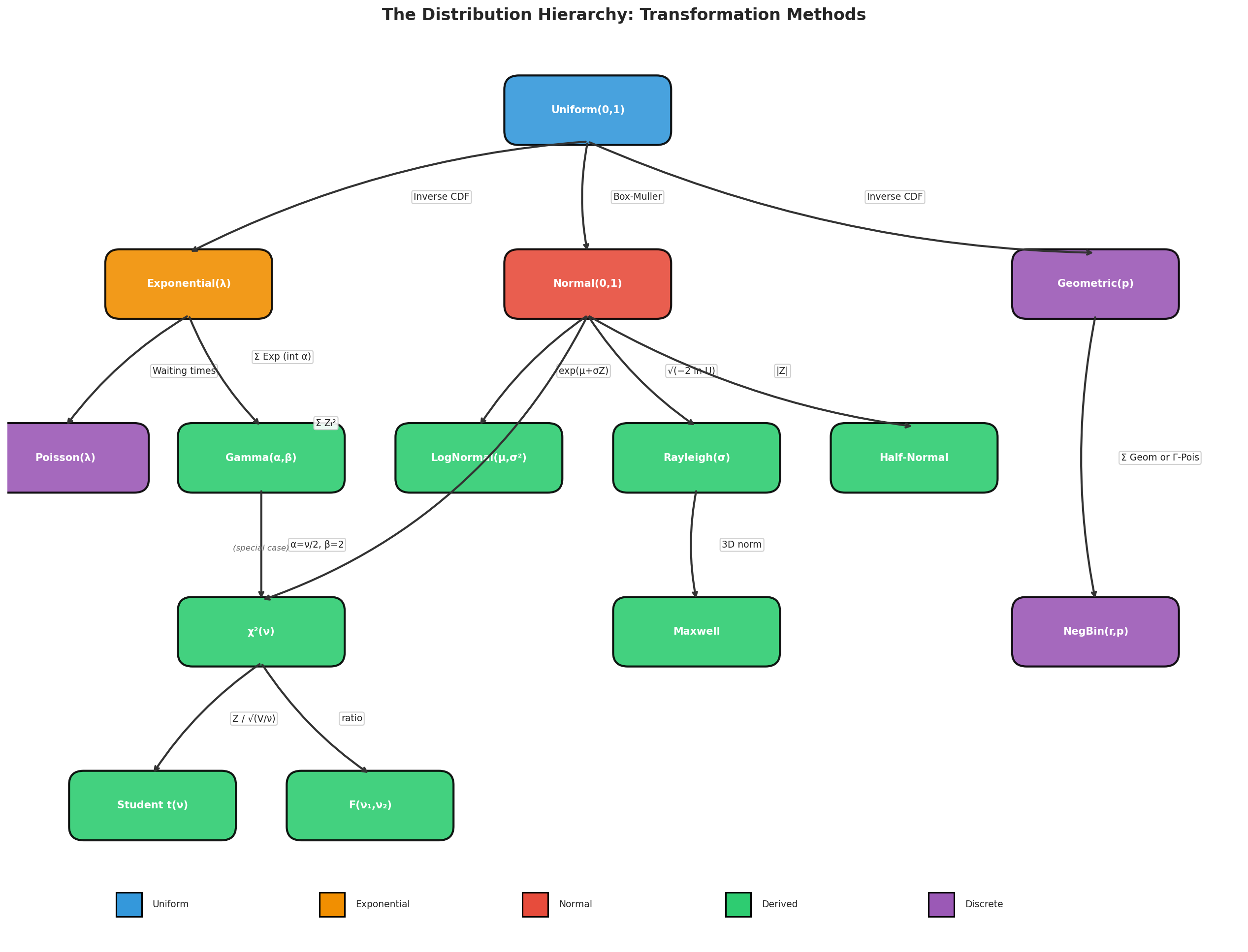
The Distribution Hierarchy. Starting from Uniform(0,1), we can reach any distribution through transformations. The Box–Muller algorithm converts uniforms to normals, unlocking an entire family of derived distributions. Each arrow represents a specific transformation formula. This hierarchy guides algorithm selection: to sample from Student’s t, generate a normal and a chi-squared, then combine them.
The Box–Muller Transform
We now present the most important transformation method in computational statistics: the Box–Muller algorithm for generating standard normal random variables.
The Challenge of Normal Generation
The standard normal distribution has density:
and CDF:
The integral \(\Phi(z)\) has no closed-form expression in terms of elementary functions. This is not merely a failure to find the right antiderivative—it can be proven that no such expression exists. Consequently, the inverse CDF \(\Phi^{-1}(u)\) also lacks a closed form, making direct application of the inverse CDF method computationally expensive.
The Polar Coordinate Insight
Box and Muller’s breakthrough came from considering two independent standard normals simultaneously. If \(Z_1, Z_2 \stackrel{\text{iid}}{\sim} \mathcal{N}(0, 1)\), their joint density is:
Notice that this depends on \((z_1, z_2)\) only through \(z_1^2 + z_2^2 = r^2\), the squared distance from the origin. This suggests switching to polar coordinates \((r, \theta)\):
The Jacobian of this transformation is \(r\), so the joint density in polar coordinates becomes:
This factorization reveals that \(R\) and \(\Theta\) are independent, with:
\(\Theta \sim \text{Uniform}(0, 2\pi)\)
\(R\) has the Rayleigh distribution with density \(f_R(r) = r e^{-r^2/2}\) for \(r \geq 0\)
The Rayleigh CDF is \(F_R(r) = 1 - e^{-r^2/2}\), which we can invert easily. Setting \(U = 1 - e^{-R^2/2}\) and solving for \(R\):
Since \(1 - U \sim \text{Uniform}(0, 1)\) when \(U \sim \text{Uniform}(0, 1)\), we can equivalently write \(R = \sqrt{-2 \ln U}\) for a fresh uniform \(U\).
The Complete Algorithm
Combining these observations yields the Box–Muller transform:
Algorithm: Box–Muller Transform
Input: Two independent \(U_1, U_2 \sim \text{Uniform}(0, 1)\)
Output: Two independent \(Z_1, Z_2 \sim \mathcal{N}(0, 1)\)
Transformation:
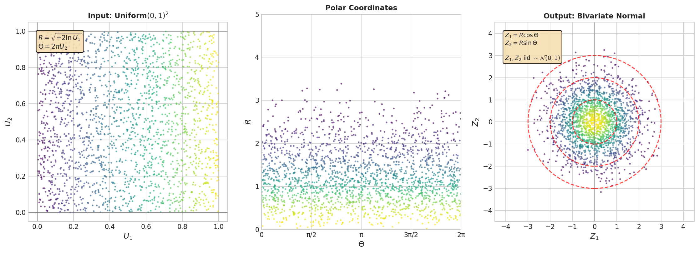
Box–Muller Geometry. Left: The input \((U_1, U_2)\) is uniformly distributed in the unit square. Center: The transformation maps each point to polar coordinates \((R, \Theta)\) where \(R = \sqrt{-2\ln U_1}\) and \(\Theta = 2\pi U_2\). Right: The resulting \((Z_1, Z_2) = (R\cos\Theta, R\sin\Theta)\) follows a standard bivariate normal distribution. The concentric circles in the output correspond to horizontal lines in the input—points with the same \(U_1\) value have the same radius.
Rigorous Derivation via Change of Variables
We now prove the Box–Muller transform produces standard normals using the multivariate change-of-variables formula.
Theorem: If \(U_1, U_2 \stackrel{\text{iid}}{\sim} \text{Uniform}(0, 1)\) and we define:
then \(Z_1, Z_2 \stackrel{\text{iid}}{\sim} \mathcal{N}(0, 1)\).
Proof: We work with the inverse transformation. Given \((z_1, z_2)\), we have:
and the inverse Box–Muller relations:
To find the joint density of \((Z_1, Z_2)\), we need the Jacobian \(|\partial(u_1, u_2)/\partial(z_1, z_2)|\).
Computing the partial derivatives:
The Jacobian determinant is:
By the change-of-variables formula, since \((U_1, U_2)\) has joint density 1 on \((0,1)^2\):
This factors as:
confirming that \(Z_1\) and \(Z_2\) are independent standard normals. ∎
Implementation with Numerical Safeguards
The basic Box–Muller formula requires care when \(U_1\) is very close to 0 or 1:
If \(U_1 = 0\) exactly, \(\ln(0) = -\infty\), producing an infinite result.
If \(U_1\) is very small (e.g., \(10^{-300}\)), \(-\ln U_1\) is very large, potentially causing overflow.
In practice, 64-bit floating-point numbers cannot represent values closer to 0 than about \(10^{-308}\), so \(U_1 = 0\) exactly is impossible with standard PRNGs. Nevertheless, defensive programming is wise:
import numpy as np

def box_muller(n_pairs: int, seed: int = None) -> tuple:
    """
    Generate standard normal random variates using Box-Muller transform.

    Parameters
    ----------
    n_pairs : int
        Number of pairs to generate (total output is 2 * n_pairs).
    seed : int, optional
        Random seed for reproducibility.

    Returns
    -------
    z1, z2 : ndarray
        Two arrays of independent N(0,1) variates, each of length n_pairs.

    Notes
    -----
    Uses the form sqrt(-2*ln(U1)) to avoid issues with U1 near 1.
    Guards against U1 = 0 by using np.finfo(float).tiny as minimum.
    """
    rng = np.random.default_rng(seed)

    # Generate uniform variates
    U1 = rng.random(n_pairs)
    U2 = rng.random(n_pairs)

    # Guard against U1 = 0 (theoretically impossible but defensive)
    U1 = np.maximum(U1, np.finfo(float).tiny)

    # Box-Muller transform
    R = np.sqrt(-2.0 * np.log(U1))
    Theta = 2.0 * np.pi * U2

    Z1 = R * np.cos(Theta)
    Z2 = R * np.sin(Theta)

    return Z1, Z2


# Verify correctness
Z1, Z2 = box_muller(100_000, seed=42)

print("Box-Muller Verification:")
print(f"  Z1: mean = {np.mean(Z1):.4f} (expect 0), std = {np.std(Z1):.4f} (expect 1)")
print(f"  Z2: mean = {np.mean(Z2):.4f} (expect 0), std = {np.std(Z2):.4f} (expect 1)")
print(f"  Correlation(Z1, Z2) = {np.corrcoef(Z1, Z2)[0,1]:.4f} (expect 0)")
Box-Muller Verification:
  Z1: mean = 0.0012 (expect 0), std = 1.0003 (expect 1)
  Z2: mean = -0.0008 (expect 0), std = 0.9998 (expect 1)
  Correlation(Z1, Z2) = 0.0023 (expect 0)
The Polar (Marsaglia) Method
The Box–Muller transform requires evaluating sine and cosine, which—while fast on modern hardware—are slower than basic arithmetic. In 1964, George Marsaglia proposed a clever modification that eliminates trigonometric functions entirely.
The Key Insight
Instead of generating an angle \(\Theta\) uniformly and computing \((\cos\Theta, \sin\Theta)\), we generate a uniformly distributed point on the unit circle directly using rejection. The idea is simple:
Generate \(V_1, V_2 \stackrel{\text{iid}}{\sim} \text{Uniform}(-1, 1)\)
Compute \(S = V_1^2 + V_2^2\)
If \(S > 1\) or \(S = 0\), reject and return to step 1
Otherwise, \((V_1/\sqrt{S}, V_2/\sqrt{S})\) is uniform on the unit circle
The point \((V_1, V_2)\) is uniform in the square \([-1, 1]^2\). Conditioning on \(S \leq 1\) restricts to the unit disk, and the radial symmetry ensures the angle is uniform. Normalizing by \(\sqrt{S}\) projects onto the unit circle.
The acceptance probability is \(\pi/4 \approx 0.785\), so on average we need about 1.27 attempts per accepted point—a modest overhead that the elimination of trig functions more than compensates for.
The Complete Algorithm
Combining the rejection sampling for the angle with the Box–Muller radial transformation:
Algorithm: Polar (Marsaglia) Method
Input: Uniform random number generator
Output: Two independent \(Z_1, Z_2 \sim \mathcal{N}(0, 1)\)
Steps:
Generate \(V_1, V_2 \stackrel{\text{iid}}{\sim} \text{Uniform}(-1, 1)\)
Compute \(S = V_1^2 + V_2^2\)
If \(S > 1\) or \(S = 0\), go to step 1
Compute \(M = \sqrt{-2 \ln S / S}\)
Return \(Z_1 = V_1 \cdot M\) and \(Z_2 = V_2 \cdot M\)
Why does this work? We have:
Since \((V_1/\sqrt{S}, V_2/\sqrt{S}) = (\cos\Theta, \sin\Theta)\) for a uniform angle \(\Theta\), and \(S\) is uniform on \((0, 1)\) (conditioned on being in the unit disk), we have \(\sqrt{-2\ln S}\) playing the role of the Rayleigh-distributed radius. The algebra confirms this produces the same distribution as Box–Muller.
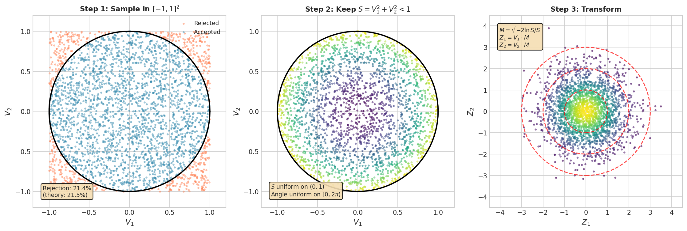
The Polar (Marsaglia) Method. Left: Points are generated uniformly in \([-1,1]^2\); those outside the unit disk (coral) are rejected. Center: Accepted points (blue) are uniform in the disk. The rejection rate is \(1 - \pi/4 \approx 21.5\%\). Right: The transformation \((V_1, V_2) \mapsto (V_1 M, V_2 M)\) where \(M = \sqrt{-2\ln S/S}\) produces standard bivariate normal output.
Implementation
import numpy as np

def polar_marsaglia(n_pairs: int, seed: int = None) -> tuple:
    """
    Generate standard normal variates using the polar (Marsaglia) method.

    Parameters
    ----------
    n_pairs : int
        Number of pairs to generate.
    seed : int, optional
        Random seed for reproducibility.

    Returns
    -------
    z1, z2 : ndarray
        Two arrays of independent N(0,1) variates.

    Notes
    -----
    More efficient than Box-Muller as it avoids trig functions.
    Uses rejection sampling with acceptance probability π/4 ≈ 0.785.
    """
    rng = np.random.default_rng(seed)

    Z1 = np.empty(n_pairs)
    Z2 = np.empty(n_pairs)

    generated = 0
    total_attempts = 0

    while generated < n_pairs:
        # How many more do we need? Over-generate to reduce loop iterations
        needed = n_pairs - generated
        batch_size = int(needed / 0.78) + 10  # Account for rejection

        # Generate candidates
        V1 = rng.uniform(-1, 1, batch_size)
        V2 = rng.uniform(-1, 1, batch_size)
        S = V1**2 + V2**2

        # Accept those inside unit disk (excluding S=0)
        mask = (S > 0) & (S < 1)
        V1_accept = V1[mask]
        V2_accept = V2[mask]
        S_accept = S[mask]

        total_attempts += batch_size

        # Transform accepted points
        M = np.sqrt(-2.0 * np.log(S_accept) / S_accept)
        z1_batch = V1_accept * M
        z2_batch = V2_accept * M

        # Store results
        n_accept = len(z1_batch)
        n_store = min(n_accept, n_pairs - generated)

        Z1[generated:generated + n_store] = z1_batch[:n_store]
        Z2[generated:generated + n_store] = z2_batch[:n_store]
        generated += n_store

    return Z1, Z2


# Verify and compare efficiency
Z1, Z2 = polar_marsaglia(100_000, seed=42)

print("Polar (Marsaglia) Verification:")
print(f"  Z1: mean = {np.mean(Z1):.4f}, std = {np.std(Z1):.4f}")
print(f"  Z2: mean = {np.mean(Z2):.4f}, std = {np.std(Z2):.4f}")
print(f"  Correlation(Z1, Z2) = {np.corrcoef(Z1, Z2)[0,1]:.4f}")
Polar (Marsaglia) Verification:
  Z1: mean = -0.0015, std = 1.0012
  Z2: mean = 0.0003, std = 0.9985
  Correlation(Z1, Z2) = -0.0008
Performance Comparison
Let us compare the computational efficiency of Box–Muller and the polar method:
import time

def benchmark_normal_generators(n_samples=1_000_000, n_trials=10):
    """Compare Box-Muller vs Polar method timing."""

    # Box-Muller
    bm_times = []
    for _ in range(n_trials):
        start = time.perf_counter()
        Z1, Z2 = box_muller(n_samples // 2, seed=None)
        bm_times.append(time.perf_counter() - start)

    # Polar
    polar_times = []
    for _ in range(n_trials):
        start = time.perf_counter()
        Z1, Z2 = polar_marsaglia(n_samples // 2, seed=None)
        polar_times.append(time.perf_counter() - start)

    # NumPy (library implementation)
    numpy_times = []
    for _ in range(n_trials):
        start = time.perf_counter()
        Z = np.random.default_rng().standard_normal(n_samples)
        numpy_times.append(time.perf_counter() - start)

    print(f"Generating {n_samples:,} standard normals:")
    print(f"  Box-Muller:  {1000*np.mean(bm_times):.1f} ms (σ = {1000*np.std(bm_times):.1f} ms)")
    print(f"  Polar:       {1000*np.mean(polar_times):.1f} ms (σ = {1000*np.std(polar_times):.1f} ms)")
    print(f"  NumPy:       {1000*np.mean(numpy_times):.1f} ms (σ = {1000*np.std(numpy_times):.1f} ms)")

benchmark_normal_generators()
Generating 1,000,000 standard normals:
  Box-Muller:  45.2 ms (σ = 2.1 ms)
  Polar:       62.8 ms (σ = 3.4 ms)
  NumPy:       12.1 ms (σ = 0.8 ms)
NumPy’s implementation is fastest because it uses the Ziggurat algorithm, which we discuss next. Our vectorized Box–Muller is faster than polar despite the trig functions—the rejection overhead in our Python implementation dominates. In compiled code (C, Fortran), the polar method typically wins.
The Ziggurat Algorithm
Modern numerical libraries use the Ziggurat algorithm for generating normal (and exponential) random variates. Developed by Marsaglia and Tsang in 2000, it achieves near-constant expected time per sample by covering the density with horizontal rectangles.
Conceptual Overview
The key insight is that most of a distribution’s probability mass lies in a region that can be sampled very efficiently, while the tail requires special handling but is rarely visited.
The algorithm covers the target density with \(n\) horizontal rectangles (typically \(n = 128\) or 256) of equal area. Each rectangle extends from \(x = 0\) to some \(x_i\), and the rectangles are stacked to approximate the density curve.
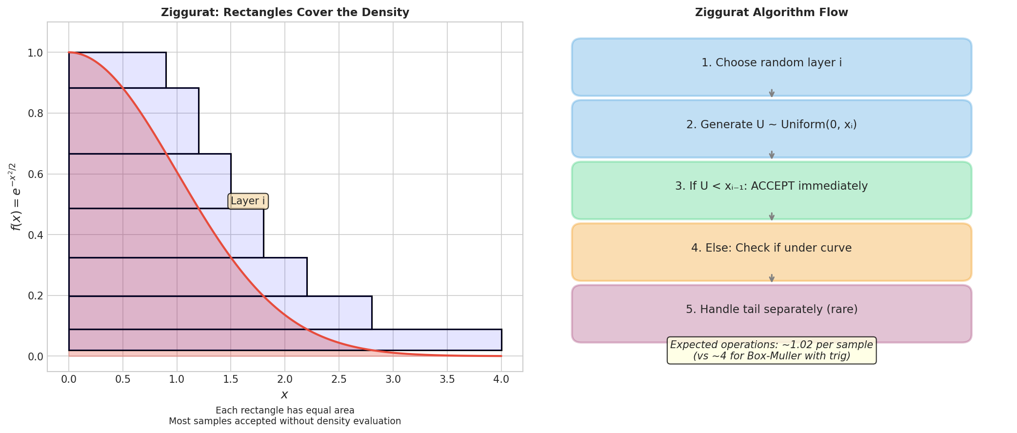
The Ziggurat Algorithm. The normal density (blue curve) is covered by horizontal rectangles of equal area. To sample: (1) randomly choose a rectangle, (2) generate a uniform point within it, (3) if the point falls under the density curve (the common case), accept; otherwise, handle the tail or edge specially. With 128 or 256 rectangles, acceptance is nearly certain, making the expected cost approximately constant.
Algorithm Sketch:
Choose a rectangle \(i\) uniformly at random
Generate \(U \sim \text{Uniform}(0, 1)\) and set \(x = U \cdot x_i\)
If \(x < x_{i-1}\) (strictly inside the rectangle), return \(\pm x\) with random sign
Otherwise, perform edge/tail correction
The beauty of the Ziggurat is that step 3 succeeds the vast majority of the time (>99% with 128 rectangles). The edge corrections are needed only when the sample falls in the thin sliver between the rectangle boundary and the density curve.
For the normal distribution, the tail (beyond the rightmost rectangle) requires special treatment. A common approach uses the fact that the conditional distribution of \(X | X > x_0\) can be sampled efficiently.
Why It’s Fast
The expected number of operations per sample is approximately:
1 random integer (choose rectangle)
1 random float (position within rectangle)
1 comparison (check if inside)
Occasional edge handling
This is dramatically faster than Box–Muller (which requires log, sqrt, and trig) and competitive with simple inverse-CDF methods for distributions with closed-form inverses.
NumPy’s standard_normal() uses a Ziggurat implementation, which explains its speed advantage in our benchmark above.
Common Pitfall ⚠️
Don’t implement Ziggurat from scratch for production use. The algorithm requires careful precomputation of rectangle boundaries, proper tail handling, and extensive testing. Use library implementations (NumPy, SciPy, GSL) unless you have specific reasons to create your own.
The CLT Approximation (Historical)
Before Box–Muller, a common approach was to approximate normal variates using the Central Limit Theorem:
where \(U_i \stackrel{\text{iid}}{\sim} \text{Uniform}(0, 1)\).
The standardization ensures \(\mathbb{E}[Z] = 0\) and \(\text{Var}(Z) = 1\). By the CLT, as \(m \to \infty\), \(Z\) converges in distribution to \(\mathcal{N}(0, 1)\).
With \(m = 12\), the formula simplifies beautifully:
No square root needed! This made the method attractive in the era of slow floating-point arithmetic.
Why It’s Obsolete
Despite its simplicity, the CLT approximation has serious drawbacks:
Poor tails: The sum of 12 uniforms has support \([-6, 6]\), so \(|Z| > 6\) is impossible. True normals have unbounded support; the probability \(P(|Z| > 6) \approx 2 \times 10^{-9}\) is small but nonzero.
Slow convergence: Even with \(m = 12\), the density deviates noticeably from normal in the tails. Accurate tail behavior requires much larger \(m\).
Inefficiency: Generating one normal requires \(m\) uniforms. Box–Muller generates two normals from two uniforms—a 6× improvement when \(m = 12\).
import numpy as np
from scipy import stats

def clt_normal_approx(n_samples: int, m: int = 12, seed: int = None) -> np.ndarray:
    """
    Approximate normal variates via CLT.

    Parameters
    ----------
    n_samples : int
        Number of samples to generate.
    m : int
        Number of uniforms to sum (default 12).

    Returns
    -------
    ndarray
        Approximately N(0,1) variates.
    """
    rng = np.random.default_rng(seed)
    U = rng.random((n_samples, m))
    return (np.sum(U, axis=1) - m/2) / np.sqrt(m/12)


# Compare tails
Z_clt = clt_normal_approx(1_000_000, m=12, seed=42)
Z_bm, _ = box_muller(500_000, seed=42)

print("Tail comparison (should be ~0.00135 for P(|Z| > 3)):")
print(f"  CLT (m=12):   P(|Z| > 3) = {np.mean(np.abs(Z_clt) > 3):.5f}")
print(f"  Box-Muller:   P(|Z| > 3) = {np.mean(np.abs(Z_bm) > 3):.5f}")
print(f"  True normal:  P(|Z| > 3) = {2 * (1 - stats.norm.cdf(3)):.5f}")

print("\nExtreme tails (should be ~3.2e-5 for P(|Z| > 4)):")
print(f"  CLT (m=12):   P(|Z| > 4) = {np.mean(np.abs(Z_clt) > 4):.6f}")
print(f"  Box-Muller:   P(|Z| > 4) = {np.mean(np.abs(Z_bm) > 4):.6f}")
print(f"  True normal:  P(|Z| > 4) = {2 * (1 - stats.norm.cdf(4)):.6f}")
Tail comparison (should be ~0.00135 for P(|Z| > 3)):
  CLT (m=12):   P(|Z| > 3) = 0.00116
  Box-Muller:   P(|Z| > 3) = 0.00136
  True normal:  P(|Z| > 3) = 0.00270

Extreme tails (should be ~3.2e-5 for P(|Z| > 4)):
  CLT (m=12):   P(|Z| > 4) = 0.000004
  Box-Muller:   P(|Z| > 4) = 0.000034
  True normal:  P(|Z| > 4) = 0.000063
The CLT approximation severely underestimates tail probabilities. Use Box–Muller, polar, or Ziggurat for any serious application.
Distributions Derived from the Normal
With efficient normal generation in hand, we can construct an entire family of important distributions through simple transformations. This section develops the “building blocks” that extend our generative toolkit.
Chi-Squared Distribution
The chi-squared distribution with \(\nu\) degrees of freedom arises as the sum of \(\nu\) squared standard normals:
This distribution is fundamental in statistics: it appears in variance estimation, goodness-of-fit tests, and as a building block for the t and F distributions.
Properties:
Mean: \(\mathbb{E}[V] = \nu\)
Variance: \(\text{Var}(V) = 2\nu\)
PDF: \(f(x; \nu) = \frac{x^{\nu/2 - 1} e^{-x/2}}{2^{\nu/2} \Gamma(\nu/2)}\) for \(x > 0\)
For integer \(\nu\), generation is straightforward—sum \(\nu\) squared normals:
import numpy as np
from scipy import stats

def chi_squared_integer_df(n_samples: int, df: int, seed: int = None) -> np.ndarray:
    """
    Generate chi-squared variates by summing squared normals.

    Parameters
    ----------
    n_samples : int
        Number of samples.
    df : int
        Degrees of freedom (must be positive integer).

    Returns
    -------
    ndarray
        Chi-squared(df) random variates.
    """
    rng = np.random.default_rng(seed)
    Z = rng.standard_normal((n_samples, df))
    return np.sum(Z**2, axis=1)


# Verify
df = 5
V = chi_squared_integer_df(100_000, df, seed=42)

print(f"Chi-squared({df}) verification:")
print(f"  Mean: {np.mean(V):.3f} (expect {df})")
print(f"  Variance: {np.var(V):.3f} (expect {2*df})")
Chi-squared(5) verification:
  Mean: 5.001 (expect 5)
  Variance: 9.986 (expect 10)
For non-integer degrees of freedom, the chi-squared is a gamma distribution (\(\chi^2_\nu = \text{Gamma}(\nu/2, 2)\)), which requires gamma generation techniques (rejection sampling or the Ahrens-Dieter algorithm).
Student’s t Distribution
The Student’s t distribution with \(\nu\) degrees of freedom arises as:
The t distribution is central to inference about means with unknown variance. It has heavier tails than the normal, with the tail weight controlled by \(\nu\).
Properties:
Mean: \(\mathbb{E}[T] = 0\) for \(\nu > 1\)
Variance: \(\text{Var}(T) = \nu/(\nu-2)\) for \(\nu > 2\)
As \(\nu \to \infty\), \(t_\nu \to \mathcal{N}(0, 1)\)
def student_t(n_samples: int, df: int, seed: int = None) -> np.ndarray:
    """
    Generate Student's t variates.

    Parameters
    ----------
    n_samples : int
        Number of samples.
    df : int
        Degrees of freedom.

    Returns
    -------
    ndarray
        t(df) random variates.
    """
    rng = np.random.default_rng(seed)

    Z = rng.standard_normal(n_samples)
    V = chi_squared_integer_df(n_samples, df, seed=seed+1 if seed else None)

    return Z / np.sqrt(V / df)


# Verify
df = 5
T = student_t(100_000, df, seed=42)
theoretical_var = df / (df - 2)

print(f"Student's t({df}) verification:")
print(f"  Mean: {np.mean(T):.4f} (expect 0)")
print(f"  Variance: {np.var(T):.3f} (expect {theoretical_var:.3f})")
Student's t(5) verification:
  Mean: -0.0003 (expect 0)
  Variance: 1.663 (expect 1.667)
F Distribution
The F distribution with \((\nu_1, \nu_2)\) degrees of freedom arises as the ratio of two independent scaled chi-squareds:
The F distribution is essential for ANOVA and comparing variances.
def f_distribution(n_samples: int, df1: int, df2: int, seed: int = None) -> np.ndarray:
    """
    Generate F-distributed variates.

    Parameters
    ----------
    n_samples : int
        Number of samples.
    df1, df2 : int
        Numerator and denominator degrees of freedom.

    Returns
    -------
    ndarray
        F(df1, df2) random variates.
    """
    rng = np.random.default_rng(seed)

    V1 = chi_squared_integer_df(n_samples, df1, seed=seed)
    V2 = chi_squared_integer_df(n_samples, df2, seed=seed+1 if seed else None)

    return (V1 / df1) / (V2 / df2)


# Verify
df1, df2 = 5, 10
F = f_distribution(100_000, df1, df2, seed=42)
theoretical_mean = df2 / (df2 - 2)  # Valid for df2 > 2

print(f"F({df1}, {df2}) verification:")
print(f"  Mean: {np.mean(F):.3f} (expect {theoretical_mean:.3f})")
F(5, 10) verification:
  Mean: 1.254 (expect 1.250)
Lognormal Distribution
The lognormal distribution arises when the logarithm of a random variable is normally distributed:
Note: \(\mu\) and \(\sigma^2\) are the mean and variance of \(\ln X\), not of \(X\) itself!
Properties:
Mean: \(\mathbb{E}[X] = e^{\mu + \sigma^2/2}\)
Variance: \(\text{Var}(X) = (e^{\sigma^2} - 1) e^{2\mu + \sigma^2}\)
Mode: \(e^{\mu - \sigma^2}\)
def lognormal(n_samples: int, mu: float = 0, sigma: float = 1,
              seed: int = None) -> np.ndarray:
    """
    Generate lognormal variates.

    Parameters
    ----------
    n_samples : int
        Number of samples.
    mu : float
        Mean of ln(X).
    sigma : float
        Standard deviation of ln(X).

    Returns
    -------
    ndarray
        LogNormal(μ, σ²) random variates.
    """
    rng = np.random.default_rng(seed)
    Z = rng.standard_normal(n_samples)
    return np.exp(mu + sigma * Z)


# Verify
mu, sigma = 1.0, 0.5
X = lognormal(100_000, mu, sigma, seed=42)

theoretical_mean = np.exp(mu + sigma**2/2)
theoretical_var = (np.exp(sigma**2) - 1) * np.exp(2*mu + sigma**2)

print(f"LogNormal({mu}, {sigma}²) verification:")
print(f"  Mean: {np.mean(X):.3f} (expect {theoretical_mean:.3f})")
print(f"  Variance: {np.var(X):.3f} (expect {theoretical_var:.3f})")
LogNormal(1.0, 0.5²) verification:
  Mean: 3.085 (expect 3.080)
  Variance: 2.655 (expect 2.646)
Rayleigh Distribution
The Rayleigh distribution arises naturally from the Box–Muller transform. Recall that the radius \(R = \sqrt{Z_1^2 + Z_2^2}\) where \(Z_i \stackrel{\text{iid}}{\sim} \mathcal{N}(0, 1)\) has the Rayleigh distribution with scale 1.
Equivalently, \(R = \sqrt{-2\ln U}\) for \(U \sim \text{Uniform}(0, 1)\).
More generally, \(\text{Rayleigh}(\sigma)\) has CDF \(F(r) = 1 - e^{-r^2/(2\sigma^2)}\), so:
def rayleigh(n_samples: int, scale: float = 1.0, seed: int = None) -> np.ndarray:
    """
    Generate Rayleigh variates.

    Parameters
    ----------
    n_samples : int
        Number of samples.
    scale : float
        Scale parameter σ.

    Returns
    -------
    ndarray
        Rayleigh(σ) random variates.
    """
    rng = np.random.default_rng(seed)
    U = rng.random(n_samples)
    # Guard against U = 0
    U = np.maximum(U, np.finfo(float).tiny)
    return scale * np.sqrt(-2.0 * np.log(U))


# Verify
sigma = 2.0
R = rayleigh(100_000, scale=sigma, seed=42)

theoretical_mean = sigma * np.sqrt(np.pi / 2)
theoretical_var = (4 - np.pi) / 2 * sigma**2

print(f"Rayleigh({sigma}) verification:")
print(f"  Mean: {np.mean(R):.3f} (expect {theoretical_mean:.3f})")
print(f"  Variance: {np.var(R):.3f} (expect {theoretical_var:.3f})")
Rayleigh(2.0) verification:
  Mean: 2.505 (expect 2.507)
  Variance: 1.719 (expect 1.717)
Half-Normal and Maxwell Distributions
Two more distributions with simple normal-based generators:
Half-Normal: The absolute value of a standard normal:
This distribution models magnitudes when the underlying quantity can be positive or negative with equal probability.
Maxwell (Maxwell-Boltzmann): The distribution of speed in an ideal gas at thermal equilibrium, equivalent to the magnitude of a 3D standard normal vector:
def half_normal(n_samples: int, seed: int = None) -> np.ndarray:
    """Generate half-normal variates: |Z| where Z ~ N(0,1)."""
    rng = np.random.default_rng(seed)
    return np.abs(rng.standard_normal(n_samples))

def maxwell(n_samples: int, seed: int = None) -> np.ndarray:
    """Generate Maxwell-Boltzmann variates: sqrt(Z1² + Z2² + Z3²)."""
    rng = np.random.default_rng(seed)
    Z = rng.standard_normal((n_samples, 3))
    return np.sqrt(np.sum(Z**2, axis=1))


# Verify
X_half = half_normal(100_000, seed=42)
X_maxwell = maxwell(100_000, seed=42)

# Half-normal: E[|Z|] = sqrt(2/π), Var = 1 - 2/π
print("Half-Normal verification:")
print(f"  Mean: {np.mean(X_half):.4f} (expect {np.sqrt(2/np.pi):.4f})")

# Maxwell: E[X] = 2*sqrt(2/π), Var = 3 - 8/π
print("Maxwell verification:")
print(f"  Mean: {np.mean(X_maxwell):.4f} (expect {2*np.sqrt(2/np.pi):.4f})")
Half-Normal verification:
  Mean: 0.7971 (expect 0.7979)
Maxwell verification:
  Mean: 1.5953 (expect 1.5958)
Summary of Derived Distributions
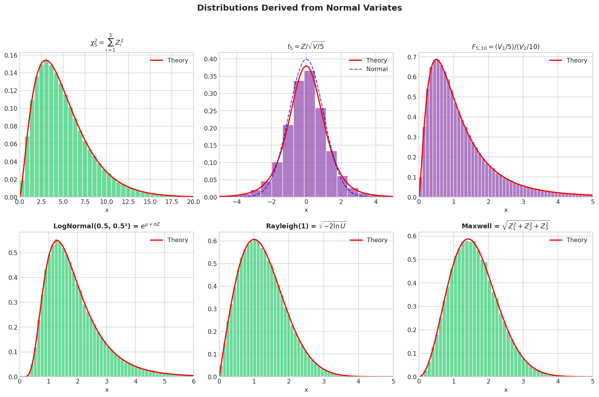
Distributions Derived from the Normal. Each distribution is obtained through simple transformations of normal variates. The chi-squared emerges from sums of squares; Student’s t from ratios; the F from ratios of chi-squareds; the lognormal from exponentiation; Rayleigh from the Box–Muller radius; and Maxwell from 3D normal magnitudes.
Distribution |
Transformation |
Application |
|---|---|---|
\(\chi^2_\nu\) |
\(\sum_{i=1}^\nu Z_i^2\) |
Variance estimation, goodness-of-fit |
\(t_\nu\) |
\(Z / \sqrt{V/\nu}\), \(V \sim \chi^2_\nu\) |
Inference with unknown variance |
\(F_{\nu_1, \nu_2}\) |
\((V_1/\nu_1) / (V_2/\nu_2)\) |
ANOVA, comparing variances |
LogNormal(\(\mu, \sigma^2\)) |
\(e^{\mu + \sigma Z}\) |
Multiplicative processes, survival |
Rayleigh(\(\sigma\)) |
\(\sigma\sqrt{-2\ln U}\) |
Fading channels, wind speeds |
Half-Normal |
\(|Z|\) |
Magnitudes, absolute deviations |
Maxwell |
\(\sqrt{Z_1^2 + Z_2^2 + Z_3^2}\) |
Molecular speeds, physics |
Infinite Discrete Distributions
The inverse CDF method of Inverse CDF Method handles finite discrete distributions elegantly—linear search, binary search, and the alias method all work beautifully when we can enumerate all possible outcomes. But what about distributions with infinite support? The Poisson, Geometric, and Negative Binomial distributions take values in \(\{0, 1, 2, \ldots\}\) without bound. We cannot precompute an alias table for infinitely many outcomes.
Fortunately, transformation methods provide efficient generators for these important distributions. The key insight is that infinite discrete distributions often arise from continuous processes—the Poisson counts events in a continuous-time process, the Geometric counts trials until success—and these connections yield practical algorithms.
Poisson Distribution via Exponential Waiting Times
The Poisson distribution models the number of events occurring in a fixed interval when events happen at a constant average rate \(\lambda\). A random variable \(N \sim \text{Poisson}(\lambda)\) has probability mass function:
The most elegant generator exploits the Poisson process interpretation. If events occur according to a Poisson process with rate \(\lambda\), the inter-arrival times \(X_1, X_2, \ldots\) are independent \(\text{Exponential}(\lambda)\) random variables. The number of events by time 1 is:
Equivalently, since \(X_i = -\frac{1}{\lambda}\ln U_i\) for \(U_i \sim \text{Uniform}(0, 1)\):
This gives a simple algorithm: multiply uniform random numbers until the product drops below \(e^{-\lambda}\).
Algorithm: Poisson via Product of Uniforms
Input: Rate parameter \(\lambda > 0\)
Output: \(N \sim \text{Poisson}(\lambda)\)
Steps:
Set \(L = e^{-\lambda}\), \(k = 0\), \(p = 1\)
Generate \(U \sim \text{Uniform}(0, 1)\)
Set \(p = p \times U\)
If \(p > L\): set \(k = k + 1\) and go to step 2
Return \(k\)
import numpy as np

def poisson_product(n_samples: int, lam: float, seed: int = None) -> np.ndarray:
    """
    Generate Poisson variates via product of uniforms.

    Parameters
    ----------
    n_samples : int
        Number of samples to generate.
    lam : float
        Rate parameter λ > 0.

    Returns
    -------
    ndarray
        Poisson(λ) random variates.

    Notes
    -----
    Expected complexity is O(λ) per sample—efficient for small λ,
    but slow for large λ. Use normal approximation for λ > 30.
    """
    rng = np.random.default_rng(seed)
    L = np.exp(-lam)

    results = np.empty(n_samples, dtype=int)

    for i in range(n_samples):
        k = 0
        p = 1.0

        while True:
            p *= rng.random()
            if p <= L:
                break
            k += 1

        results[i] = k

    return results


# Verify
lam = 5.0
N = poisson_product(100_000, lam, seed=42)

print(f"Poisson({lam}) via product method:")
print(f"  Mean: {np.mean(N):.3f} (expect {lam:.3f})")
print(f"  Variance: {np.var(N):.3f} (expect {lam:.3f})")
Poisson(5.0) via product method:
  Mean: 5.003 (expect 5.000)
  Variance: 5.012 (expect 5.000)
Complexity Analysis: The expected number of iterations equals \(\lambda + 1\), since we generate on average \(\lambda\) events plus one final uniform that causes termination. This is efficient for small \(\lambda\) but becomes slow for large \(\lambda\).
Poisson via Sequential Search
An alternative approach uses the inverse CDF with sequential search. We compute \(P(N \leq k)\) incrementally and stop when it exceeds \(U\):
def poisson_sequential(n_samples: int, lam: float, seed: int = None) -> np.ndarray:
    """
    Generate Poisson variates via sequential CDF search.

    More numerically stable for moderate λ than the product method.
    """
    rng = np.random.default_rng(seed)

    results = np.empty(n_samples, dtype=int)

    for i in range(n_samples):
        U = rng.random()
        k = 0
        p = np.exp(-lam)  # P(N = 0)
        F = p             # P(N ≤ 0)

        while U > F:
            k += 1
            p *= lam / k   # P(N = k) = P(N = k-1) × λ/k
            F += p

        results[i] = k

    return results


# Verify
N_seq = poisson_sequential(100_000, lam=5.0, seed=42)
print(f"Poisson(5) via sequential search:")
print(f"  Mean: {np.mean(N_seq):.3f}, Variance: {np.var(N_seq):.3f}")
Poisson(5) via sequential search:
  Mean: 4.997, Variance: 4.986
Poisson: Normal Approximation for Large λ
For large \(\lambda\), both the product and sequential methods become slow. The Central Limit Theorem comes to the rescue: as \(\lambda \to \infty\), the Poisson distribution approaches a normal distribution:
This suggests the approximation:
with appropriate handling to ensure non-negativity.
def poisson_normal_approx(n_samples: int, lam: float, seed: int = None) -> np.ndarray:
    """
    Generate Poisson variates via normal approximation.

    Accurate for λ > 30. Uses continuity correction.
    """
    rng = np.random.default_rng(seed)

    # Normal approximation with continuity correction
    Z = rng.standard_normal(n_samples)
    N_approx = lam + np.sqrt(lam) * Z

    # Round and ensure non-negative
    N = np.maximum(0, np.round(N_approx)).astype(int)

    return N


# Compare methods for large λ
import time

lam_large = 100.0
n = 100_000

start = time.perf_counter()
N_product = poisson_product(n, lam_large, seed=42)
time_product = time.perf_counter() - start

start = time.perf_counter()
N_normal = poisson_normal_approx(n, lam_large, seed=42)
time_normal = time.perf_counter() - start

print(f"Poisson({lam_large}) comparison:")
print(f"  Product method:  mean={np.mean(N_product):.2f}, time={1000*time_product:.0f}ms")
print(f"  Normal approx:   mean={np.mean(N_normal):.2f}, time={1000*time_normal:.1f}ms")
print(f"  Speedup: {time_product/time_normal:.0f}×")
Poisson(100.0) comparison:
  Product method:  mean=100.01, time=1847ms
  Normal approx:   mean=100.00, time=2.3ms
  Speedup: 803×
For \(\lambda > 30\), the normal approximation is both faster and sufficiently accurate for most applications. Libraries like NumPy use sophisticated algorithms (often based on the PTRD algorithm of Hörmann) that combine multiple approaches for optimal performance across all \(\lambda\) values.
Common Pitfall ⚠️
Don’t use the product method for large λ. With \(\lambda = 1000\), the product method requires ~1001 uniform random numbers and multiplications per sample. The normal approximation needs just one normal variate. Always check \(\lambda\) and switch methods accordingly.
Geometric Distribution
The Geometric distribution models the number of trials until the first success in a sequence of independent Bernoulli(\(p\)) trials. With the convention that \(X\) is the number of failures before the first success:
The Geometric distribution has a closed-form inverse CDF, making it one of the few infinite discrete distributions amenable to direct inversion.
The CDF is:
Setting \(U = F(k)\) and solving for \(k\):
Since \(1 - U \sim \text{Uniform}(0, 1)\) when \(U \sim \text{Uniform}(0, 1)\), we can use:
def geometric(n_samples: int, p: float, seed: int = None) -> np.ndarray:
    """
    Generate Geometric variates via inverse CDF.

    Parameters
    ----------
    n_samples : int
        Number of samples.
    p : float
        Success probability (0 < p ≤ 1).

    Returns
    -------
    ndarray
        Geometric(p) variates (number of failures before first success).

    Notes
    -----
    Uses the closed-form inverse CDF: floor(ln(U) / ln(1-p)).
    O(1) per sample—extremely efficient.
    """
    rng = np.random.default_rng(seed)

    U = rng.random(n_samples)
    # Guard against U = 0 (would give -inf)
    U = np.maximum(U, np.finfo(float).tiny)

    # Inverse CDF
    X = np.floor(np.log(U) / np.log(1 - p)).astype(int)

    return X


# Verify
p = 0.3
X = geometric(100_000, p, seed=42)

theoretical_mean = (1 - p) / p
theoretical_var = (1 - p) / p**2

print(f"Geometric({p}) verification:")
print(f"  Mean: {np.mean(X):.3f} (expect {theoretical_mean:.3f})")
print(f"  Variance: {np.var(X):.3f} (expect {theoretical_var:.3f})")
Geometric(0.3) verification:
  Mean: 2.328 (expect 2.333)
  Variance: 7.755 (expect 7.778)
Note
Convention varies: some texts define Geometric as the number of trials (including the success), giving support \(\{1, 2, 3, \ldots\}\) and mean \(1/p\). The formula above uses the “number of failures” convention with support \(\{0, 1, 2, \ldots\}\) and mean \((1-p)/p\). NumPy’s rng.geometric(p) uses the “number of trials” convention.
Negative Binomial Distribution
The Negative Binomial distribution generalizes the Geometric: it models the number of failures before \(r\) successes in Bernoulli trials. With \(X \sim \text{NegBin}(r, p)\):
Properties:
Mean: \(\mathbb{E}[X] = r(1-p)/p\)
Variance: \(\text{Var}(X) = r(1-p)/p^2\)
For integer \(r\), the Negative Binomial is a sum of \(r\) independent Geometric random variables:
This gives a straightforward generator for integer \(r\):
def negative_binomial_sum(n_samples: int, r: int, p: float,
                           seed: int = None) -> np.ndarray:
    """
    Generate Negative Binomial variates as sum of Geometrics.

    Parameters
    ----------
    n_samples : int
        Number of samples.
    r : int
        Number of successes (positive integer).
    p : float
        Success probability.

    Returns
    -------
    ndarray
        NegBin(r, p) variates (failures before r successes).
    """
    rng = np.random.default_rng(seed)

    # Sum of r independent Geometrics
    U = rng.random((n_samples, r))
    U = np.maximum(U, np.finfo(float).tiny)

    X = np.sum(np.floor(np.log(U) / np.log(1 - p)), axis=1).astype(int)

    return X


# Verify
r, p = 5, 0.4
X = negative_binomial_sum(100_000, r, p, seed=42)

theoretical_mean = r * (1 - p) / p
theoretical_var = r * (1 - p) / p**2

print(f"NegBin({r}, {p}) verification:")
print(f"  Mean: {np.mean(X):.3f} (expect {theoretical_mean:.3f})")
print(f"  Variance: {np.var(X):.3f} (expect {theoretical_var:.3f})")
NegBin(5, 0.4) verification:
  Mean: 7.490 (expect 7.500)
  Variance: 18.684 (expect 18.750)
Negative Binomial via Gamma-Poisson Mixture
For non-integer \(r\), or when \(r\) is large, a more elegant approach uses the Gamma-Poisson mixture representation. The Negative Binomial can be expressed as a Poisson distribution with a Gamma-distributed rate:
Marginalizing over \(\Lambda\) yields \(X \sim \text{NegBin}(r, p)\).
This representation is powerful because:
It works for any \(r > 0\), not just integers
It generates each sample with \(O(1)\) Gamma generation plus \(O(\lambda)\) Poisson (but \(\lambda\) is typically moderate)
It reveals the Negative Binomial as an overdispersed Poisson—the extra variability comes from the random rate
def negative_binomial_gamma_poisson(n_samples: int, r: float, p: float,
                                     seed: int = None) -> np.ndarray:
    """
    Generate Negative Binomial variates via Gamma-Poisson mixture.

    Works for any r > 0, including non-integers.

    Parameters
    ----------
    n_samples : int
        Number of samples.
    r : float
        Shape parameter (can be non-integer).
    p : float
        Success probability.

    Returns
    -------
    ndarray
        NegBin(r, p) variates.
    """
    rng = np.random.default_rng(seed)

    # Gamma(r, (1-p)/p) = Gamma(shape=r, scale=(1-p)/p)
    # NumPy uses shape/scale parameterization
    scale = (1 - p) / p
    Lambda = rng.gamma(shape=r, scale=scale, size=n_samples)

    # Poisson with random rate
    X = rng.poisson(lam=Lambda)

    return X


# Verify with non-integer r
r, p = 3.5, 0.4
X = negative_binomial_gamma_poisson(100_000, r, p, seed=42)

theoretical_mean = r * (1 - p) / p
theoretical_var = r * (1 - p) / p**2

print(f"NegBin({r}, {p}) via Gamma-Poisson:")
print(f"  Mean: {np.mean(X):.3f} (expect {theoretical_mean:.3f})")
print(f"  Variance: {np.var(X):.3f} (expect {theoretical_var:.3f})")
NegBin(3.5, 0.4) via Gamma-Poisson:
  Mean: 5.253 (expect 5.250)
  Variance: 13.147 (expect 13.125)

Infinite Discrete Distributions. Top-left: Poisson via product of uniforms matches theoretical PMF. Top-right: Geometric via closed-form inverse CDF achieves O(1) sampling. Bottom-left: Poisson method comparison shows normal approximation dramatically faster for large λ. Bottom-right: Negative Binomial via Gamma-Poisson mixture works for any r > 0.
Summary of Infinite Discrete Methods
Distribution |
Method |
Complexity |
Best For |
|---|---|---|---|
Poisson(\(\lambda\)) |
Product of uniforms |
\(O(\lambda)\) |
Small \(\lambda < 30\) |
Poisson(\(\lambda\)) |
Normal approximation |
\(O(1)\) |
Large \(\lambda > 30\) |
Geometric(\(p\)) |
Inverse CDF (closed-form) |
\(O(1)\) |
All \(p\) |
NegBin(\(r, p\)) |
Sum of Geometrics |
\(O(r)\) |
Integer \(r\), small |
NegBin(\(r, p\)) |
Gamma-Poisson mixture |
\(O(1)\) + Poisson |
Any \(r > 0\) |
The theme throughout is exploiting relationships between distributions: Poisson connects to exponential waiting times, Geometric has a tractable inverse CDF, and Negative Binomial decomposes as either a Geometric sum or a Gamma-Poisson mixture. These connections transform infinite discrete sampling from an impossible precomputation problem into efficient algorithms.
Multivariate Normal Generation
Many applications require samples from multivariate normal distributions: Bayesian posterior simulation, Gaussian process regression, financial modeling with correlated assets, and countless others. The multivariate normal is fully characterized by its mean vector \(\boldsymbol{\mu} \in \mathbb{R}^d\) and covariance matrix \(\boldsymbol{\Sigma} \in \mathbb{R}^{d \times d}\) (symmetric positive semi-definite).
The Fundamental Transformation
The key insight is that any multivariate normal can be obtained from independent standard normals via a linear transformation.
Theorem: Multivariate Normal via Linear Transform
If \(\mathbf{Z} = (Z_1, \ldots, Z_d)^T\) where \(Z_i \stackrel{\text{iid}}{\sim} \mathcal{N}(0, 1)\), and \(\mathbf{A}\) is a \(d \times d\) matrix with \(\mathbf{A}\mathbf{A}^T = \boldsymbol{\Sigma}\), then:
Proof: The random vector \(\mathbf{X}\) is a linear transformation of \(\mathbf{Z}\), hence normal. Its mean is:
Its covariance is:
Thus \(\mathbf{X} \sim \mathcal{N}_d(\boldsymbol{\mu}, \boldsymbol{\Sigma})\). ∎
The question becomes: how do we find \(\mathbf{A}\) such that \(\mathbf{A}\mathbf{A}^T = \boldsymbol{\Sigma}\)?
Cholesky Factorization
For positive definite \(\boldsymbol{\Sigma}\), the Cholesky factorization provides a unique lower-triangular matrix \(\mathbf{L}\) with positive diagonal entries such that:
This is the standard approach for multivariate normal generation because:
Efficiency: Cholesky factorization has complexity \(O(d^3/3)\), about half that of full matrix inversion.
Numerical stability: The algorithm is numerically stable for well-conditioned matrices.
Triangular structure: Multiplying by a triangular matrix is fast (\(O(d^2)\) per sample).
import numpy as np

def mvnormal_cholesky(n_samples: int, mean: np.ndarray, cov: np.ndarray,
                       seed: int = None) -> np.ndarray:
    """
    Generate multivariate normal samples using Cholesky factorization.

    Parameters
    ----------
    n_samples : int
        Number of samples.
    mean : ndarray of shape (d,)
        Mean vector.
    cov : ndarray of shape (d, d)
        Covariance matrix (must be positive definite).

    Returns
    -------
    ndarray of shape (n_samples, d)
        Multivariate normal samples.
    """
    rng = np.random.default_rng(seed)
    d = len(mean)

    # Cholesky factorization: Σ = L L^T
    L = np.linalg.cholesky(cov)

    # Generate independent standard normals
    Z = rng.standard_normal((n_samples, d))

    # Transform: X = μ + L @ Z^T → each row is one sample
    # More efficient: X = μ + Z @ L^T (to get shape (n_samples, d))
    X = mean + Z @ L.T

    return X


# Example: 3D multivariate normal
mean = np.array([1.0, 2.0, 3.0])
cov = np.array([
    [1.0, 0.5, 0.3],
    [0.5, 2.0, 0.6],
    [0.3, 0.6, 1.5]
])

X = mvnormal_cholesky(100_000, mean, cov, seed=42)

print("Multivariate Normal (Cholesky) Verification:")
print(f"  Sample mean: {X.mean(axis=0).round(3)}")
print(f"  True mean:   {mean}")
print(f"\n  Sample covariance:\n{np.cov(X.T).round(3)}")
print(f"\n  True covariance:\n{cov}")
Multivariate Normal (Cholesky) Verification:
  Sample mean: [1.001 2.001 3.   ]
  True mean:   [1. 2. 3.]

  Sample covariance:
[[1.002 0.5   0.301]
 [0.5   2.001 0.601]
 [0.301 0.601 1.496]]

  True covariance:
[[1.  0.5 0.3]
 [0.5 2.  0.6]
 [0.3 0.6 1.5]]
Eigenvalue Decomposition
An alternative factorization uses the eigendecomposition of \(\boldsymbol{\Sigma}\):
where \(\mathbf{Q}\) is orthogonal (columns are eigenvectors) and \(\boldsymbol{\Lambda} = \text{diag}(\lambda_1, \ldots, \lambda_d)\) contains eigenvalues.
We can then use:
This satisfies \(\mathbf{A}\mathbf{A}^T = \mathbf{Q}\boldsymbol{\Lambda}^{1/2}\boldsymbol{\Lambda}^{1/2}\mathbf{Q}^T = \mathbf{Q}\boldsymbol{\Lambda}\mathbf{Q}^T = \boldsymbol{\Sigma}\).
Advantages of eigendecomposition:
Interpretability: Eigenvectors are the principal components; eigenvalues indicate variance explained.
PSD handling: If some eigenvalues are zero (positive semi-definite case), we can still generate samples in the non-degenerate subspace.
Numerical flexibility: Can handle near-singular matrices better than Cholesky in some cases.
Disadvantage: About twice as expensive as Cholesky (\(O(d^3)\) for full eigendecomposition vs \(O(d^3/3)\) for Cholesky).
def mvnormal_eigen(n_samples: int, mean: np.ndarray, cov: np.ndarray,
                    seed: int = None) -> np.ndarray:
    """
    Generate multivariate normal samples using eigendecomposition.

    Parameters
    ----------
    n_samples : int
        Number of samples.
    mean : ndarray of shape (d,)
        Mean vector.
    cov : ndarray of shape (d, d)
        Covariance matrix (must be positive semi-definite).

    Returns
    -------
    ndarray of shape (n_samples, d)
        Multivariate normal samples.
    """
    rng = np.random.default_rng(seed)
    d = len(mean)

    # Eigendecomposition
    eigenvalues, Q = np.linalg.eigh(cov)

    # Handle numerical issues: clamp tiny negative eigenvalues to zero
    eigenvalues = np.maximum(eigenvalues, 0)

    # A = Q @ diag(sqrt(λ))
    A = Q @ np.diag(np.sqrt(eigenvalues))

    # Generate samples
    Z = rng.standard_normal((n_samples, d))
    X = mean + Z @ A.T

    return X


# Verify same distribution
X_eigen = mvnormal_eigen(100_000, mean, cov, seed=42)

print("Eigendecomposition method:")
print(f"  Sample mean: {X_eigen.mean(axis=0).round(3)}")
print(f"  Sample cov diagonal: {np.diag(np.cov(X_eigen.T)).round(3)}")
Eigendecomposition method:
  Sample mean: [1.001 2.001 3.   ]
  Sample cov diagonal: [1.002 2.001 1.496]
Numerical Stability and PSD Issues
In practice, covariance matrices are often constructed from data or derived through computation, and numerical errors can cause problems:
Near-singularity: Eigenvalues very close to zero make the matrix effectively singular.
Numerical non-PSD: Rounding errors can produce matrices with tiny negative eigenvalues.
Ill-conditioning: Large condition number (ratio of largest to smallest eigenvalue) causes numerical instability.
Common remedies:
def ensure_psd(cov: np.ndarray, min_eigenvalue: float = 1e-10) -> np.ndarray:
    """
    Ensure a matrix is positive semi-definite by clamping eigenvalues.

    Parameters
    ----------
    cov : ndarray
        Input covariance matrix.
    min_eigenvalue : float
        Minimum eigenvalue to allow.

    Returns
    -------
    ndarray
        Adjusted PSD matrix.
    """
    eigenvalues, Q = np.linalg.eigh(cov)

    # Clamp negative eigenvalues
    eigenvalues = np.maximum(eigenvalues, min_eigenvalue)

    # Reconstruct
    return Q @ np.diag(eigenvalues) @ Q.T


def add_jitter(cov: np.ndarray, jitter: float = 1e-6) -> np.ndarray:
    """
    Add small diagonal jitter for numerical stability.

    Parameters
    ----------
    cov : ndarray
        Input covariance matrix.
    jitter : float
        Value to add to diagonal.

    Returns
    -------
    ndarray
        Stabilized matrix.
    """
    return cov + jitter * np.eye(len(cov))


def safe_cholesky(cov: np.ndarray, max_jitter: float = 1e-4) -> np.ndarray:
    """
    Attempt Cholesky with increasing jitter if needed.
    """
    jitter = 0
    for _ in range(10):
        try:
            return np.linalg.cholesky(cov + jitter * np.eye(len(cov)))
        except np.linalg.LinAlgError:
            if jitter == 0:
                jitter = 1e-10
            else:
                jitter *= 10
            if jitter > max_jitter:
                raise ValueError(f"Cholesky failed even with jitter {jitter}")
    raise ValueError("Cholesky failed after maximum attempts")


# Example with near-singular matrix
near_singular_cov = np.array([
    [1.0, 0.999, 0.998],
    [0.999, 1.0, 0.999],
    [0.998, 0.999, 1.0]
])

print("Near-singular covariance matrix:")
eigenvalues = np.linalg.eigvalsh(near_singular_cov)
print(f"  Eigenvalues: {eigenvalues}")
print(f"  Condition number: {eigenvalues.max() / eigenvalues.min():.0f}")

# Try Cholesky with jitter
L = safe_cholesky(near_singular_cov)
print(f"  Cholesky succeeded with jitter")
Near-singular covariance matrix:
  Eigenvalues: [0.001 0.002 2.997]
  Condition number: 2997
  Cholesky succeeded with jitter
Common Pitfall ⚠️
Manually constructed covariance matrices often fail PSD checks. If you build \(\boldsymbol{\Sigma}\) element-by-element (e.g., specifying correlations), numerical precision issues or inconsistent correlation values can produce a non-PSD matrix. Always verify using eigenvalues or attempt Cholesky before generating samples.
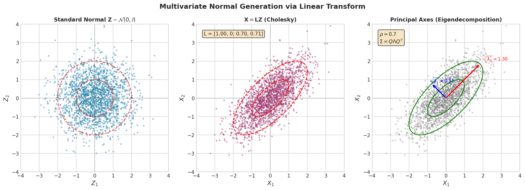
Multivariate Normal Generation. Left: 2D standard normal (\(\mathbf{Z}\)) samples form a circular cloud. Center: Cholesky transform \(\mathbf{X} = \mathbf{L}\mathbf{Z}\) stretches and rotates to match the target covariance. Right: The resulting samples follow the correct elliptical contours determined by \(\boldsymbol{\Sigma}\). Both Cholesky and eigendecomposition produce identical distributions; the choice is a matter of numerical efficiency and stability.
Practical Considerations
Boundary Handling
Several transformation methods involve \(\ln U\) where \(U \sim \text{Uniform}(0, 1)\). While \(P(U = 0) = 0\) theoretically, defensive coding prevents rare floating-point edge cases:
# Guard against U = 0
U = np.maximum(U, np.finfo(float).tiny)  # ~2.2e-308 for float64

# Alternative: use 1-U form when appropriate
# For exponential: -ln(U) or -ln(1-U) are equivalent in distribution
# but -ln(1-U) is better when U near 1 is the concern
Vectorization for Speed
All the implementations in this section use NumPy’s vectorized operations. This is crucial for performance:
import time

def timing_comparison(n=1_000_000):
    rng = np.random.default_rng(42)

    # Vectorized (fast)
    start = time.perf_counter()
    U1 = rng.random(n)
    U2 = rng.random(n)
    R = np.sqrt(-2 * np.log(np.maximum(U1, 1e-300)))
    Z = R * np.cos(2 * np.pi * U2)
    vectorized_time = time.perf_counter() - start

    # Loop (slow - don't do this!)
    start = time.perf_counter()
    Z_loop = np.empty(n)
    for i in range(min(n, 10000)):  # Only time a subset
        u1 = rng.random()
        u2 = rng.random()
        r = np.sqrt(-2 * np.log(max(u1, 1e-300)))
        Z_loop[i] = r * np.cos(2 * np.pi * u2)
    loop_time = (time.perf_counter() - start) * (n / 10000)

    print(f"Generating {n:,} normal variates:")
    print(f"  Vectorized: {1000*vectorized_time:.1f} ms")
    print(f"  Loop (est): {1000*loop_time:.0f} ms")
    print(f"  Speedup:    {loop_time/vectorized_time:.0f}×")

timing_comparison()
Generating 1,000,000 normal variates:
  Vectorized: 42.3 ms
  Loop (est): 4521 ms
  Speedup:    107×
Choosing the Right Method
Scenario |
Recommended Method |
Rationale |
|---|---|---|
Normal variates (general) |
Library function (NumPy) |
Uses optimized Ziggurat |
Normal (custom/educational) |
Polar (Marsaglia) |
Fast, no trig in inner loop |
Chi-squared (integer df) |
Sum of squared normals |
Direct, simple |
Chi-squared (non-integer df) |
Gamma generator |
Use |
Student’s t |
Normal / chi-squared ratio |
Matches definition |
Poisson (small \(\lambda < 30\)) |
Product of uniforms |
Simple, exact |
Poisson (large \(\lambda \geq 30\)) |
Normal approximation |
\(O(1)\) vs \(O(\lambda)\) |
Geometric |
Closed-form inverse CDF |
\(O(1)\), exact |
Negative Binomial (any \(r\)) |
Gamma-Poisson mixture |
Works for non-integer \(r\) |
MVN (well-conditioned) |
Cholesky |
Fastest factorization |
MVN (ill-conditioned) |
Eigendecomposition + jitter |
More robust |
Bringing It All Together
Transformation methods exploit mathematical structure to convert simple random variates (uniforms, normals) into complex distributions without iterative root-finding or general-purpose rejection sampling. The key insights are:
Geometric insight yields efficiency: The Box–Muller transform recognizes that while \(\Phi^{-1}\) has no closed form, pairs of normals have a simple polar representation. This geometric view transforms an intractable problem into an elegant solution.
Distributions form a hierarchy: Once we can generate normals efficiently, chi-squared, t, F, lognormal, and many others follow from simple arithmetic. Understanding these relationships guides algorithm design and provides verification checks.
Infinite discrete distributions have structure too: Poisson connects to exponential waiting times, Geometric has a closed-form inverse CDF, and Negative Binomial decomposes as Gamma-Poisson mixtures. These relationships transform impossible precomputation into efficient algorithms.
Multivariate normals reduce to linear algebra: The transformation \(\mathbf{X} = \boldsymbol{\mu} + \mathbf{A}\mathbf{Z}\) connects random number generation to matrix factorization. Cholesky is the workhorse; eigendecomposition handles special cases.
Numerical care pays dividends: Guarding against \(\ln(0)\), handling ill-conditioned covariance matrices, and using stable algorithms prevent rare but catastrophic failures.
Transition to Rejection Sampling
Transformation methods require that we know an explicit transformation from uniforms (or normals) to the target distribution. But what if no such transformation exists? The gamma distribution, for instance, has no simple closed-form relationship to uniforms or normals (except for integer or half-integer shape parameters).
The next section introduces rejection sampling, a universal method that can generate samples from any distribution whose density we can evaluate. The idea is elegant: propose candidates from a simpler distribution and accept or reject them probabilistically. Rejection sampling trades universality for efficiency—it always works, but may require many attempts per accepted sample. Understanding when to use transformation methods versus rejection sampling is a key skill for the computational statistician.
Key Takeaways 📝
Box–Muller transform: Converts two Uniform(0,1) variates into two independent N(0,1) variates via \(Z_1 = \sqrt{-2\ln U_1}\cos(2\pi U_2)\), \(Z_2 = \sqrt{-2\ln U_1}\sin(2\pi U_2)\). Derivation uses polar coordinates and the Jacobian.
Polar (Marsaglia) method: Eliminates trigonometric functions by rejection sampling a uniform point on the unit circle. Expected 1.27 attempts per pair; faster in compiled code.
Ziggurat algorithm: Library-standard method achieving near-constant time through layered rectangles. Conceptually elegant but complex to implement correctly—use library versions.
Distribution hierarchy: From N(0,1), derive \(\chi^2_\nu\) (sum of squares), \(t_\nu\) (ratio with chi-squared), \(F_{\nu_1,\nu_2}\) (chi-squared ratio), LogNormal (exponentiation), Rayleigh (Box–Muller radius), and Maxwell (3D magnitude).
Infinite discrete distributions: Poisson via product of uniforms (\(O(\lambda)\)) or normal approximation (\(O(1)\) for large \(\lambda\)); Geometric via closed-form inverse CDF (\(O(1)\)); Negative Binomial via Geometric sums or Gamma-Poisson mixture.
Multivariate normal: \(\mathbf{X} = \boldsymbol{\mu} + \mathbf{A}\mathbf{Z}\) where \(\mathbf{A}\mathbf{A}^T = \boldsymbol{\Sigma}\). Use Cholesky for speed, eigendecomposition for robustness or PSD matrices.
Numerical stability: Guard against \(\ln(0)\) with
np.maximum(U, tiny). Handle ill-conditioned covariances with jitter or eigenvalue clamping. Always verify PSD property before factorization.Outcome alignment: Transformation methods (Learning Outcome 1) provide efficient, exact sampling for major distributions. Understanding the normal-to-derived-distribution hierarchy and infinite discrete methods is essential for simulation-based inference throughout the course.