2.1.1. Inverse CDF Method
With a reliable supply of uniform random variates in hand—the fruit of Uniform Random Variates’s exploration of pseudo-random number generators—we now face the central question of random variable generation: how do we transform these uniform numbers into samples from other distributions?
The answer lies in one of the most elegant results in probability theory: the Probability Integral Transform. This theorem, which we previewed in our discussion of why uniform variates are “universal currency,” now receives its full mathematical treatment. It tells us that any distribution can be sampled by computing the inverse of its cumulative distribution function applied to a uniform random number. The method is universal in principle: it works for continuous, discrete, and mixed distributions alike. When the inverse CDF has a closed-form expression—as it does for exponential, Weibull, Pareto, and Cauchy distributions—implementation is immediate and efficient.
But the inverse CDF method is more than a theoretical curiosity. It is the workhorse of random number generation, the first algorithm any practitioner should consider when faced with a new distribution. Understanding when it applies, how to implement it efficiently, and when to seek alternatives is essential knowledge for computational statistics.
This section develops the inverse CDF method in full generality. We begin with the mathematical foundations—proving why the method works and what the “generalized inverse” means for distributions that lack smooth inverses. We then work through continuous distributions with closed-form inverses, deriving and implementing samplers for several important cases. For discrete distributions, we develop increasingly sophisticated algorithms: linear search, binary search, and the remarkable alias method that achieves constant-time sampling. We address numerical issues that arise in practice and identify the method’s limitations—setting the stage for rejection sampling and specialized transformations in subsequent sections.
Road Map 🧭
Understand: Why the inverse CDF method produces correctly distributed samples, with complete proofs for both continuous and discrete cases
Master: Closed-form inverse CDFs for exponential, Weibull, Pareto, Cauchy, and logistic distributions
Develop: Efficient algorithms for discrete distributions—from \(O(K)\) linear search through \(O(\log K)\) binary search to \(O(1)\) alias method
Implement: Complete Python code with attention to numerical precision and edge cases
Evaluate: When the inverse CDF method excels and when alternatives (rejection sampling, specialized transforms) are preferable
Mathematical Foundations
The inverse CDF method rests on a deep connection between the uniform distribution and all other distributions. We now develop this connection rigorously.
The Cumulative Distribution Function
For any random variable \(X\), the cumulative distribution function (CDF) \(F_X: \mathbb{R} \to [0, 1]\) is defined by:
The CDF has several fundamental properties:
Monotonicity: \(F_X\) is non-decreasing. If \(x_1 < x_2\), then \(F_X(x_1) \leq F_X(x_2)\).
Right-continuity: \(\lim_{h \to 0^+} F_X(x + h) = F_X(x)\) for all \(x\).
Limits at infinity: \(\lim_{x \to -\infty} F_X(x) = 0\) and \(\lim_{x \to \infty} F_X(x) = 1\).
For continuous random variables with density \(f_X\), the CDF is obtained by integration:
and the CDF is continuous everywhere.
For discrete random variables taking values \(x_1 < x_2 < \cdots\) with probabilities \(p_1, p_2, \ldots\), the CDF is a step function:
The CDF jumps by \(p_i\) at each value \(x_i\).
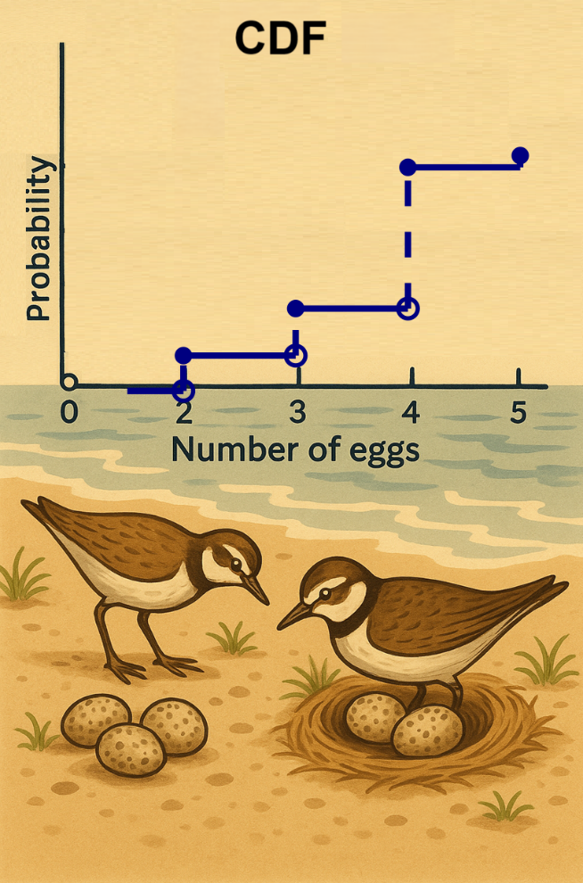
Fig. 2.1 CDF for Discrete Distributions. The cumulative distribution function of a discrete random variable is a step function with jumps at each possible value. For the killdeer clutch size example shown, the CDF maps any \(u \in (0, 1)\) to the smallest outcome \(x\) where \(F(x) \geq u\)—this is precisely the generalized inverse.
The Generalized Inverse
When \(F_X\) is continuous and strictly increasing, it has a unique inverse: \(F_X^{-1}(u)\) is the unique \(x\) such that \(F_X(x) = u\). But for discrete distributions (where \(F_X\) is a step function) or mixed distributions, the ordinary inverse does not exist. We need a more general definition.
Definition: Generalized Inverse (Quantile Function)
For any distribution function \(F: \mathbb{R} \to [0, 1]\), the generalized inverse (or quantile function) is:
This is the smallest \(x\) for which the CDF reaches or exceeds \(u\).
The generalized inverse has several important properties:
Property 1: For continuous, strictly increasing \(F\), the generalized inverse coincides with the ordinary inverse.
Property 2: For any \(F\), \(F^{-1}(u) \leq x\) if and only if \(u \leq F(x)\). This equivalence is the key to proving the inverse CDF method works.
Property 3: \(F^{-1}\) is non-decreasing and left-continuous.
Proof of Property 2:
(\(\Leftarrow\)) Suppose \(u \leq F(x)\). Then \(x \in \{t : F(t) \geq u\}\), so \(F^{-1}(u) = \inf\{t : F(t) \geq u\} \leq x\).
(\(\Rightarrow\)) Suppose \(F^{-1}(u) \leq x\). By definition, \(F^{-1}(u) = \inf\{t : F(t) \geq u\}\). By right-continuity of \(F\), \(F(F^{-1}(u)) \geq u\). Since \(F\) is non-decreasing and \(F^{-1}(u) \leq x\), we have \(F(x) \geq F(F^{-1}(u)) \geq u\). ∎
The Probability Integral Transform
With the generalized inverse defined, we can state and prove the fundamental result.
Theorem: Probability Integral Transform (Inverse Direction)
If \(U \sim \text{Uniform}(0, 1)\) and \(F\) is any distribution function, then \(X = F^{-1}(U)\) has distribution function \(F\).
Proof: We must show that \(P(X \leq x) = F(x)\) for all \(x \in \mathbb{R}\).
The final equality uses the fact that for \(U \sim \text{Uniform}(0,1)\), \(P(U \leq u) = u\) for any \(u \in [0, 1]\). ∎
This proof is remarkably general. It applies to:
Continuous distributions with smooth inverses
Discrete distributions with step-function CDFs
Mixed distributions combining point masses and continuous components
Any distribution whatsoever, provided we use the generalized inverse
The converse also holds under mild conditions:
Theorem: Probability Integral Transform (Forward Direction)
If \(X\) has a continuous CDF \(F\), then \(U = F(X) \sim \text{Uniform}(0, 1)\).
Proof: For \(u \in (0, 1)\):
where the last equality holds because \(F\) is continuous and strictly increasing on its support. ∎
Geometric Interpretation
The inverse CDF method has an intuitive geometric interpretation. Imagine the graph of the CDF \(F(x)\):
Generate a uniform random number \(u \in (0, 1)\) — a random height on the \(y\)-axis.
Draw a horizontal line at height \(u\).
Find where this line first intersects the CDF curve (or, for step functions, where it first reaches the CDF from below).
Project down to the \(x\)-axis. This is your sample \(F^{-1}(u)\).
For continuous distributions with strictly increasing CDFs, the intersection is unique. For discrete distributions, the horizontal line may intersect a “riser” of the step function; the generalized inverse picks the \(x\)-value at the top of that riser.
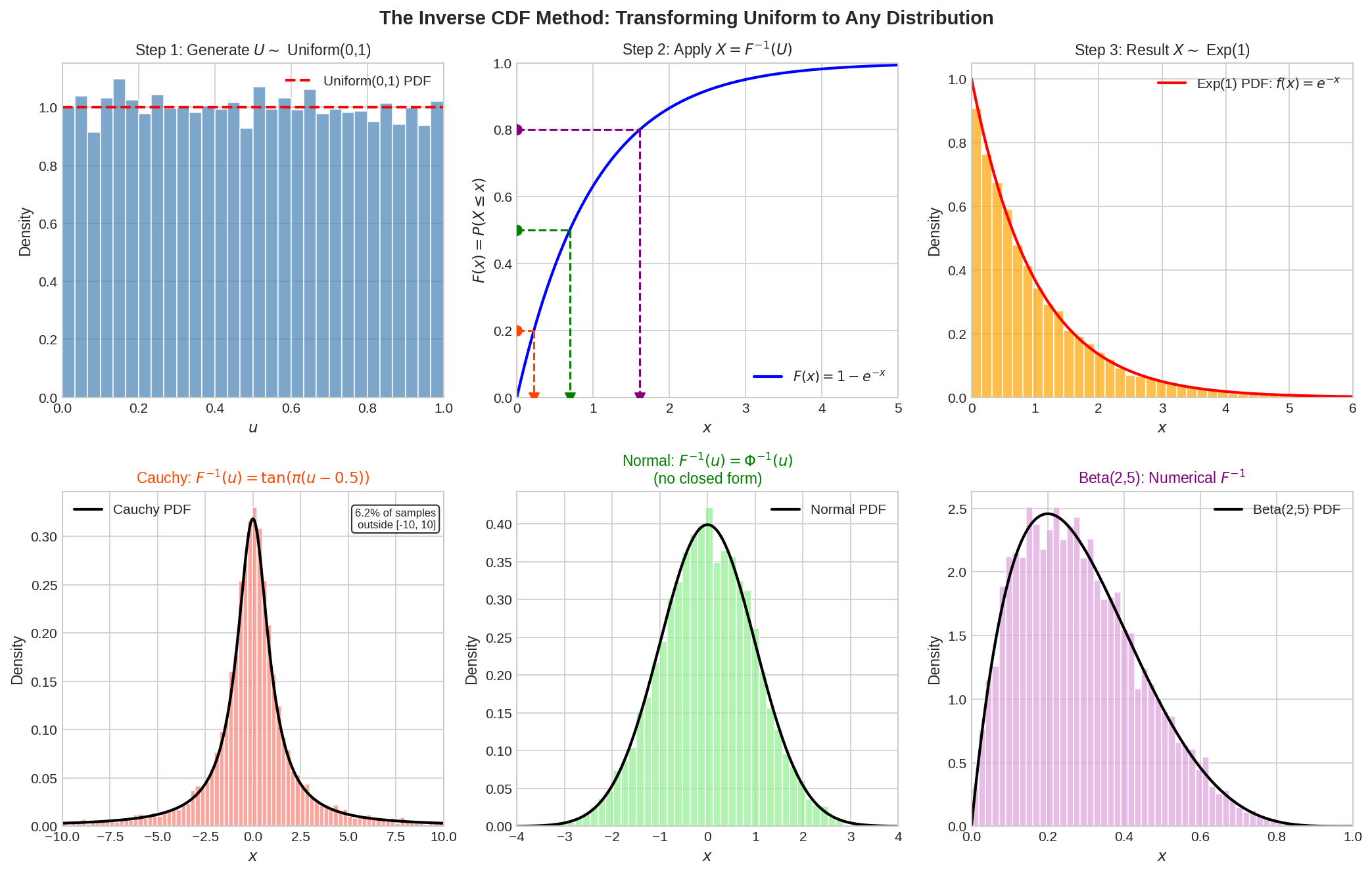
Fig. 2.2 The Inverse CDF Method: Geometric View. Top row: For an exponential distribution, we start with a uniform sample \(U\) (left), apply the inverse CDF transformation \(X = F^{-1}(U)\) (center), and obtain an exponentially distributed sample (right). The transformation “stretches” uniform samples according to where the CDF is shallow (rare values) and “compresses” where the CDF is steep (common values). Bottom row: The same process applied to three different distributions—Cauchy (heavy tails), Normal (symmetric), and Beta (flexible shape)—demonstrates the universality of the method.
Try It Yourself 🖥️ Interactive Inverse CDF Visualizations
Two interactive simulations help you build intuition for the inverse CDF method. We strongly recommend experimenting with both before proceeding.
Simulation 1: Generalized Inverse CDF Explorer
This simulation shows the geometric relationship between a CDF and its inverse side-by-side. Use it to understand why the method works:
Left panel (CDF): Shows \(F(x)\) with a horizontal line at the current \(u\) value. Watch how the vertical projection finds where \(F(x) \geq u\).
Right panel (Inverse CDF): Shows \(F^{-1}(u)\) directly as a function of \(u\). The red dot traces along this curve as you change \(u\).
Distribution selector: Switch between Continuous (Normal), Discrete (Poisson), and Mixed (Zero-inflated) to see how the generalized inverse handles each case.
Animation mode: Check “Animate u from 0 to 1” to watch how the entire range of uniform values maps to the target distribution.
Key observations to make:
For the continuous normal, both the CDF and inverse CDF are smooth curves. Moving \(u\) produces a smooth change in \(F^{-1}(u)\).
For the discrete Poisson, the CDF is a step function. Notice how the inverse CDF has flat regions (plateaus)—many different \(u\) values map to the same integer outcome. This is the generalized inverse in action: \(F^{-1}(u) = \inf\{x : F(x) \geq u\}\) finds the smallest \(x\) that “clears” the \(u\) threshold.
For the mixed zero-inflated, the CDF has a jump at zero (the point mass) followed by a continuous portion. The inverse CDF shows a flat region at \(x = 0\) for \(u \in [0, p_0]\), then becomes continuous.
Hover over either canvas to interactively set the \(u\) value—this helps you see the duality between the two representations.
Simulation 2: Inverse Transform Sampling in Action
This simulation demonstrates the sampling process itself. Watch uniform random numbers transform into samples from your chosen distribution:
Left histogram: Shows the uniform \(U \sim \text{Uniform}(0,1)\) samples accumulating. This histogram should converge to a flat (uniform) density.
Right histogram: Shows the transformed \(X = F^{-1}(U)\) samples. The gold curve overlaid is the true PDF—watch as the histogram converges to match it.
Computation display: Shows the exact arithmetic for each sample: the uniform input \(U\), the formula applied, and the output \(X\).
Distribution selector: Try Exponential, Normal, Logistic, Pareto, Cauchy, and Gamma to see different inverse CDF formulas in action.
Speed control: Slow down the animation to follow individual transformations, or speed up to see convergence faster.
Key observations to make:
The magic of transformation: Uniform samples (flat histogram on the left) become correctly distributed samples (matching the gold PDF on the right) through nothing more than arithmetic.
Concentration vs. spread: For the exponential, notice how uniform values near 0 produce small \(X\), while uniform values near 1 produce large \(X\). The inverse CDF “stretches” the uniform distribution according to where the target PDF has more or less mass.
Heavy tails: Try the Cauchy distribution and watch for occasional extreme values. These correspond to \(U\) values very close to 0 or 1, where \(\tan(\pi(U - 0.5)) \to \pm\infty\).
Sample mean convergence: Watch the “Mean” statistic. For the exponential (theoretical mean = 1), it converges nicely. For the Cauchy (no theoretical mean), it fluctuates wildly even with many samples—a vivid demonstration of heavy tails.
Formula verification: Pause the animation and verify the computation manually. For exponential with \(U = 0.3\): \(X = -\ln(1 - 0.3) = -\ln(0.7) \approx 0.357\).
Continuous Distributions with Closed-Form Inverses
The inverse CDF method is most elegant when \(F^{-1}\) has a closed-form expression. We can then generate samples with just a few arithmetic operations—typically faster than any alternative method.
The Exponential Distribution
The exponential distribution is the canonical example for the inverse CDF method. It models waiting times in Poisson processes and appears throughout reliability theory, queuing theory, and survival analysis.
Setup: \(X \sim \text{Exponential}(\lambda)\) with rate parameter \(\lambda > 0\).
CDF:
Deriving the Inverse: Solve \(F(x) = u\) for \(x\):
Simplification: Since \(U\) and \(1 - U\) have the same distribution when \(U \sim \text{Uniform}(0, 1)\), we can use either:
The second form saves one subtraction but requires care when \(u = 0\) (which occurs with probability zero but may arise from floating-point edge cases).
Example 💡 Generating Exponential Random Variables
Given: Generate 10,000 samples from \(\text{Exponential}(\lambda = 2)\).
Mathematical approach:
For \(\lambda = 2\), \(F^{-1}(u) = -\ln(1-u)/2\).
Theoretical properties:
Mean: \(\mathbb{E}[X] = 1/\lambda = 0.5\)
Variance: \(\text{Var}(X) = 1/\lambda^2 = 0.25\)
Median: \(F^{-1}(0.5) = \ln(2)/\lambda \approx 0.347\)
Python implementation:
import numpy as np

def exponential_inverse_cdf(u, rate):
    """
    Generate Exponential(rate) samples via inverse CDF.

    Uses the tail-stable form X = -log(U)/rate, avoiding (1-U).
    Since U and 1-U have the same distribution, this is equivalent
    but provides better resolution for large X values.
    """
    u = np.asarray(u, dtype=float)
    # Guard against log(0) if the RNG can return exactly 0
    u = np.maximum(u, np.finfo(float).tiny)
    return -np.log(u) / rate

# Generate samples
rng = np.random.default_rng(42)
n_samples = 10_000
rate = 2.0

U = rng.random(n_samples)
X = exponential_inverse_cdf(U, rate)

# Verify
print(f"Sample mean: {np.mean(X):.4f} (theory: {1/rate:.4f})")
print(f"Sample variance: {np.var(X, ddof=1):.4f} (theory: {1/rate**2:.4f})")
print(f"Sample median: {np.median(X):.4f} (theory: {np.log(2)/rate:.4f})")
Output:
Sample mean: 0.4976 (theory: 0.5000)
Sample variance: 0.2467 (theory: 0.2500)
Sample median: 0.3441 (theory: 0.3466)
The sample statistics closely match theoretical values, confirming the correctness of our sampler.
The Weibull Distribution
The Weibull distribution generalizes the exponential to allow for increasing or decreasing hazard rates, making it fundamental in reliability analysis.
Setup: \(X \sim \text{Weibull}(k, \lambda)\) with shape \(k > 0\) and scale \(\lambda > 0\).
CDF:
Deriving the Inverse: Solve \(F(x) = u\):
Result:
Note that when \(k = 1\), the Weibull reduces to \(\text{Exponential}(1/\lambda)\).
def weibull_inverse_cdf(u, shape, scale):
    """
    Generate Weibull(shape, scale) samples via inverse CDF.

    Uses X = scale * (-log(U))^(1/shape), the tail-stable form
    that avoids computing (1-U).
    """
    u = np.asarray(u, dtype=float)
    u = np.maximum(u, np.finfo(float).tiny)  # Guard against log(0)
    return scale * (-np.log(u)) ** (1 / shape)

# Example: Weibull(k=2, λ=1) - the Rayleigh distribution
rng = np.random.default_rng(42)
U = rng.random(10_000)
X = weibull_inverse_cdf(U, shape=2, scale=1)

print(f"Sample mean: {np.mean(X):.4f}")
print(f"Sample std: {np.std(X, ddof=1):.4f}")
The Pareto Distribution
The Pareto distribution models phenomena with “heavy tails”—situations where extreme values are more likely than a normal or exponential distribution would suggest. It appears in economics (income distribution), insurance (claim sizes), and network science (degree distributions).
Setup: \(X \sim \text{Pareto}(\alpha, x_m)\) with shape \(\alpha > 0\) and scale (minimum) \(x_m > 0\).
CDF:
Deriving the Inverse:
Result:
Since \(U\) and \(1-U\) have the same distribution, the tail-stable implementation uses:
def pareto_inverse_cdf(u, alpha, x_min):
    """
    Generate Pareto(alpha, x_min) samples via inverse CDF.

    Uses the tail-stable form X = x_min * U^(-1/alpha),
    which avoids forming (1-U) and provides better resolution
    for large X values.
    """
    u = np.asarray(u, dtype=float)
    # Guard against u=0 which would give infinity
    u = np.maximum(u, np.finfo(float).tiny)
    return x_min * u ** (-1 / alpha)

# Example: Pareto(α=2.5, x_m=1)
rng = np.random.default_rng(42)
U = rng.random(10_000)
X = pareto_inverse_cdf(U, alpha=2.5, x_min=1.0)

# For α > 1, mean = α * x_m / (α - 1)
theoretical_mean = 2.5 * 1.0 / (2.5 - 1)
print(f"Sample mean: {np.mean(X):.4f} (theory: {theoretical_mean:.4f})")
The Cauchy Distribution
The Cauchy distribution is infamous for having no mean or variance—its tails are so heavy that these moments do not exist. It arises as the ratio of two independent standard normals and appears in physics as the Lorentzian distribution.
Setup: \(X \sim \text{Cauchy}(\mu, \sigma)\) with location \(\mu\) and scale \(\sigma > 0\).
CDF:
Deriving the Inverse:
Result:
Note: At \(u = 0\) and \(u = 1\), the tangent function produces \(\pm\infty\), which is mathematically correct since the Cauchy distribution has infinite support.
def cauchy_inverse_cdf(u, loc=0, scale=1):
    """
    Generate Cauchy(loc, scale) samples via inverse CDF.

    Note: Returns ±inf at u=0 and u=1, which is mathematically correct
    since the Cauchy has infinite support.
    """
    return loc + scale * np.tan(np.pi * (u - 0.5))

# Standard Cauchy
rng = np.random.default_rng(42)
U = rng.random(10_000)
X = cauchy_inverse_cdf(U)

# The median is the location parameter
print(f"Sample median: {np.median(X):.4f} (theory: 0.0)")
# Mean doesn't exist, but sample mean will be highly variable
print(f"Sample mean: {np.mean(X):.4f} (undefined theoretically)")
The Logistic Distribution
The logistic distribution resembles the normal but has heavier tails. It appears in logistic regression and as a smooth approximation to the step function.
Setup: \(X \sim \text{Logistic}(\mu, s)\) with location \(\mu\) and scale \(s > 0\).
CDF:
Deriving the Inverse:
Result:
The function \(\text{logit}(u) = \ln(u/(1-u))\) is the inverse of the logistic (sigmoid) function.
def logistic_inverse_cdf(u, loc=0, scale=1):
    """
    Generate Logistic(loc, scale) samples via inverse CDF.

    Uses log(u) - log1p(-u) for numerical stability at both tails.
    """
    u = np.asarray(u, dtype=float)
    # Clamp to avoid exact 0 or 1
    u = np.clip(u, np.finfo(float).tiny, 1 - np.finfo(float).eps)
    # Stable logit: log(u) - log(1-u) via log1p
    return loc + scale * (np.log(u) - np.log1p(-u))

# Standard logistic
rng = np.random.default_rng(42)
U = rng.random(10_000)
X = logistic_inverse_cdf(U)

# Mean = loc, Variance = (π * scale)² / 3
print(f"Sample mean: {np.mean(X):.4f} (theory: 0.0)")
print(f"Sample variance: {np.var(X, ddof=1):.4f} (theory: {np.pi**2 / 3:.4f})")
Summary: Continuous Distributions
The following table summarizes the inverse CDF formulas for common distributions:
Distribution |
CDF \(F(x)\) |
Inverse \(F^{-1}(u)\) |
|---|---|---|
Exponential(\(\lambda\)) |
\(1 - e^{-\lambda x}\) |
\(-\ln(1-u)/\lambda\) |
Weibull(\(k, \lambda\)) |
\(1 - e^{-(x/\lambda)^k}\) |
\(\lambda(-\ln(1-u))^{1/k}\) |
Pareto(\(\alpha, x_m\)) |
\(1 - (x_m/x)^\alpha\) |
\(x_m (1-u)^{-1/\alpha}\) |
Cauchy(\(\mu, \sigma\)) |
\(\frac{1}{\pi}\arctan(\frac{x-\mu}{\sigma}) + \frac{1}{2}\) |
\(\mu + \sigma\tan(\pi(u-1/2))\) |
Logistic(\(\mu, s\)) |
\(1/(1 + e^{-(x-\mu)/s})\) |
\(\mu + s\ln(u/(1-u))\) |
Uniform(\(a, b\)) |
\((x-a)/(b-a)\) |
\(a + (b-a)u\) |
Numerical Inversion
What about distributions whose inverse CDFs have no closed form? The normal distribution is the most important example: \(\Phi^{-1}(u)\) cannot be expressed in terms of elementary functions. For such distributions, we have two options:
Numerical root-finding: Solve \(F(x) = u\) numerically for each sample.
Use specialized algorithms: Box-Muller for normals, rejection sampling, etc.
Numerical inversion is always possible but often slow. Let us examine when it is practical.
Root-Finding Approach
To compute \(F^{-1}(u)\), we solve the equation \(F(x) - u = 0\). Since \(F\) is monotonically increasing, standard root-finding methods are guaranteed to converge.
Brent’s method is particularly suitable: it combines bisection (guaranteed convergence) with faster interpolation methods (speed). SciPy provides this as scipy.optimize.brentq.
import numpy as np
from scipy import optimize, stats

def numerical_inverse_cdf(cdf_func, u, bracket=(-100, 100)):
    """
    Compute F⁻¹(u) numerically using Brent's method.

    Parameters
    ----------
    cdf_func : callable
        CDF function F(x).
    u : float or array
        Probability value(s) in (0, 1).
    bracket : tuple
        Interval [a, b] containing the root.

    Returns
    -------
    float or array
        Quantile value(s).
    """
    u = np.atleast_1d(u)
    result = np.zeros_like(u, dtype=float)

    for i, u_val in enumerate(u):
        # Solve F(x) = u, i.e., F(x) - u = 0
        result[i] = optimize.brentq(
            lambda x: cdf_func(x) - u_val,
            bracket[0], bracket[1]
        )

    return result[0] if len(result) == 1 else result

# Example: Normal distribution (for comparison with scipy.stats.norm.ppf)
normal_cdf = stats.norm.cdf

u_test = np.array([0.025, 0.5, 0.975])
numerical_quantiles = numerical_inverse_cdf(normal_cdf, u_test, bracket=(-10, 10))
exact_quantiles = stats.norm.ppf(u_test)

print("Comparison of numerical vs. exact normal quantiles:")
for u, num, exact in zip(u_test, numerical_quantiles, exact_quantiles):
    print(f"  F⁻¹({u}) = {num:.6f} (numerical) vs {exact:.6f} (exact)")
Computational cost: Brent’s method typically requires \(O(\log(1/\epsilon))\) iterations to achieve tolerance \(\epsilon\), with each iteration evaluating the CDF once. For normal samples, this is about 10-20 CDF evaluations per sample—much slower than the specialized methods we’ll see later.
When Numerical Inversion Makes Sense
Numerical inversion is practical when:
You need only a few samples: Setup costs of specialized methods may dominate.
The distribution is unusual: Custom distributions without known fast samplers.
Accuracy is paramount: Numerical inversion can achieve arbitrary precision.
Numerical inversion is impractical when:
You need many samples: The per-sample cost adds up.
A fast specialized method exists: Box-Muller for normals, ratio-of-uniforms for gammas.
The CDF is expensive to evaluate: Each sample requires multiple CDF calls.
Rule of thumb: For standard distributions, use library implementations (scipy.stats, NumPy). These use the most efficient method known for each distribution. Reserve numerical inversion for custom or unusual distributions when other methods fail.
Discrete Distributions
For discrete distributions taking values \(x_1 < x_2 < \cdots < x_K\) with probabilities \(p_1, p_2, \ldots, p_K\), the inverse CDF method still applies. The CDF is now a step function:
and the generalized inverse sets \(X = x_k\) when \(F(x_{k-1}) < U \leq F(x_k)\), where \(F(x_0) = 0\).
The challenge is computational: how do we efficiently find which “step” of the CDF our uniform value :math:`U` lands on?
We present five algorithms with different complexity trade-offs, beginning with the simplest and progressing to constant-time methods:
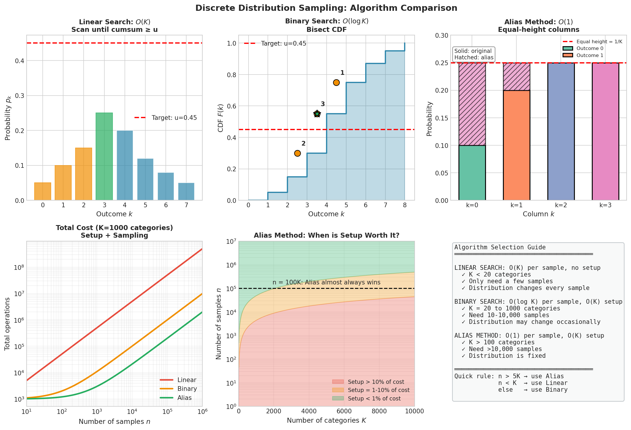
Fig. 2.3 Discrete Sampling Algorithms: Overview. Top row: Visual illustration of the three fundamental approaches. Linear search scans sequentially until cumulative probability exceeds \(U\). Binary search bisects the CDF in \(O(\log K)\) steps. The alias method constructs equal-height columns allowing \(O(1)\) lookup. Bottom row: Practical performance analysis for \(K=1000\) categories, showing when each method dominates. Additional algorithms (interpolation search, exponential doubling) are discussed below.
Linear Search: The Baseline
The simplest approach is linear search: scan through outcomes in order until the cumulative probability exceeds \(U\).
Algorithm: Linear Search
Input: Probabilities (p₁, ..., pₖ), uniform value U
Output: Sample X

1. Set cumsum = 0
2. For k = 1, 2, ..., K:
   a. cumsum = cumsum + pₖ
   b. If U ≤ cumsum, return xₖ
3. Return xₖ (fallback for numerical edge cases)
Complexity: \(O(K)\) per sample in the worst case (uniform distribution), \(O(1)\) in the best case (all mass on \(x_1\)).
def linear_search_sample(pmf, values, u):
    """
    Sample from discrete distribution via linear search.

    Parameters
    ----------
    pmf : array
        Probability mass function (must sum to 1).
    values : array
        Possible outcomes.
    u : float
        Uniform random value.

    Returns
    -------
    Sampled value.
    """
    cumsum = 0.0
    for k, p in enumerate(pmf):
        cumsum += p
        if u <= cumsum:
            return values[k]
    return values[-1]  # Fallback

# Example: biased die
pmf = np.array([0.1, 0.1, 0.1, 0.2, 0.2, 0.3])  # Heavy on 5, 6
values = np.arange(1, 7)

rng = np.random.default_rng(42)
samples = [linear_search_sample(pmf, values, rng.random()) for _ in range(10000)]
print("Sample frequencies:", np.bincount(samples, minlength=7)[1:] / 10000)
print("True probabilities:", pmf)
Binary Search: Logarithmic Time
When \(K\) is large, linear search becomes slow. We can exploit the monotonicity of the CDF to use binary search, reducing complexity to \(O(\log K)\).
The idea: precompute the cumulative probabilities \(F_k = \sum_{i=1}^k p_i\), then use binary search to find the smallest \(k\) such that \(F_k \geq U\).

Fig. 2.4 Binary Search for Discrete Sampling. For a U-shaped distribution over \(K = 16\) categories, the binary search tree (center) organizes cumulative probabilities at each node. Left panel: The CDF as a step function, with horizontal lines at key thresholds. Right panel: A complete search trace for \(U = 0.885\). Starting at the root (\(k=8, F[8]=0.500\)), we go right (since \(U > 0.500\)), then left, then right, then left, arriving at \(k=11\) in 4 steps. The algorithm pseudocode (left box) shows the standard binary search pattern.
Algorithm: Binary Search
Input: Cumulative probabilities (F₁, ..., Fₖ), uniform value U
Output: Sample index k

1. Set lo = 0, hi = K
2. While lo < hi:
   a. mid = (lo + hi) / 2
   b. If U ≤ F[mid], set hi = mid
   c. Else set lo = mid + 1
3. Return lo
Complexity: \(O(\log K)\) per sample, \(O(K)\) preprocessing to compute cumulative sums.
class DiscreteDistributionBinarySearch:
    """Discrete distribution sampler using binary search."""

    def __init__(self, pmf, values=None):
        """
        Initialize with probability mass function.

        Parameters
        ----------
        pmf : array
            Probabilities (will be normalized if needed).
        values : array, optional
            Outcome values. Defaults to 0, 1, ..., K-1.
        """
        self.pmf = np.asarray(pmf, dtype=float) / np.sum(pmf)
        self.cdf = np.cumsum(self.pmf)
        self.values = values if values is not None else np.arange(len(pmf))
        self.K = len(pmf)

    def sample(self, n_samples=1, seed=None):
        """Generate samples using binary search."""
        rng = np.random.default_rng(seed)
        U = rng.random(n_samples)

        # np.searchsorted finds insertion point - exactly what we need
        indices = np.searchsorted(self.cdf, U, side='left')

        # Clip to valid range (handles floating-point edge cases where U >= cdf[-1])
        indices = np.clip(indices, 0, self.K - 1)

        return self.values[indices]

# Example: Zipf distribution (heavy-tailed)
K = 1000
s = 2.0  # Zipf exponent
pmf = 1 / np.arange(1, K + 1) ** s
pmf /= pmf.sum()

dist = DiscreteDistributionBinarySearch(pmf)
samples = dist.sample(100_000, seed=42)

print(f"P(X = 1) = {pmf[0]:.4f}, sample frequency = {np.mean(samples == 0):.4f}")
print(f"P(X = 2) = {pmf[1]:.4f}, sample frequency = {np.mean(samples == 1):.4f}")
NumPy’s np.searchsorted implements binary search efficiently, making this approach practical for distributions with thousands or millions of outcomes.
Interpolation Search: Exploiting Structure
Binary search treats the CDF as a black box, ignoring its shape. But if we know the CDF is approximately linear (as for near-uniform distributions), we can do better. Interpolation search guesses where in the array the target value might be, based on linear interpolation.
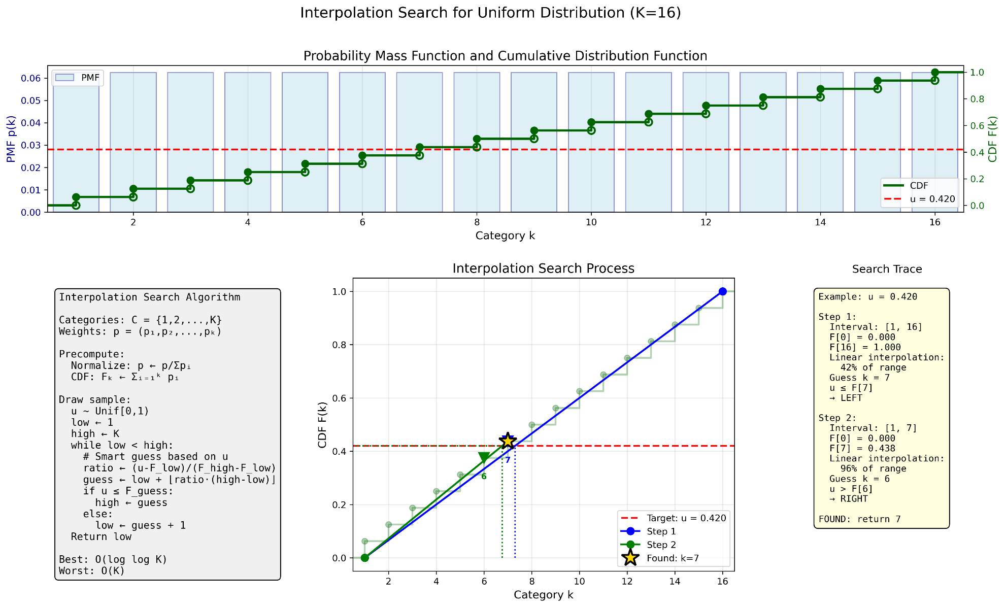
Fig. 2.5 Interpolation Search: Near-Uniform Distribution. For distributions where probability mass is spread relatively evenly, interpolation search uses linear interpolation to guess the target index. Here with \(K = 16\) categories and \(u = 0.420\), the algorithm finds the answer in just 2 steps by exploiting the near-linear CDF structure.
The Key Insight
Rather than always probing the middle of the search interval, interpolation search estimates where the target should be based on the CDF values at the interval endpoints:
This formula computes what fraction of the way through the probability range our target \(u\) lies, then maps that fraction to the index range.
Algorithm: Interpolation Search
Input: Cumulative probabilities (F₁, ..., Fₖ), uniform value U
Output: Sample index k

1. Set lo = 1, hi = K, F[0] = 0
2. While lo < hi:
   a. ratio = (U - F[lo-1]) / (F[hi] - F[lo-1])
   b. guess = lo + floor(ratio * (hi - lo))
   c. If U ≤ F[guess], set hi = guess
   d. Else set lo = guess + 1
3. Return lo
Complexity:
Best case: \(O(\log \log K)\) for uniform or near-uniform distributions
Worst case: \(O(K)\) for highly skewed distributions (where the linear assumption fails badly)
class DiscreteDistributionInterpolationSearch:
    """Discrete distribution sampler using interpolation search."""

    def __init__(self, pmf, values=None):
        """
        Initialize with probability mass function.

        Parameters
        ----------
        pmf : array
            Probabilities (will be normalized if needed).
        values : array, optional
            Outcome values. Defaults to 0, 1, ..., K-1.
        """
        self.pmf = np.asarray(pmf, dtype=float) / np.sum(pmf)
        # Prepend 0 for F[0] = 0 convention
        self.cdf = np.concatenate([[0], np.cumsum(self.pmf)])
        self.values = values if values is not None else np.arange(len(pmf))
        self.K = len(pmf)

    def _interpolation_search(self, u):
        """Find smallest k such that F[k] >= u using interpolation search."""
        lo, hi = 1, self.K

        while lo < hi:
            # Avoid division by zero
            if self.cdf[hi] <= self.cdf[lo - 1]:
                return lo

            # Linear interpolation
            ratio = (u - self.cdf[lo - 1]) / (self.cdf[hi] - self.cdf[lo - 1])
            guess = lo + int(ratio * (hi - lo))

            # Clamp guess to valid range
            guess = max(lo, min(guess, hi))

            if u <= self.cdf[guess]:
                hi = guess
            else:
                lo = guess + 1

        return lo

    def sample(self, n_samples=1, seed=None):
        """Generate samples using interpolation search."""
        rng = np.random.default_rng(seed)
        U = rng.random(n_samples)

        # Interpolation search for each U value
        indices = np.array([self._interpolation_search(u) for u in U]) - 1
        return self.values[indices]

# Example: Near-uniform distribution (interpolation search excels)
K = 1000
pmf_uniform = np.ones(K) / K

dist_interp = DiscreteDistributionInterpolationSearch(pmf_uniform)
samples = dist_interp.sample(10_000, seed=42)

print(f"Sample mean: {np.mean(samples):.1f} (theory: {(K-1)/2:.1f})")

Fig. 2.6 Interpolation Search: Skewed Distribution. For a monotonically increasing PMF (more mass on higher categories), interpolation search requires 3 steps to find \(k = 15\) for \(u = 0.780\). The linear interpolation estimates are less accurate when the CDF curves away from a straight line, but the algorithm still converges correctly.
When Interpolation Search Helps
Interpolation search shines when:
The distribution is close to uniform: \(O(\log \log K)\) expected comparisons
The CDF is approximately linear over most of its range
You need many samples from a fixed distribution (no setup cost beyond computing the CDF)
Interpolation search struggles when:
The distribution is highly skewed (Zipf, geometric): can degrade to \(O(K)\)
The probability mass is concentrated in a few categories
The CDF has sharp jumps
Practical recommendation: For general-purpose discrete sampling, binary search is safer. Use interpolation search only when you know the distribution is nearly uniform and need the extra speed.
Exponential Doubling Search
Exponential doubling (also called galloping or exponential search) combines the best of linear and binary search. It’s particularly effective when samples tend to fall in the “head” of the distribution (early categories).
The Idea: Instead of immediately binary searching the entire array, first find a rough range by doubling the search position until we overshoot, then binary search within that range.
Input: Cumulative probabilities (F₁, ..., Fₖ), uniform value U
Output: Sample index k

1. If U ≤ F[1], return 1
2. Set bound = 1
3. While bound < K and U > F[bound]:
   bound = min(2 * bound, K)
4. Binary search in range [bound/2, bound]
5. Return result
Complexity: \(O(\log k)\) where \(k\) is the result index—much better than \(O(\log K)\) when \(k \ll K\).
def exponential_doubling_search(cdf, u):
    """
    Find smallest k such that cdf[k] >= u using exponential doubling.

    Parameters
    ----------
    cdf : array
        Cumulative probabilities, cdf[0] = 0.
    u : float
        Target uniform value.

    Returns
    -------
    int
        Index k (1-indexed in the probability sense).
    """
    K = len(cdf) - 1

    if u <= cdf[1]:
        return 1

    # Exponential doubling to find upper bound
    bound = 1
    while bound < K and u > cdf[bound]:
        bound = min(2 * bound, K)

    # Binary search in [bound//2, bound]
    lo = bound // 2
    hi = bound

    while lo < hi:
        mid = (lo + hi) // 2
        if u <= cdf[mid]:
            hi = mid
        else:
            lo = mid + 1

    return lo

# Example: Head-heavy distribution (exponential doubling excels)
K = 10000
alpha = 2.0
pmf_zipf = 1 / np.arange(1, K + 1) ** alpha
pmf_zipf /= pmf_zipf.sum()
cdf_zipf = np.concatenate([[0], np.cumsum(pmf_zipf)])

# Most samples will be in early categories
rng = np.random.default_rng(42)
U = rng.random(1000)
results = [exponential_doubling_search(cdf_zipf, u) for u in U]

print(f"Median result index: {np.median(results):.0f} out of {K}")
print(f"90th percentile: {np.percentile(results, 90):.0f}")
When to Use Exponential Doubling
Head-heavy distributions (Zipf, geometric, Poisson with small λ)
When most samples fall in early categories
Adaptive scenarios where the distribution may change
The alias method still wins for truly large \(K\) with many samples, but exponential doubling provides a good middle ground with no setup cost.
The Alias Method: Constant Time
Binary search achieves \(O(\log K)\) per sample—excellent, but can we do better? The remarkable alias method, developed by Walker (1977), achieves \(O(1)\) sampling time after \(O(K)\) preprocessing.
The key insight is to restructure the probability distribution into \(K\) “columns” of equal total probability \(1/K\), where each column contains probability mass from at most two original outcomes. Sampling then requires only:
Choose a column uniformly at random: \(O(1)\)
Decide between the two outcomes in that column: \(O(1)\)
The Setup Algorithm
Imagine \(K\) cups, each of capacity \(1/K\). We pour the probability mass of each outcome into cups, filling some and leaving others partially empty. The alias method pairs each underfilled cup with an overfilled one, “topping up” the underfilled cup with probability mass from the overfilled outcome.
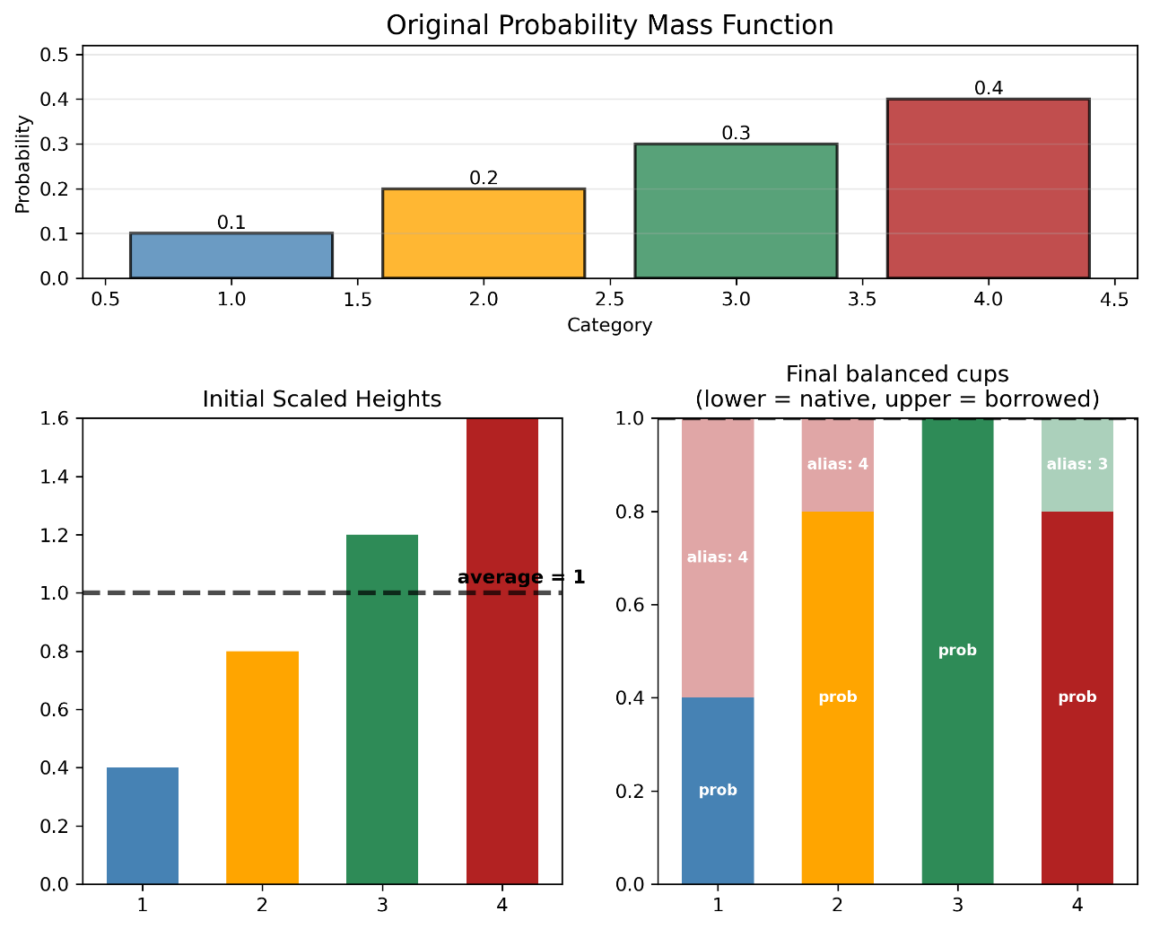
Fig. 2.7 The Alias Method: Balancing Cups. Top: Original PMF with probabilities 0.1, 0.2, 0.3, 0.4 for categories 1-4. Bottom left: After scaling by \(K=4\), the heights become 0.4, 0.8, 1.2, 1.6—some below the average of 1, others above. Bottom right: The final balanced cups, each with total height 1. Each cup contains its “native” probability (solid color) plus “borrowed” probability from an overfilled cup (lighter shading with alias label). To sample: pick a cup uniformly, then flip a coin weighted by the cup’s native vs. borrowed portions.
Input: Probabilities (p₁, ..., pₖ)
Output: Arrays prob[k] and alias[k]

1. Scale probabilities: q[k] = K * p[k]  (so Σq[k] = K)
2. Initialize:
   - small = {k : q[k] < 1}  (underfilled)
   - large = {k : q[k] ≥ 1}  (overfilled)
   - alias[k] = k for all k
3. While small and large are both non-empty:
   a. Remove j from small (underfilled)
   b. Remove ℓ from large (overfilled)
   c. Set prob[j] = q[j], alias[j] = ℓ  (record j's native prob and alias)
   d. Set q[ℓ] = q[ℓ] - (1 - q[j])  (reduce ℓ's excess)
   e. If q[ℓ] < 1, move ℓ to small; else keep in large
4. For any remaining k in small or large, set prob[k] = 1
The Sampling Algorithm
Input: Arrays prob[k] and alias[k], K
Output: Sample index

1. Generate U ~ Uniform(0, K)
2. Let i = floor(U), V = U - i  (so V ~ Uniform(0, 1))
3. If V < prob[i], return i
4. Else return alias[i]
Both steps are \(O(1)\), making sampling constant-time regardless of \(K\).
class AliasMethod:
    """
    Alias method for O(1) discrete distribution sampling.

    After O(K) setup, each sample takes O(1) time.
    """

    def __init__(self, pmf):
        """
        Initialize alias tables.

        Parameters
        ----------
        pmf : array-like
            Probability mass function (will be normalized).
        """
        pmf = np.asarray(pmf, dtype=float)
        K = len(pmf)
        pmf = pmf / pmf.sum()

        # Scale probabilities
        q = K * pmf

        # Initialize
        self.prob = np.zeros(K)
        self.alias = np.zeros(K, dtype=int)

        # Separate into small and large (with small epsilon for numerical stability)
        small = []
        large = []
        for k in range(K):
            if q[k] < 1.0 - 1e-10:
                small.append(k)
            else:
                large.append(k)

        # Build tables
        while small and large:
            j = small.pop()  # Underfilled
            ell = large.pop()  # Overfilled

            self.prob[j] = q[j]
            self.alias[j] = ell

            # Transfer mass from ℓ to j
            q[ell] = q[ell] - (1.0 - q[j])

            if q[ell] < 1.0 - 1e-10:
                small.append(ell)
            else:
                large.append(ell)

        # Remaining entries get probability 1
        while large:
            ell = large.pop()
            self.prob[ell] = 1.0
        while small:
            j = small.pop()
            self.prob[j] = 1.0

        self.K = K

    def sample(self, n_samples=1, seed=None):
        """Generate samples in O(1) per sample."""
        rng = np.random.default_rng(seed)

        # Generate uniform values in [0, K)
        U = rng.random(n_samples) * self.K

        # Extract integer and fractional parts
        i = U.astype(int)
        V = U - i  # V ~ Uniform(0, 1)

        # Handle edge case where i = K (due to floating point)
        i = np.minimum(i, self.K - 1)

        # Choose between original and alias
        return np.where(V < self.prob[i], i, self.alias[i])

# Compare performance
import time

K = 10_000
rng = np.random.default_rng(42)
pmf = rng.dirichlet(np.ones(K))  # Random distribution

# Setup
start = time.perf_counter()
alias_dist = AliasMethod(pmf)
alias_setup = time.perf_counter() - start

start = time.perf_counter()
binary_dist = DiscreteDistributionBinarySearch(pmf)
binary_setup = time.perf_counter() - start

print(f"Setup time - Alias: {alias_setup*1000:.2f} ms, Binary: {binary_setup*1000:.2f} ms")

# Sampling
n_samples = 1_000_000

start = time.perf_counter()
_ = alias_dist.sample(n_samples, seed=42)
alias_sample = time.perf_counter() - start

start = time.perf_counter()
_ = binary_dist.sample(n_samples, seed=42)
binary_sample = time.perf_counter() - start

print(f"Sample time ({n_samples:,}) - Alias: {alias_sample*1000:.2f} ms, Binary: {binary_sample*1000:.2f} ms")
Performance Comparison
With five discrete sampling algorithms now in our toolkit—linear search, binary search, interpolation search, exponential doubling, and the alias method—the natural question is: which should I use? The answer depends on distribution shape, size \(K\), and number of samples needed.
The following benchmarks compare all five methods across four distribution types, measuring both wall-clock time and iteration counts as \(K\) grows from 10 to 100,000.
Tail-Heavy Distribution (probability increases with category index):
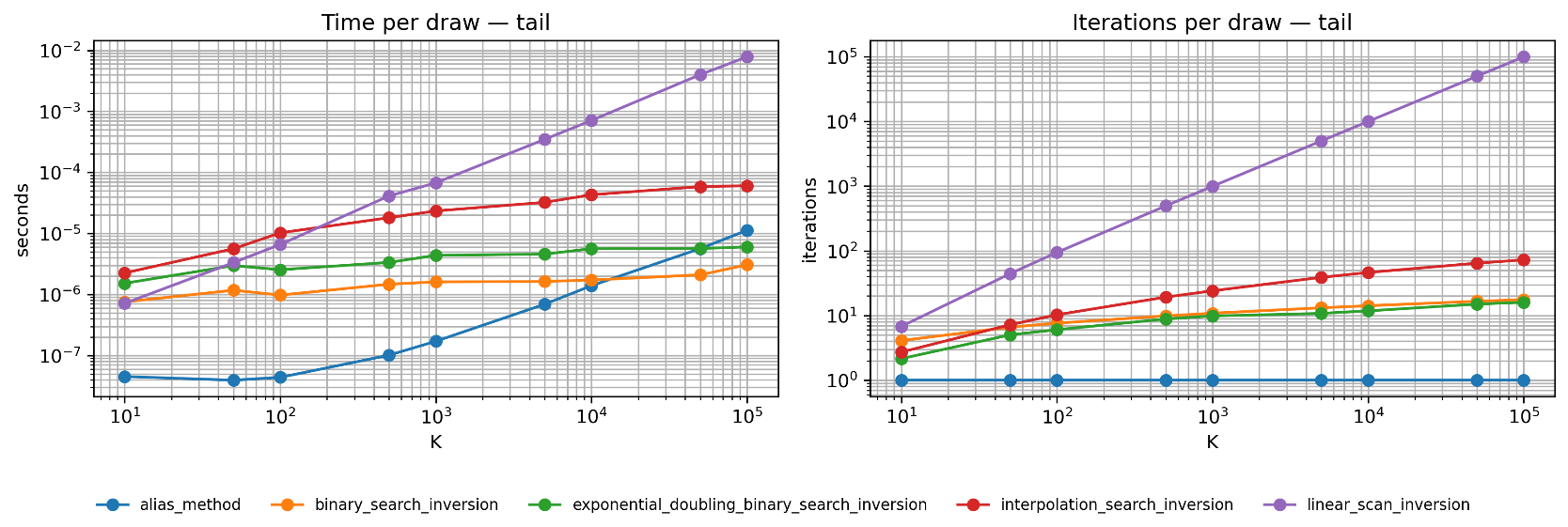
Fig. 2.8 Tail Distribution Benchmark. Left: Time per sample (seconds, log scale). Right: Iterations per sample (log scale). For tail-heavy distributions, most samples require searching toward the end of the array. Linear scan (purple) grows as \(O(K)\). Binary search (orange) and exponential doubling (green) both achieve \(O(\log K)\) but with different constants. Interpolation search (red) also grows logarithmically. The alias method (blue) maintains \(O(1)\) regardless of \(K\).
Head-Heavy Distribution (Zipf-like, probability decreases with category index):
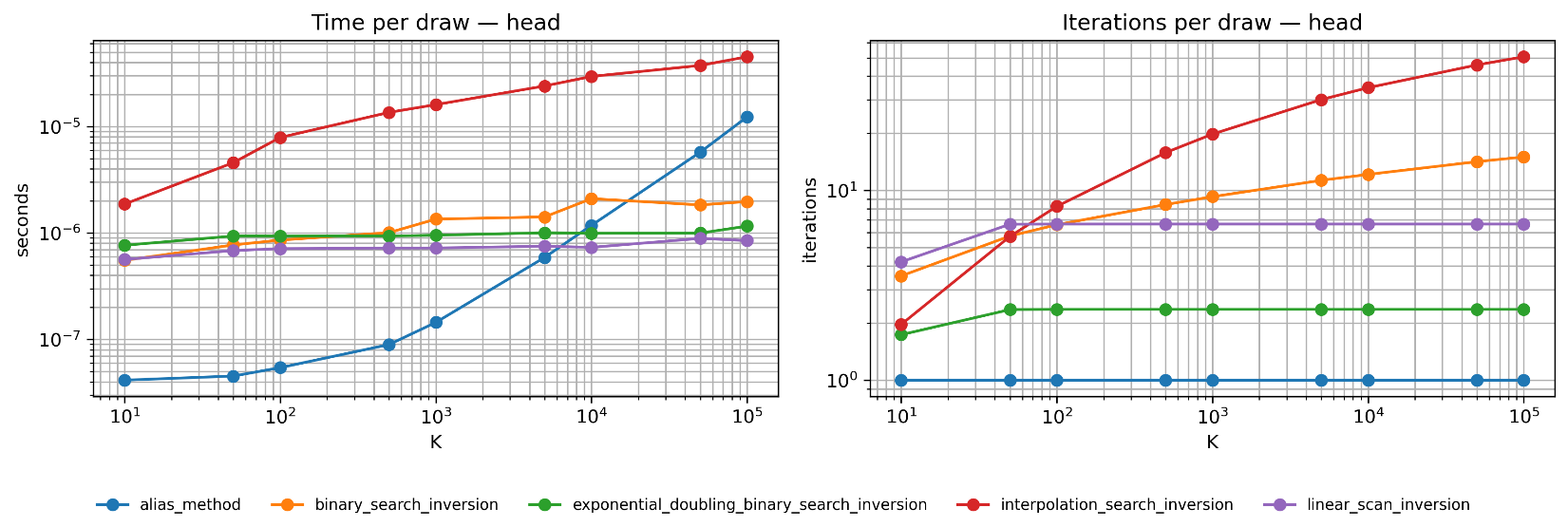
Fig. 2.9 Head-Heavy Distribution Benchmark. When probability mass concentrates in early categories, linear scan often terminates quickly (nearly constant iterations in the right panel). Exponential doubling excels here—its \(O(\log k)\) complexity (where \(k\) is the result index) means it rarely explores deep into the array. Interpolation search struggles because the CDF is highly nonlinear. The alias method remains constant.
Symmetric Distribution (U-shaped, mass at both ends):

Fig. 2.10 Symmetric Distribution Benchmark. A U-shaped distribution with mass at both head and tail represents a middle ground. Linear scan performs poorly (must traverse to the tail half the time). Binary search and exponential doubling both achieve \(O(\log K)\). The alias method’s constant time becomes increasingly advantageous as \(K\) grows.
Uniform Distribution (all categories equally likely):
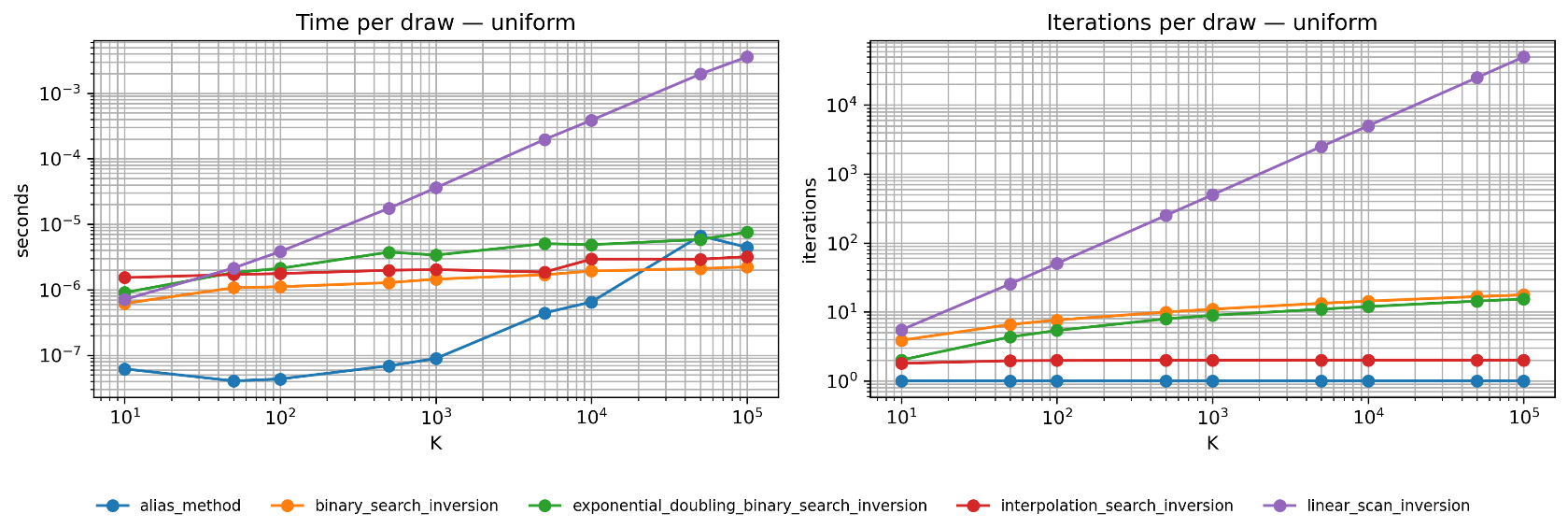
Fig. 2.11 Uniform Distribution Benchmark. This is interpolation search’s best case—the nearly linear CDF allows it to converge in \(O(\log \log K)\) iterations (notice the nearly flat red line in the right panel). For very large \(K\), interpolation search can outperform even binary search in iteration count, though per-iteration overhead may offset this advantage in wall-clock time.
Summary: Choosing the Right Algorithm
Algorithm |
Setup |
Per-Sample |
Best For |
Avoid When |
|---|---|---|---|---|
Linear scan |
\(O(1)\) |
\(O(K)\) |
\(K < 20\), extreme head-heavy |
\(K > 100\), tail-heavy |
Binary search |
\(O(K)\) |
\(O(\log K)\) |
General purpose, changing distributions |
Fixed distribution with \(n \gg K\) |
Interpolation |
\(O(K)\) |
\(O(\log\log K)\) to \(O(K)\) |
Near-uniform distributions |
Skewed distributions |
Exp. doubling |
\(O(K)\) |
\(O(\log k)\) |
Head-heavy, unknown structure |
Known uniform structure |
Alias method |
\(O(K)\) |
\(O(1)\) |
Many samples from fixed distribution |
Changing distributions, small \(n\) |
Practical recommendations:
Default choice: Binary search via
np.searchsorted—reliable \(O(\log K)\) with minimal codeHead-heavy distributions (Zipf, geometric): Exponential doubling or linear scan
Near-uniform distributions: Consider interpolation search if \(K\) is very large
Fixed distribution, many samples: Alias method pays back its setup cost when \(n > O(K)\)
Very small \(K < 20\): Linear scan’s simplicity often wins
Mixed Distributions
Real-world data often follow mixed distributions combining discrete point masses and continuous components. The inverse CDF method handles these naturally.
Zero-Inflated Distributions
A common example is the zero-inflated distribution: with probability \(p_0\), the outcome is exactly zero; otherwise, it follows a continuous distribution \(F_{\text{cont}}\).
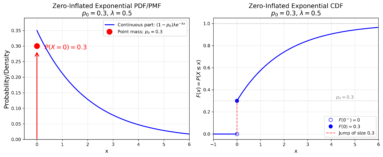
Fig. 2.12 Zero-Inflated Exponential: Structure. Left: The PDF/PMF combines a point mass at zero (red arrow, probability \(p_0 = 0.3\)) with a scaled exponential density \((1-p_0)\lambda e^{-\lambda x}\) for \(x > 0\). Right: The CDF has a jump discontinuity at zero—it jumps from \(F(0^-) = 0\) to \(F(0) = p_0\), then grows continuously following the exponential CDF scaled to the interval \([p_0, 1]\).
The CDF of a zero-inflated distribution is:
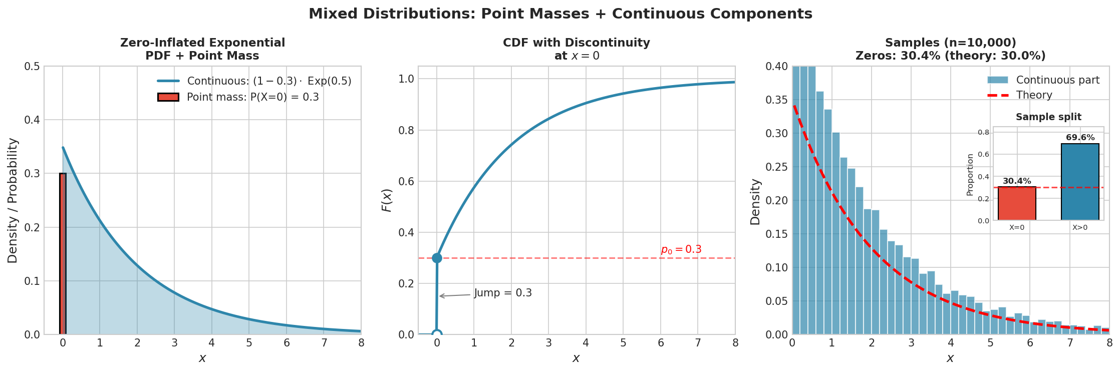
Fig. 2.13 Mixed Distributions: Sampling Verification. Left: The zero-inflated exponential has a point mass at zero (probability \(p_0 = 0.3\)) plus a continuous exponential component. Center: The CDF has a jump discontinuity of size \(p_0\) at zero, then grows continuously. Right: Sampling demonstration with the continuous part shown as a histogram matching the theoretical density. The inset bar chart confirms that the proportion of exact zeros (30.4%) closely matches the theoretical 30%.
Inverse CDF for Zero-Inflated Exponential:
For \(U \sim \text{Uniform}(0, 1)\):
If \(U \leq p_0\): return \(X = 0\)
Else: transform \(U\) to the continuous part and apply the exponential inverse
The transformation for the continuous part rescales \(U\) from \([p_0, 1]\) to \([0, 1]\):
Then \(X = F_{\text{cont}}^{-1}(U_{\text{cont}})\).
def zero_inflated_exponential(u, p_zero, rate):
    """
    Sample from zero-inflated exponential via inverse CDF.

    Parameters
    ----------
    u : float or array
        Uniform random value(s).
    p_zero : float
        Probability of structural zero.
    rate : float
        Rate of exponential component.

    Returns
    -------
    float or array
        Sample(s) from the zero-inflated distribution.
    """
    u = np.atleast_1d(u)
    result = np.zeros_like(u)

    # Points above p_zero come from the exponential
    continuous_mask = u > p_zero

    if np.any(continuous_mask):
        # Rescale U from [p_zero, 1] to [0, 1]
        u_scaled = (u[continuous_mask] - p_zero) / (1 - p_zero)
        # Guard against log(0)
        u_scaled = np.maximum(u_scaled, np.finfo(float).tiny)
        # Apply exponential inverse CDF using tail-stable form
        result[continuous_mask] = -np.log(u_scaled) / rate

    return result[0] if len(result) == 1 else result

# Verify
rng = np.random.default_rng(42)
U = rng.random(100_000)
samples = zero_inflated_exponential(U, p_zero=0.3, rate=0.5)

prop_zeros = np.mean(samples == 0)
mean_nonzero = np.mean(samples[samples > 0])

print(f"Proportion of zeros: {prop_zeros:.4f} (theory: 0.3000)")
print(f"Mean of non-zeros: {mean_nonzero:.4f} (theory: 2.0000)")
General Mixed Distributions
More generally, a mixed distribution might have \(m\) point masses at \(a_1, \ldots, a_m\) with probabilities \(\pi_1, \ldots, \pi_m\), plus a continuous component \(F_{\text{cont}}\) with weight \(\pi_{\text{cont}} = 1 - \sum_i \pi_i\).
The inverse CDF method partitions \([0, 1]\) accordingly:
def mixed_distribution_sample(u, point_masses, point_probs,
                               continuous_inverse_cdf):
    """
    Sample from a mixed discrete-continuous distribution.

    Parameters
    ----------
    u : float
        Uniform random value.
    point_masses : array
        Values with point mass.
    point_probs : array
        Probabilities of point masses.
    continuous_inverse_cdf : callable
        Inverse CDF of the continuous component.

    Returns
    -------
    float
        Sample from the mixed distribution.
    """
    cumprob = 0.0

    # Check point masses
    for mass, prob in zip(point_masses, point_probs):
        cumprob += prob
        if u <= cumprob:
            return mass

    # Continuous component
    # Rescale U to [0, 1] for the continuous part
    u_cont = (u - cumprob) / (1 - cumprob)
    return continuous_inverse_cdf(u_cont)
Practical Considerations
Numerical Precision
Several numerical issues can arise with the inverse CDF method. Understanding and mitigating them is essential for reliable implementations.
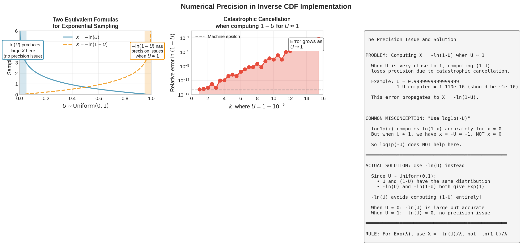
Fig. 2.14 Numerical Precision Issues. Left: Two equivalent formulas for exponential sampling—\(-\ln(U)\) and \(-\ln(1-U)\)—behave differently at the boundaries; \(-\ln(U)\) produces large samples for small \(U\) without precision issues. Center: Catastrophic cancellation when computing \(1-U\) for \(U\) near 1; each decimal digit of precision needed consumes one of float64’s ~16 available digits. Right: Explanation of why the \(-\ln(U)\) form is preferred—it places large samples where floating point has finer resolution.
1. Boundary Handling
When \(U\) is very close to 0 or 1, \(F^{-1}(U)\) may produce extreme values or overflow. For instance, \(-\ln(U) \to \infty\) as \(U \to 0\).
Mitigation: Clamp \(U\) away from exact 0. For tail-stable forms like \(-\log(U)\), use the smallest positive float to maximize tail reach:
def safe_uniform(rng, size):
    """Generate uniform values safely bounded away from 0."""
    u = rng.random(size)
    # Use smallest positive float to maximize tail reach
    return np.maximum(u, np.finfo(float).tiny)
2. Logarithms, (1-u), and What log1p Actually Fixes
Many inverse CDF formulas naturally appear in the form \(\ln(1-u)\) because they derive from the survival function. For example, for \(X \sim \text{Exponential}(\lambda)\):
In exact arithmetic this is perfectly fine. In floating-point arithmetic there are two separate concerns:
(a) Cancellation in forming \(1-U\). When \(U\) is close to 1, the quantity \(1-U\) is small, and the subtraction can lose significant digits. The function log1p(x) computes \(\ln(1+x)\) in a way that avoids the naive, accuracy-losing evaluation of log(1+x) when 1+x is close to 1. Therefore np.log1p(-u) does improve accuracy for \(\ln(1-u)\) when \(u\) is close to 1, because it avoids catastrophic cancellation in forming \(1-u\).
(b) Tail resolution near 1 (the bigger practical problem). Even if you compute \(\ln(1-U)\) accurately via log1p, sampling large exponential values requires \(U\) extremely close to 1. But IEEE-754 doubles are coarsely spaced near 1. The smallest positive gap near 1 in float64 is on the order of \(10^{-16}\), so:
This effectively truncates the far right tail and produces too few extreme values. This is a representational/granularity limitation that log1p cannot fix—it’s not a cancellation issue, it’s that the RNG cannot produce \(U\) values close enough to 1.
Best Practice for Exponential-Type Inverses
Because \(U\) and \(1-U\) have the same Uniform(0,1) distribution, rewrite the inverse in the equivalent form:
Now large \(X\) corresponds to \(U\) near 0, where floating point has much finer resolution (and can represent much smaller positive numbers). This preserves tail behavior far better in finite-precision implementations.
import numpy as np

def exponential_inverse_cdf(u, rate):
    """
    Exponential(rate) via inverse CDF, tail-stable form.

    Uses X = -log(U)/rate and avoids forming (1-U).
    """
    u = np.asarray(u, dtype=float)
    # Guard against log(0) - use smallest positive float for max tail reach
    u = np.maximum(u, np.finfo(float).tiny)
    return -np.log(u) / rate
When log1p Is the Right Tool
Use log1p when:
You genuinely need \(\ln(1-u)\) and cannot use the symmetry trick (e.g., certain non-exponential-type distributions)
You’re computing logit:
np.log(u) - np.log1p(-u)is more stable thannp.log(u / (1 - u))You’re evaluating log-survival terms where the survival function \(S(x) = 1 - F(x)\) is near 1
But log1p(-u) does not solve the tail granularity problem—it only addresses subtraction accuracy. For distributions where you can switch from log(1-u) to log(u) by symmetry (exponential, Weibull, Pareto), the symmetry-based rewrite is the most robust solution.
Common Pitfall ⚠️
Two distinct issues, two distinct fixes: (1) Cancellation when forming \(1-U\) for \(U \approx 1\)—log1p(-u) helps here. (2) Tail granularity because the RNG cannot produce \(U\) close enough to 1—log1p does not help here; the fix is to use \(-\ln(U)\) so large samples correspond to small \(U\), where floats have finer spacing.
3. CDF Evaluation Accuracy
For numerical inversion, the CDF must be evaluated accurately throughout its domain. In the tails, naive implementations may suffer from cancellation or underflow.
Example: The normal CDF \(\Phi(x)\) for \(x = 8\) is about \(1 - 6 \times 10^{-16}\)—indistinguishable from 1 in double precision. Libraries like SciPy use special functions and asymptotic expansions for accuracy in the tails.
When Not to Use Inverse CDF
The inverse CDF method is not always the best choice:
1. No Closed-Form Inverse
The normal distribution has no closed-form inverse CDF. While numerical inversion works, specialized methods like Box-Muller (Section 2.4) are faster:
produces two independent \(\mathcal{N}(0, 1)\) samples from two uniform samples—with only logarithms and trigonometric functions, no root-finding.
2. Multivariate Distributions
The inverse CDF method extends awkwardly to multiple dimensions. For a random vector \(\mathbf{X} = (X_1, \ldots, X_d)\), we would need to:
Sample \(X_1\) from its marginal
Sample \(X_2\) from its conditional given \(X_1\)
Continue sequentially…
This requires knowing all conditional distributions, which is often impractical. Rejection sampling and MCMC (Part 3) are better suited to multivariate problems.
3. Complex Dependencies
For distributions defined implicitly—such as the stationary distribution of a Markov chain or the posterior in Bayesian inference—we typically cannot even write down the CDF. Markov chain Monte Carlo methods are necessary.
Rule of Thumb: Use inverse CDF when:
The inverse has a closed-form expression, OR
You need samples from a custom discrete distribution, OR
You need only a few samples from an unusual distribution
Use other methods when:
Specialized algorithms exist (Box-Muller for normals, ratio-of-uniforms for gammas)
The distribution is multivariate
The distribution is defined implicitly
Bringing It All Together
The inverse CDF method is the theoretical foundation for random variable generation. Its power lies in universality: the same principle—transform uniform samples through the quantile function—applies to continuous, discrete, and mixed distributions alike.
For continuous distributions with tractable inverses, the method is both elegant and efficient:
Exponential, Weibull, Pareto: one logarithm, a few arithmetic operations
Cauchy, logistic: trigonometric or logarithmic functions
All achieve \(O(1)\) sampling with minimal code
For discrete distributions, we developed a hierarchy of five algorithms:
Linear search: Simple, \(O(K)\) worst case, good for small \(K\) or head-heavy distributions
Binary search: \(O(\log K)\), the general-purpose workhorse
Interpolation search: \(O(\log \log K)\) for near-uniform distributions, but degrades to \(O(K)\) for skewed ones
Exponential doubling: \(O(\log k)\) where \(k\) is the result index, excellent for head-heavy distributions
Alias method: \(O(1)\) sampling after \(O(K)\) setup, optimal for large \(K\) with many samples from a fixed distribution
For mixed distributions, the inverse CDF handles point masses and continuous components naturally by partitioning the uniform range.
Numerical precision demands attention: for exponential-type inverses, use \(-\ln(U)\) rather than \(-\ln(1-U)\) to preserve tail resolution; clamp uniforms away from boundaries; and respect the limitations of floating-point arithmetic.
Most importantly, we identified when the method fails: distributions without closed-form inverses (normals), multivariate distributions (need conditional decomposition), and implicitly defined distributions (need MCMC).
Transition to What Follows
The inverse CDF method cannot efficiently handle all distributions. Two important classes require different approaches:
Box-Muller and Related Transformations (next section): When the inverse CDF lacks a closed form but clever algebraic transformations exist, we can often find efficient alternatives. The Box-Muller transform generates normal samples from uniforms using polar coordinates—faster than numerical inversion, requiring only logarithms and trigonometric functions.
Rejection Sampling (Section 2.5): When no transformation works, we can generate samples from a simpler “proposal” distribution and accept them with probability proportional to the target density. This powerful technique requires only that we can evaluate the target density up to a normalizing constant—precisely the situation in Bayesian computation.
Together with the inverse CDF method, these techniques form a complete toolkit for random variable generation. Each has its domain of applicability; the skilled practitioner knows when to use which.
Key Takeaways 📝
Core concept: The inverse CDF method generates \(X \sim F\) by computing \(X = F^{-1}(U)\) where \(U \sim \text{Uniform}(0, 1)\). The generalized inverse \(F^{-1}(u) = \inf\{x : F(x) \geq u\}\) handles all distributions—continuous, discrete, or mixed.
Continuous distributions: When \(F^{-1}\) has closed form (exponential, Weibull, Pareto, Cauchy, logistic), sampling is \(O(1)\) with a few arithmetic operations. Derive the inverse by solving \(F(x) = u\) for \(x\).
Discrete distributions: Five algorithms with different trade-offs: linear search \(O(K)\), binary search \(O(\log K)\), interpolation search \(O(\log \log K)\) for uniform distributions, exponential doubling \(O(\log k)\) for head-heavy distributions, and the alias method \(O(1)\) after \(O(K)\) setup. Choose based on distribution shape, size \(K\), and number of samples.
Numerical precision: For exponential-type inverses, use \(-\ln(U)\) rather than \(-\ln(1-U)\) so large samples correspond to \(U \approx 0\) where floating point has finer resolution. Guard against
log(0)withnp.maximum(u, np.finfo(float).tiny).Method selection: Use inverse CDF for tractable inverses and custom discrete distributions. Use Box-Muller for normals, rejection sampling for complex densities, MCMC for implicit distributions.
Outcome alignment: This section directly addresses Learning Outcome 1 (apply simulation techniques including inverse CDF transformation) and provides the foundational random variable generation methods used throughout Monte Carlo integration, resampling, and Bayesian computation.