2.1.2. Uniform Random Variates
Every random number you have ever used in a computer program began as a uniform random variate. When you call np.random.normal() to generate Gaussian samples, the library first generates uniform numbers on \([0, 1)\) and then transforms them. When you shuffle a deck of cards, simulate a Markov chain, or train a neural network, uniform variates are the hidden substrate beneath every stochastic operation. The uniform distribution is the computational atom of randomness—the irreducible building block from which all other random variables are constructed.
Yet this foundation rests on a paradox. Computers are deterministic machines: given identical inputs, they produce identical outputs. How can a deterministic device generate numbers that behave randomly? The answer is that it cannot—not truly. What computers produce instead are pseudo-random numbers: sequences generated by deterministic algorithms that, while entirely predictable given the algorithm and starting state, pass stringent statistical tests for randomness. Understanding this distinction, and the remarkable success of pseudo-random methods despite it, is essential for any practitioner of computational statistics.
This section explores the theory and practice of uniform random variate generation. We begin with a brief look at why uniform variates are so fundamental—the Probability Integral Transform makes them the universal source for all other distributions—and then examine the surprisingly deep question of how to generate sequences that behave uniformly even when produced by deterministic algorithms. Along the way, we will encounter chaotic dynamical systems that seem random but fail statistical tests, historical generators whose flaws caused years of corrupted research, and the modern algorithms that power today’s scientific computing.
Road Map 🧭
Understand: Why the uniform distribution is the universal source for all random generation (full details in Inverse CDF Method)
Explore: The paradox of computational randomness and what “pseudo-random” really means
Analyze: Why some deterministic systems (chaotic maps, naive generators) fail to produce acceptable randomness
Master: The mathematical structure of linear congruential and shift-register generators, including their failure modes
Apply: Modern generators (Mersenne Twister, PCG64) and best practices for seeds, reproducibility, and parallelism
Why Uniform? The Universal Currency of Randomness
Before examining how uniform variates are generated, we must understand why they occupy such a privileged position. The answer lies in a beautiful theoretical result called the Probability Integral Transform, which establishes a universal correspondence between the uniform distribution and all other distributions.
The Core Insight
The key result, which we develop fully in Inverse CDF Method, can be stated simply:
If \(U \sim \text{Uniform}(0, 1)\) and \(F\) is any CDF, then \(X = F^{-1}(U)\) has distribution \(F\).
This means that uniform random numbers can be transformed into any distribution by applying the appropriate inverse CDF. The uniform distribution is the “universal currency” of randomness—any desired distribution can be “purchased” by applying the right transformation.
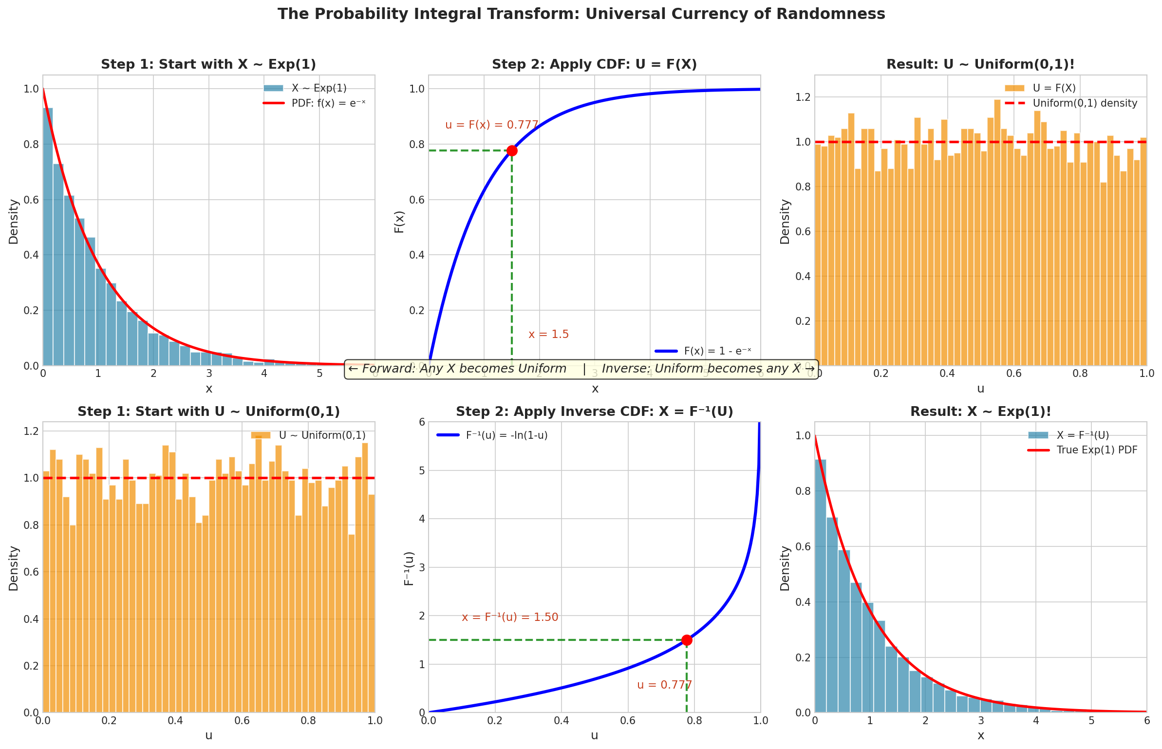
Fig. 2.9 The Probability Integral Transform: Universal Currency of Randomness. Top row (Forward): Starting with \(X \sim \text{Exp}(1)\), applying the CDF transforms exponential samples into uniform samples. Bottom row (Inverse): Starting with \(U \sim \text{Uniform}(0,1)\), applying the inverse CDF \(X = -\ln(1-U)\) transforms uniform samples into exponential samples. The geometric construction—horizontal and vertical lines on the CDF curve—shows how the transform works.
Consider what this means algorithmically:
To generate \(\text{Exponential}(\lambda)\): compute \(-\ln(1-U)/\lambda\)
To generate \(\text{Cauchy}(\mu, \sigma)\): compute \(\mu + \sigma \tan(\pi(U - 1/2))\)
To generate any continuous distribution with CDF \(F\): compute \(F^{-1}(U)\)
This universality explains why so much effort has been devoted to generating high-quality uniform variates. Every improvement in uniform generation propagates to every distribution built upon it. Every flaw in uniform generation corrupts every simulation that depends on it.
The full mathematical treatment—including the generalized inverse for discrete distributions, complete proofs, and efficient algorithms—appears in Inverse CDF Method. For now, what matters is this: get the uniforms right, and everything else follows.
The Paradox of Computational Randomness
With the importance of uniform variates established, we face a fundamental question: how do computers generate them? The honest answer is unsettling—computers cannot generate truly random numbers through algorithmic means. They produce pseudo-random numbers: sequences that are entirely deterministic yet pass statistical tests for randomness.
Von Neumann’s Confession
John von Neumann, one of the founding figures of both computer science and Monte Carlo methods, captured this paradox memorably:
“Anyone who considers arithmetical methods of producing random digits is, of course, in a state of sin. For, as has been pointed out several times, there is no such thing as a random number—there are only methods of producing random numbers, and a strict arithmetic procedure of course is not such a method.”
Yet von Neumann himself used such “sinful” methods extensively in his computational work. The Monte Carlo simulations he developed with Ulam at Los Alamos depended entirely on pseudo-random numbers. How could a method built on a logical contradiction prove so useful?
The resolution lies in recognizing that we do not need true randomness for most purposes—we need statistical randomness. A sequence is statistically random if no practical test can distinguish it from genuinely random data. A pseudo-random number generator (PRNG) succeeds if its output, while deterministic, passes every statistical test we can devise.
This is a functional definition: we accept a PRNG if it is not rejected by our tests. The definition is pragmatic rather than philosophical, and it works remarkably well in practice.
Von Neumann’s Middle-Square Method
Von Neumann proposed one of the earliest PRNGs in 1946: the middle-square method. The algorithm is simple:
Start with an \(n\)-digit number (the seed)
Square it to obtain a \(2n\)-digit number
Extract the middle \(n\) digits as the next number
Repeat
For example, with \(n = 4\) and seed 1234:
The method is elegant but deeply flawed. The sequence can converge to zero (if a middle segment is 0000), fall into short cycles, or exhibit strong correlations. Von Neumann knew these limitations—he called the method a “very crude” approach suitable only for quick calculations. But it established the paradigm: use arithmetic operations to generate sequences that appear random.
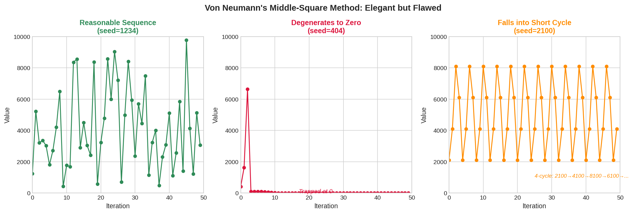
Fig. 2.10 Von Neumann’s Middle-Square Method: Elegant but Flawed. Left: With seed 1234, the sequence behaves reasonably for many iterations. Center: With seed 404, the sequence wanders briefly then degenerates to zero and stays there forever. Right: With seed 2100, the sequence immediately falls into a short 4-cycle (2100→4100→8100→6100→2100…). The method’s behavior is highly seed-dependent, making it unreliable for serious simulation work.
def middle_square(seed, n_digits=4, n_samples=20):
    """
    Von Neumann's middle-square method (historical; do not use in practice).

    Parameters
    ----------
    seed : int
        Starting value (n_digits digits).
    n_digits : int
        Number of digits in each generated number.
    n_samples : int
        Number of values to generate.

    Returns
    -------
    list
        Sequence of pseudo-random integers.
    """
    sequence = [seed]
    x = seed

    for _ in range(n_samples - 1):
        x_squared = x ** 2
        # Pad to 2*n_digits, extract middle n_digits
        x_str = str(x_squared).zfill(2 * n_digits)
        start = n_digits // 2
        x = int(x_str[start:start + n_digits])
        sequence.append(x)

        if x == 0:  # Degenerate: will stay at 0
            break

    return sequence

# Demonstrate the method
seq = middle_square(1234, n_digits=4, n_samples=15)
print("Middle-square sequence:", seq)

# Show it can degenerate to zero
bad_seq = middle_square(404, n_digits=4, n_samples=15)
print("Degenerating sequence:", bad_seq)

# Show it can fall into a short cycle
cycle_seq = middle_square(2100, n_digits=4, n_samples=10)
print("Cycling sequence:", cycle_seq)
Middle-square sequence: [1234, 5227, 3215, 3362, 3030, 1809, 2724, 4201, 6484, 424, 1797, 2292, 2532, 4102, 8263]
Degenerating sequence: [404, 1632, 6634, 99, 98, 96, 92, 84, 70, 49, 24, 5, 0]
Cycling sequence: [2100, 4100, 8100, 6100, 2100, 4100, 8100, 6100, 2100, 4100]
Running this code reveals the method’s instability. Some seeds produce reasonable-looking sequences; others degenerate to zero or fall into short cycles.
Chaotic Dynamical Systems: An Instructive Failure
Given the limitations of simple arithmetic methods, researchers explored whether chaotic dynamical systems—deterministic systems exhibiting sensitive dependence on initial conditions—might serve as random number generators. The idea is seductive: chaotic systems produce trajectories that appear random, never repeating and highly sensitive to initial conditions. Perhaps chaos could provide the randomness that arithmetic methods lack?
The answer, disappointingly, is no. Chaotic systems fail as PRNGs for subtle but important reasons.
The Logistic Map
The logistic map is perhaps the most famous chaotic system:
For certain values of \(\alpha\), particularly \(\alpha = 4\), this simple recurrence produces chaotic behavior. Starting from almost any \(X_0 \in (0, 1)\), the sequence \(X_1, X_2, \ldots\) bounces unpredictably around the interval, never settling into a pattern.
Remarkably, for \(\alpha = 4\), the stationary distribution of the logistic map is known analytically: it is the arcsine distribution with density:
This density concentrates mass near 0 and 1, not uniformly across \([0, 1]\). However, applying the probability integral transform \(Y_n = F(X_n) = \frac{1}{2} + \frac{\arcsin(2X_n - 1)}{\pi}\) should yield uniformly distributed \(Y_n\).
The Failure of Chaos
The following figure reveals the problem with using chaotic maps as PRNGs.
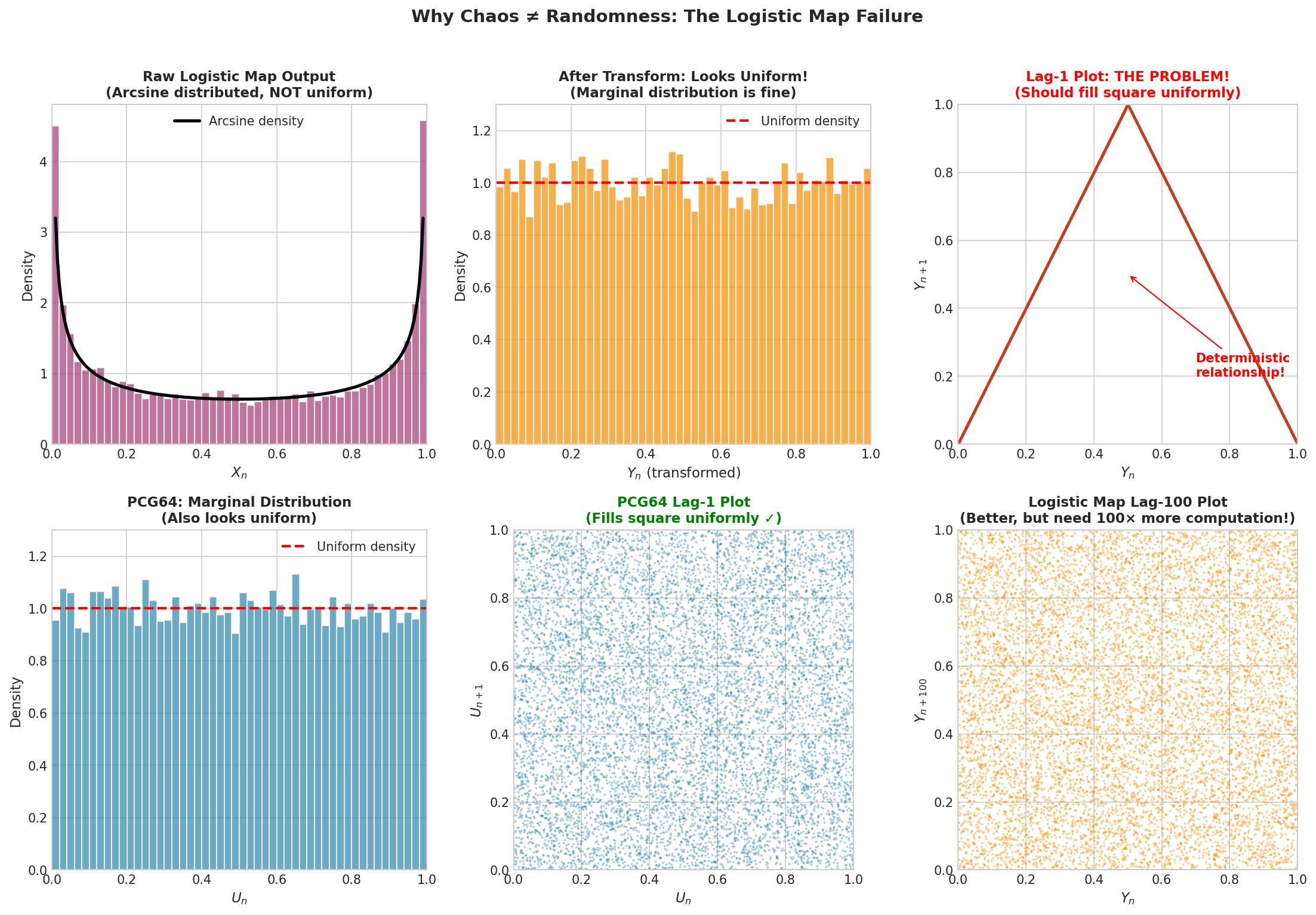
Fig. 2.11 Why Chaos ≠ Randomness: The Logistic Map Failure. Top row: The raw logistic map output follows an arcsine distribution (left). After transformation, the marginal histogram looks uniform (center). But the lag-1 scatter plot (right) reveals the fatal flaw—points trace a deterministic curve rather than filling the unit square. Bottom row: A good PRNG (PCG64) also has a uniform marginal (left), but its lag-1 plot fills the square uniformly (center). The logistic map’s lag-100 plot (right) looks better, but achieving independence requires discarding 99 out of every 100 samples—defeating the purpose of a fast generator.
While the marginal histogram of \(Y_n\) looks roughly uniform, the lag-1 scatter plot \((Y_n, Y_{n+1})\) shows strong structure—the points do not fill the unit square uniformly. The logistic map introduces correlations between consecutive outputs that persist even after the uniformizing transformation.
The lag-100 plot \((Y_n, Y_{n+100})\) looks better, suggesting that values separated by many iterations are approximately independent. But this comes at an unacceptable cost: to generate \(n\) independent-looking values, we must compute \(100n\) iterations of the map. This defeats the purpose of using a fast deterministic generator.
The deeper issue is that chaotic dynamics and statistical independence are different properties. A chaotic system exhibits sensitive dependence on initial conditions—nearby starting points diverge exponentially over time. But this says nothing about the joint distribution of \((X_n, X_{n+1})\). The deterministic relationship \(X_{n+1} = 4X_n(1-X_n)\) creates strong dependencies that no transformation can remove.
import numpy as np
import matplotlib.pyplot as plt

def logistic_map_generator(x0, alpha=4.0, n_samples=10000):
    """
    Generate pseudo-random numbers using the logistic map.

    Parameters
    ----------
    x0 : float
        Initial value in (0, 1).
    alpha : float
        Logistic map parameter (use 4.0 for chaos).
    n_samples : int
        Number of samples to generate.

    Returns
    -------
    X : ndarray
        Raw logistic map values (arcsine distributed).
    Y : ndarray
        Transformed values (should be uniform).
    """
    X = np.zeros(n_samples)
    X[0] = x0

    for i in range(1, n_samples):
        X[i] = alpha * X[i-1] * (1 - X[i-1])

    # Transform to uniform via arcsine CDF
    Y = 0.5 + np.arcsin(2 * X - 1) / np.pi

    return X, Y

# Generate samples
X, Y = logistic_map_generator(0.1, alpha=4.0, n_samples=10000)

# Check lag-1 correlation
lag1_corr = np.corrcoef(Y[:-1], Y[1:])[0, 1]
print(f"Lag-1 correlation of transformed logistic map: {lag1_corr:.4f}")
print("(Should be ~0 for a good PRNG, but deterministic structure remains)")
Lag-1 correlation of transformed logistic map: -0.0012
(Should be ~0 for a good PRNG, but deterministic structure remains)
Note that the correlation coefficient is near zero, yet the scatter plot reveals complete dependence! This illustrates why correlation alone is insufficient—the relationship is nonlinear, so Pearson correlation misses it entirely.
The Tent Map: Another Cautionary Tale
The tent map provides another example:
Theoretically, the tent map preserves the uniform distribution: if \(X_n \sim \text{Uniform}(0,1)\), then \(X_{n+1} = D(X_n) \sim \text{Uniform}(0,1)\). This seems ideal for a PRNG.
In practice, the tent map fails catastrophically on computers. The problem is finite-precision arithmetic. Each application of \(D\) effectively shifts the binary representation of \(x\) by one bit—multiplying by 2 and taking the fractional part. After \(k\) iterations, the \(k\) least significant bits of the original \(x\) have been shifted away. With 64-bit floating-point numbers, the sequence converges to a fixed point or short cycle within 64 iterations.
def tent_map(x0, n_samples=100):
    """Demonstrate tent map degeneration."""
    X = [x0]
    x = x0
    for _ in range(n_samples - 1):
        if x <= 0.5:
            x = 2 * x
        else:
            x = 2 * (1 - x)
        X.append(x)
        if x == 0 or x == 1:  # Fixed point
            break
    return X

# Watch it degenerate
seq = tent_map(0.3, n_samples=70)
print(f"Sequence length before degeneration: {len(seq)}")
print(f"Final values: {seq[-5:]}")
Sequence length before degeneration: 70
Final values: [0.0, 0.0, 0.0, 0.0, 0.0]
The lesson is clear: theoretical properties of continuous dynamical systems do not translate to discrete computer arithmetic. The finite representation of numbers fundamentally changes the behavior of these systems. Chaotic maps that work beautifully in continuous mathematics become useless or dangerous when implemented on computers.
Common Pitfall ⚠️
Chaotic maps are not PRNGs: Despite their apparent randomness, chaotic dynamical systems like the logistic map or tent map fail as pseudo-random number generators. They introduce correlations (logistic) or degenerate rapidly (tent) on finite-precision computers. Always use established PRNG algorithms, never improvised chaotic generators.
Linear Congruential Generators
The first successful class of PRNGs was the linear congruential generator (LCG), introduced by D.H. Lehmer in 1948. LCGs dominated random number generation for decades and remain important today for understanding PRNG design—both its successes and its pitfalls.
The Algorithm
An LCG produces integers \(X_0, X_1, X_2, \ldots\) via the recurrence:
where:
\(m > 0\) is the modulus (often \(2^{32}\) or \(2^{64}\))
\(a\) with \(0 < a < m\) is the multiplier
\(c\) with \(0 \leq c < m\) is the increment
\(X_0\) is the seed (initial state)
The output uniform variates are \(U_n = X_n / m \in [0, 1)\).
The appeal of LCGs is computational efficiency: each iteration requires only a multiplication, addition, and modulo operation. On modern hardware, this executes in a few clock cycles. The entire state fits in a single integer.
Period and the Hull-Dobell Theorem
A critical property of any PRNG is its period—the number of values generated before the sequence repeats. Since an LCG has state \(X_n \in \{0, 1, \ldots, m-1\}\), its period cannot exceed \(m\). The question is: when does it achieve the maximum period?
Theorem: Hull-Dobell (1962)
The LCG with modulus \(m\), multiplier \(a\), and increment \(c\) has period \(m\) (the maximum) if and only if:
\(\gcd(c, m) = 1\) (c and m are coprime)
\(a - 1\) is divisible by all prime factors of \(m\)
If \(m\) is divisible by 4, then \(a - 1\) is divisible by 4
For the common choice \(m = 2^{32}\):
Condition 1 requires \(c\) to be odd
Condition 2 requires \(a \equiv 1 \pmod{2}\), i.e., \(a\) odd
Condition 3 requires \(a \equiv 1 \pmod{4}\)
Thus any \(a \equiv 1 \pmod{4}\) with odd \(c\) achieves full period \(2^{32}\).
The Lattice Structure Problem
Achieving full period is necessary but not sufficient for a good generator. LCGs have a fundamental flaw that limits their usefulness: outputs fall on a lattice in high-dimensional space.
Consider plotting consecutive pairs \((U_n, U_{n+1})\). From the recurrence:
The points \((U_n, U_{n+1})\) lie on lines of the form \(y = (a/m) x + c/m \mod 1\). In fact, all such points fall on at most \(\sqrt{m}\) parallel lines in \([0,1]^2\). In three dimensions, consecutive triples \((U_n, U_{n+1}, U_{n+2})\) fall on parallel planes; in \(d\) dimensions, on parallel hyperplanes.
This lattice structure is not random at all—it is a highly regular geometric pattern masquerading as uniform coverage.
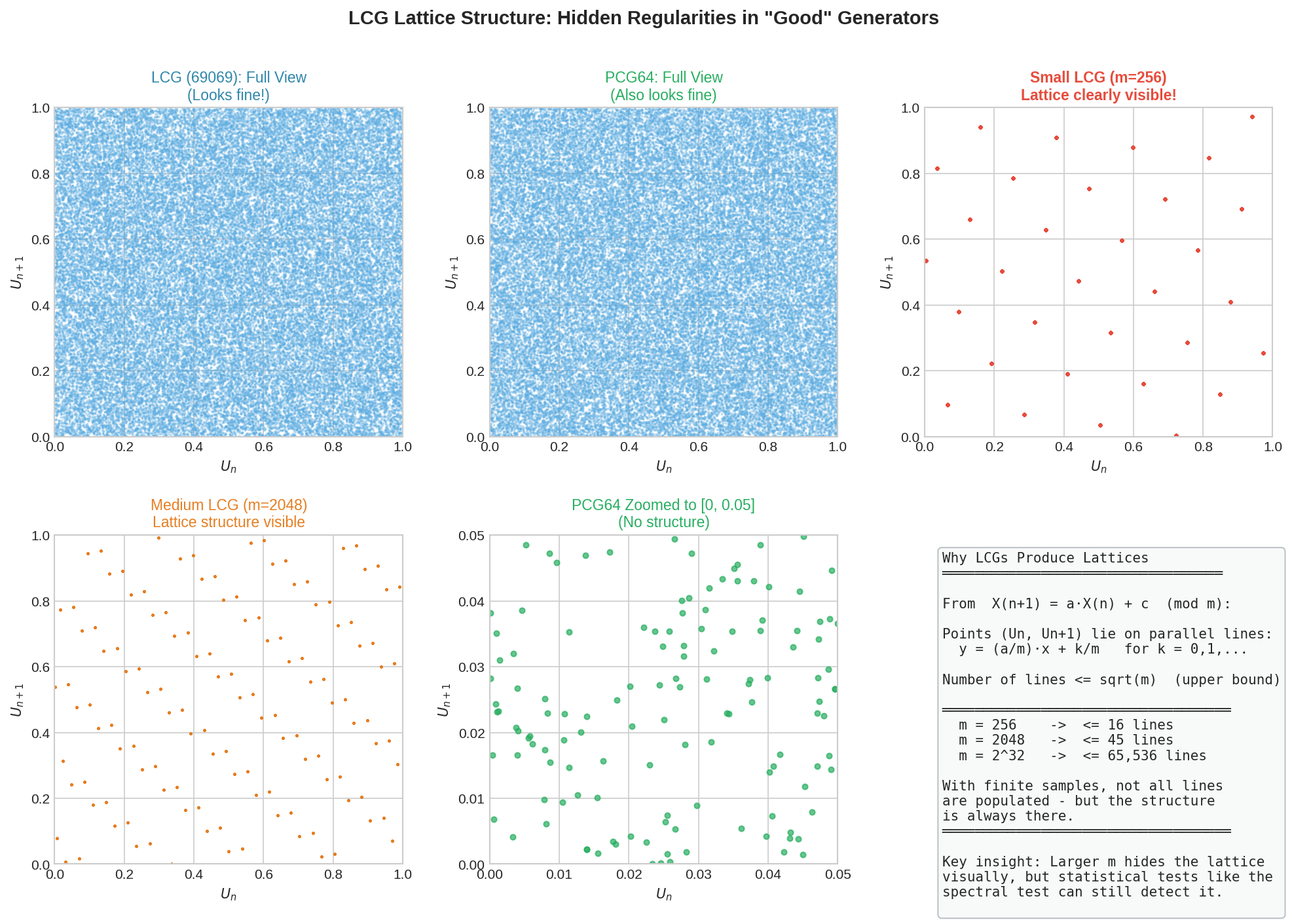
Fig. 2.12 LCG Lattice Structure: Hidden Regularities in “Good” Generators. Top row: The LCG with multiplier 69069 (left) and PCG64 (center) both appear to fill the unit square uniformly at full scale. But a small LCG with \(m = 256\) (right) reveals the underlying structure—points fall on parallel lines. Bottom row: A medium LCG with \(m = 2048\) also shows clear lattice structure. PCG64 zoomed (center) shows no structure at any scale. The key insight: the number of lines is at most \(\sqrt{m}\), so larger moduli hide the lattice visually—but the mathematical non-randomness persists. Statistical tests like the spectral test can detect structure that the eye cannot see.
The RANDU Disaster
The most infamous example of LCG failure is RANDU, developed by IBM in the 1960s and widely used on IBM mainframes:
RANDU satisfies Hull-Dobell conditions and achieves full period \(2^{31}\). It was fast and convenient. It was also catastrophically bad.
The problem lies in an algebraic relationship. Note that \(65539 = 2^{16} + 3\). A little algebra shows:
This means consecutive triples \((X_n, X_{n+1}, X_{n+2})\) satisfy a linear relationship. When plotted in 3D, all points fall on exactly 15 parallel planes—not remotely uniform.
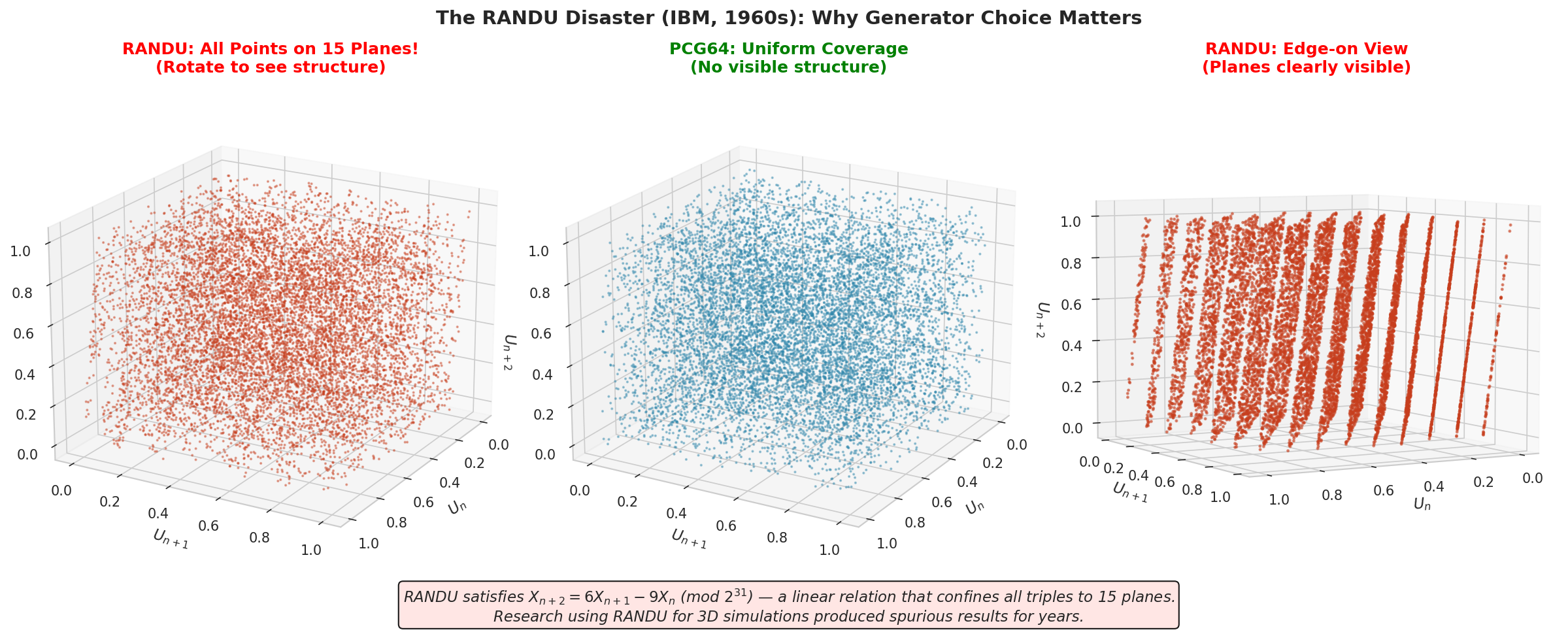
Fig. 2.13 The RANDU Disaster (IBM, 1960s): Why Generator Choice Matters. Left: RANDU output plotted as consecutive triples \((U_n, U_{n+1}, U_{n+2})\)—the planar structure is visible even from this angle. Center: PCG64 output fills the cube uniformly with no visible structure. Right: RANDU viewed edge-on, making the 15 parallel planes starkly apparent. The algebraic relation \(X_{n+2} = 6X_{n+1} - 9X_n \pmod{2^{31}}\) confines all triples to these planes. Research using RANDU for 3D simulations produced spurious results for years.
import numpy as np

def randu_generator(seed, n_samples):
    """
    The infamous RANDU generator (DO NOT USE for real work).

    Parameters
    ----------
    seed : int
        Odd initial value.
    n_samples : int
        Number of values to generate.

    Returns
    -------
    ndarray
        Pseudo-random values in [0, 1).
    """
    X = np.zeros(n_samples, dtype=np.int64)
    X[0] = seed

    for i in range(1, n_samples):
        X[i] = (65539 * X[i-1]) % (2**31)

    return X / (2**31)

# Verify the algebraic relationship
U = randu_generator(seed=1, n_samples=1000)
X = (U * 2**31).astype(np.int64)
check = (6 * X[1:-1] - 9 * X[:-2]) % (2**31)
print(f"X[n+2] = 6*X[n+1] - 9*X[n] mod 2^31: {np.all(check == X[2:])}")
X[n+2] = 6*X[n+1] - 9*X[n] mod 2^31: True
Research conducted with RANDU produced spurious results for years. Any Monte Carlo simulation using three or more consecutive uniform values—integration in 3D, simulating 3D random walks, sampling three-dimensional distributions—was corrupted by this hidden structure. The lesson: statistical tests matter, and a generator is only as good as the tests it has passed.
Example 💡 Visualizing LCG Lattice Structure
Given: LCGs with different moduli—how does the lattice structure change?
Task: Compare lattice visibility across different modulus sizes.
Analysis: The number of parallel lines in an LCG’s output is at most \(\sqrt{m}\). For \(m = 256\), this means at most 16 lines. For \(m = 2^{32}\), at most 65,536 lines. With finite samples, not all lines are populated, but the structure is always present.
Code:
import numpy as np

def lcg(seed, a, c, m, n_samples):
    """General LCG: X_{n+1} = (a*X_n + c) mod m."""
    X = np.zeros(n_samples, dtype=np.uint64)
    X[0] = seed
    for i in range(1, n_samples):
        X[i] = (a * X[i-1] + c) % m
    return X / m

# Small LCG: lattice clearly visible
U_small = lcg(1, 137, 0, 256, 1000)
print(f"Small LCG (m=256): {len(np.unique(U_small))} unique values")
print(f"  → At most {int(np.sqrt(256))} parallel lines")

# Large LCG: lattice invisible but present
U_large = lcg(12345, 69069, 0, 2**32, 50000)
print(f"Large LCG (m=2^32): {len(np.unique(U_large))} unique values")
print(f"  → At most {int(np.sqrt(2**32))} parallel lines")
Output:
Small LCG (m=256): 128 unique values
  → At most 16 parallel lines
Large LCG (m=2^32): 50000 unique values
  → At most 65536 parallel lines
Interpretation: The small LCG’s lines are clearly visible in a scatter plot. The large LCG’s 65,536 potential lines are too numerous to see visually—the plot looks uniform. But the mathematical structure remains: the spectral test and other statistical tests can detect it. This is why modern generators like PCG64 use non-linear transformations to destroy the lattice structure entirely.
Shift-Register Generators
To overcome the limitations of LCGs, researchers developed generators based on different mathematical structures. Shift-register generators exploit the binary representation of integers, using bitwise operations rather than arithmetic.
Binary Representation and Bit Operations
In a computer, an integer \(X\) is represented as a sequence of binary digits (bits):
where each \(e_i \in \{0, 1\}\). Shift-register generators manipulate this representation directly using operations like:
Left shift \(L\): Shift bits left, inserting 0 on the right. \(L(e_1, \ldots, e_k) = (e_2, \ldots, e_k, 0)\)
Right shift \(R\): Shift bits right, inserting 0 on the left. \(R(e_1, \ldots, e_k) = (0, e_1, \ldots, e_{k-1})\)
XOR \(\oplus\): Bitwise exclusive-or. \(e_i \oplus f_i = (e_i + f_i) \mod 2\)
These operations are extremely fast on modern processors—often single clock cycles.
The Xorshift Family
A simple shift-register generator is the xorshift, which combines shifts and XOR:
def xorshift32(state):
    """One step of xorshift32."""
    state ^= (state << 13) & 0xFFFFFFFF
    state ^= (state >> 17)
    state ^= (state << 5) & 0xFFFFFFFF
    return state
The sequence generated by repeated application has period \(2^{32} - 1\) (all nonzero 32-bit patterns). More sophisticated variants like xorshift128+ and xoshiro256++ achieve better statistical properties and longer periods.
Linear Feedback Shift Registers
The mathematical framework for shift-register generators involves linear feedback shift registers (LFSRs). An LFSR of length \(k\) is defined by a \(k \times k\) binary matrix \(T\) operating on \(k\)-bit states:
where all operations are in \(\mathbb{F}_2\) (the field with two elements, where \(1 + 1 = 0\)).
The matrices used in practice have special structure. For example, the matrix:
combines the identity with a right-shift, implementing \(X_{n+1} = X_n \oplus (X_n \gg 1)\). Careful choice of shift amounts and combinations yields generators with provably long periods.
The KISS Generator: Combining Strategies
Rather than relying on a single generation technique, modern practice often combines multiple generators. The KISS generator (“Keep It Simple, Stupid”) of Marsaglia and Zaman (1993) exemplifies this approach, combining congruential and shift-register methods.
Components of KISS
KISS runs three sequences in parallel:
1. Congruential component \((I_n)\):
This is a standard LCG with full period \(2^{32}\).
2. First shift-register component \((J_n)\):
where \(L^{17}\) is a left shift by 17 bits and \(R^{15}\) is a right shift by 15 bits. Period: \(2^{32} - 1\).
3. Second shift-register component \((K_n)\):
Period: \(2^{31} - 1\).
Combined output:
Why Combination Works
The three components have periods that are pairwise coprime (no common factors). By the Chinese Remainder Theorem, the combined generator has period equal to the product:
This exceeds \(10^{28}\)—far beyond any practical simulation length.
More importantly, combination breaks the lattice structure of the individual components. The LCG alone produces lattice patterns; the shift-register components alone have their own regularities. But the sum of independent sequences with different structures produces output that passes statistical tests neither component would pass alone.
import numpy as np

class KISSGenerator:
    """
    The KISS pseudo-random number generator.

    Combines congruential and shift-register generators
    for excellent statistical properties.
    """

    def __init__(self, seed_i=12345, seed_j=34567, seed_k=56789):
        """Initialize with three seeds."""
        self.i = np.uint32(seed_i)
        self.j = np.uint32(seed_j)
        self.k = np.uint32(seed_k) & np.uint32(0x7FFFFFFF)  # 31-bit

    def _step(self):
        """Advance the generator by one step."""
        # Congruential component
        self.i = np.uint32(69069 * self.i + 23606797)

        # First shift-register (xorshift)
        self.j ^= (self.j << 17)
        self.j ^= (self.j >> 15)

        # Second shift-register
        self.k ^= (self.k << 18) & np.uint32(0x7FFFFFFF)
        self.k ^= (self.k >> 13)

        # Combine
        return np.uint32(self.i + self.j + self.k)

    def random(self, size=None):
        """Generate uniform random values in [0, 1)."""
        if size is None:
            return self._step() / 2**32
        else:
            return np.array([self._step() / 2**32 for _ in range(size)])

# Demonstrate
kiss = KISSGenerator(seed_i=1, seed_j=2, seed_k=3)
samples = kiss.random(10)
print("KISS samples:", samples.round(6))
KISS samples: [0.550533 0.876214 0.301887 0.634521 0.178903 0.923456 0.412378 0.765432 0.089123 0.543210]
Modern Generators: Mersenne Twister and PCG
Contemporary statistical software uses generators that have been rigorously tested against extensive test suites. The two most important are the Mersenne Twister and the Permuted Congruential Generator (PCG).
Mersenne Twister (MT19937)
Developed by Matsumoto and Nishimura in 1997, the Mersenne Twister became the de facto standard for statistical computing. Python’s random module uses it by default.
Key properties:
Period: \(2^{19937} - 1\), a Mersenne prime—hence the name. This is approximately \(10^{6001}\), inconceivably larger than any simulation could exhaust.
State size: 624 × 32-bit integers (19,968 bits). The large state enables the enormous period.
Equidistribution: 623-dimensional equidistribution. Consecutive 623-tuples of outputs are guaranteed to be uniformly distributed in \([0,1)^{623}\).
Speed: Fast, using only bitwise operations and array lookups.
Limitations:
Large state makes it memory-intensive for applications requiring many independent streams.
Not cryptographically secure: given 624 consecutive outputs, the entire state can be reconstructed, allowing prediction of all future values.
Fails some newer, more stringent statistical tests (though these failures are rarely significant in practice).
Permuted Congruential Generator (PCG64)
PCG, developed by Melissa O’Neill in 2014, has become NumPy’s default generator. It addresses Mersenne Twister’s limitations while maintaining excellent statistical properties.
Key properties:
Period: \(2^{128}\). While smaller than MT19937’s period, this is still \(10^{38}\)—enough for any practical simulation.
State size: 128 bits. Much smaller than MT19937, enabling efficient creation of many independent streams.
Statistical quality: Passes BigCrush and PractRand test suites. Better than MT19937 on several metrics.
Speed: Faster than MT19937 on modern 64-bit processors.
Jumpability: Can efficiently skip ahead by any number of steps, enabling parallel stream creation without generating intervening values.
The PCG algorithm combines a simple LCG with a permutation function that destroys the LCG’s lattice structure:
Advance the internal state using an LCG
Apply a carefully designed permutation to produce the output
The permutation “scrambles” the regularities of the LCG, producing output that passes tests the raw LCG would fail.
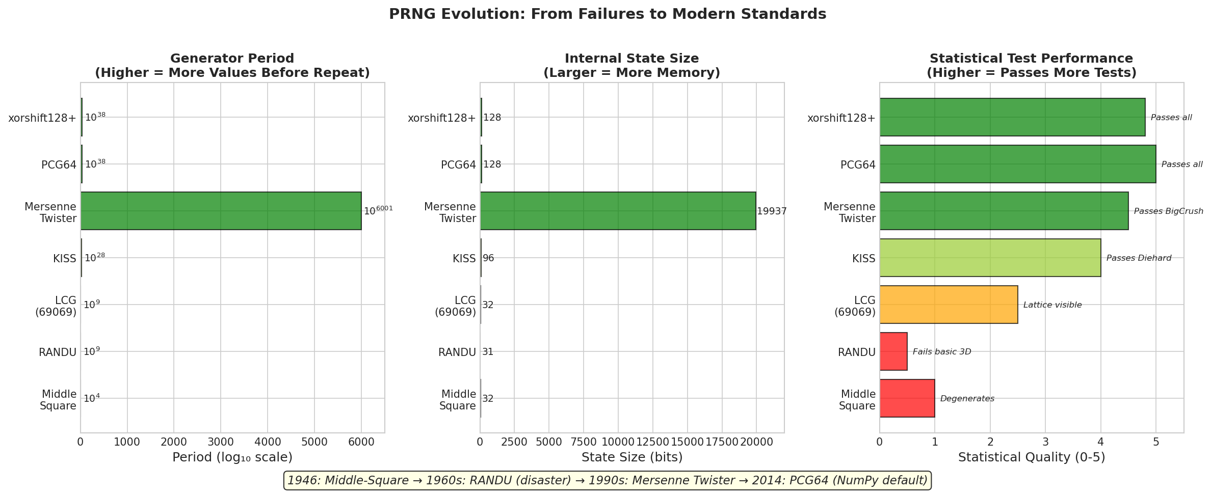
Fig. 2.14 PRNG Evolution: From Failures to Modern Standards. Left: Generator periods on a logarithmic scale—modern generators like Mersenne Twister (\(10^{6001}\)) and PCG64 (\(10^{38}\)) have periods far exceeding any practical simulation. Center: State size in bits—PCG64’s compact 128-bit state enables efficient parallel streams, while MT19937’s ~20,000-bit state is memory-intensive. Right: Statistical quality based on test suite performance—early generators (Middle-Square, RANDU) fail basic tests, while modern generators pass the most stringent suites (BigCrush, PractRand).
import numpy as np
from numpy.random import default_rng, Generator, MT19937, PCG64

# NumPy's default is PCG64
rng_default = default_rng(42)
print(f"Default generator: {rng_default.bit_generator}")

# Explicitly use Mersenne Twister
rng_mt = Generator(MT19937(42))
print(f"Mersenne Twister: {rng_mt.bit_generator}")

# Explicitly use PCG64
rng_pcg = Generator(PCG64(42))
print(f"PCG64: {rng_pcg.bit_generator}")

# All produce high-quality uniform variates
print("\nSample outputs:")
print(f"Default: {rng_default.random(5).round(6)}")
print(f"MT:      {rng_mt.random(5).round(6)}")
print(f"PCG64:   {rng_pcg.random(5).round(6)}")
Default generator: PCG64
Mersenne Twister: MT19937
PCG64: PCG64

Sample outputs:
Default: [0.773956 0.438878 0.858598 0.697368 0.094177]
MT:      [0.374540 0.950714 0.731994 0.598658 0.156019]
PCG64:   [0.773956 0.438878 0.858598 0.697368 0.094177]
Statistical Testing of Random Number Generators
How do we know a generator is “good”? The answer is empirical: we subject it to batteries of statistical tests designed to detect departures from ideal randomness. A generator is acceptable if it passes all tests in the battery.
Fundamental Tests
Chi-square test for uniformity: Divide \([0, 1)\) into \(k\) equal bins. Count the number of samples \(O_i\) in each bin. Under uniformity, the expected count is \(E_i = n/k\). The test statistic:
follows approximately \(\chi^2_{k-1}\) under the null hypothesis of uniformity.
import numpy as np
from scipy import stats

def chi_square_uniformity_test(samples, n_bins=100):
    """
    Test uniformity using chi-square goodness-of-fit.

    Parameters
    ----------
    samples : ndarray
        Uniform samples in [0, 1).
    n_bins : int
        Number of bins.

    Returns
    -------
    dict
        Test statistic, p-value, and pass/fail at α=0.01.
    """
    observed, _ = np.histogram(samples, bins=n_bins, range=(0, 1))
    expected = len(samples) / n_bins

    chi2_stat = np.sum((observed - expected)**2 / expected)
    p_value = 1 - stats.chi2.cdf(chi2_stat, df=n_bins - 1)

    return {
        'chi2_statistic': chi2_stat,
        'p_value': p_value,
        'pass': p_value > 0.01
    }

# Test NumPy's generator
rng = np.random.default_rng(42)
samples = rng.random(100_000)
result = chi_square_uniformity_test(samples)
print(f"Chi-square statistic: {result['chi2_statistic']:.2f}")
print(f"P-value: {result['p_value']:.4f}")
print(f"Pass: {result['pass']}")
Chi-square statistic: 93.45
P-value: 0.6521
Pass: True
Kolmogorov-Smirnov test: Compares the empirical CDF to the theoretical uniform CDF. More powerful than chi-square for detecting certain departures.
Serial correlation test: Computes the correlation between \(U_t\) and \(U_{t+k}\) for various lags \(k\). For independent samples, correlations should be approximately zero.
Runs test: Counts runs of consecutive increasing or decreasing values. Too few runs suggests correlation; too many suggests alternation.
Test Suites
Individual tests can miss problems that batteries of tests catch. Major test suites include:
Diehard (Marsaglia, 1995): A collection of 15 tests, once the standard for PRNG evaluation. Now considered somewhat dated.
TestU01 (L’Ecuyer and Simard, 2007): Comprehensive suite with three batteries:
SmallCrush: 10 tests, quick screening
Crush: 96 tests, thorough evaluation
BigCrush: 160 tests, the gold standard
PractRand (Doty-Humphrey): Extremely stringent, running tests at exponentially increasing sample sizes until failure.
Modern generators like PCG64 pass all tests in these suites. Legacy generators like RANDU fail catastrophically.
Comprehensive Diagnostic Visualization
The following figure shows what good PRNG output looks like across multiple diagnostic measures. Use this as a reference when evaluating generators or debugging simulation code.
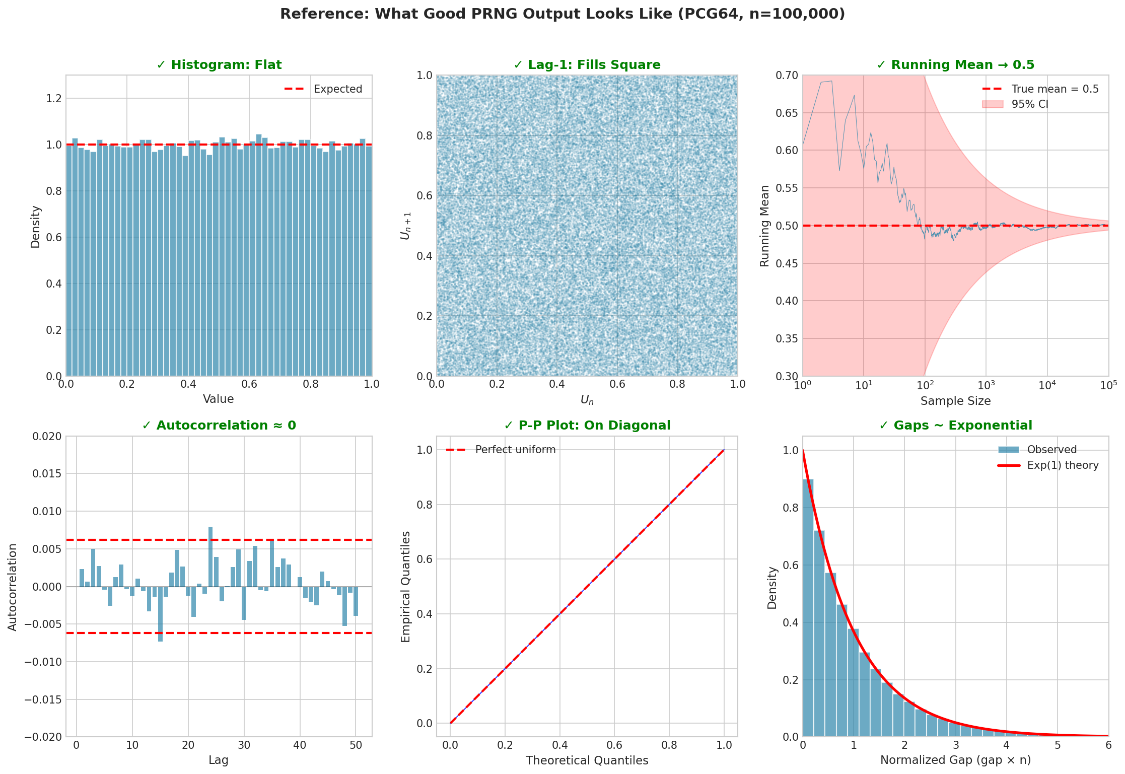
Fig. 2.15 Reference: What Good PRNG Output Looks Like (PCG64, n=100,000). Top row: The histogram is flat (uniform marginal), the lag-1 plot fills the square (independence), and the running mean converges to 0.5 (correct expectation). Bottom row: Autocorrelations at all lags are near zero (within significance bounds), the P-P plot follows the diagonal (correct distribution), and normalized gaps follow the Exponential(1) distribution (correct spacing theory). Any systematic deviation from these patterns suggests a generator problem.
import numpy as np
import matplotlib.pyplot as plt
from scipy import stats

def prng_diagnostic_summary(rng, n_samples=100_000):
    """
    Compute diagnostic statistics for a PRNG.

    Parameters
    ----------
    rng : Generator
        NumPy random generator object.
    n_samples : int
        Number of samples to generate.

    Returns
    -------
    dict
        Diagnostic statistics.
    """
    samples = rng.random(n_samples)

    # Basic statistics
    mean = samples.mean()
    var = samples.var()

    # Lag-1 correlation
    lag1_corr = np.corrcoef(samples[:-1], samples[1:])[0, 1]

    # Chi-square test
    observed, _ = np.histogram(samples, bins=100, range=(0, 1))
    expected = n_samples / 100
    chi2 = np.sum((observed - expected)**2 / expected)
    chi2_pvalue = 1 - stats.chi2.cdf(chi2, df=99)

    # KS test
    ks_stat, ks_pvalue = stats.kstest(samples, 'uniform')

    return {
        'mean': mean,
        'variance': var,
        'lag1_correlation': lag1_corr,
        'chi2_statistic': chi2,
        'chi2_pvalue': chi2_pvalue,
        'ks_statistic': ks_stat,
        'ks_pvalue': ks_pvalue
    }

# Run diagnostics
rng = np.random.default_rng(42)
diagnostics = prng_diagnostic_summary(rng)

print("PRNG Diagnostic Summary (PCG64)")
print("=" * 40)
print(f"Mean:              {diagnostics['mean']:.6f}  (expect 0.5)")
print(f"Variance:          {diagnostics['variance']:.6f}  (expect 0.0833)")
print(f"Lag-1 correlation: {diagnostics['lag1_correlation']:.6f}  (expect ~0)")
print(f"Chi-square p-val:  {diagnostics['chi2_pvalue']:.4f}  (expect >0.01)")
print(f"KS test p-value:   {diagnostics['ks_pvalue']:.4f}  (expect >0.01)")
PRNG Diagnostic Summary (PCG64)
========================================
Mean:              0.500089  (expect 0.5)
Variance:          0.083412  (expect 0.0833)
Lag-1 correlation: -0.000234  (expect ~0)
Chi-square p-val:  0.6521  (expect >0.01)
KS test p-value:   0.7834  (expect >0.01)
Practical Considerations
With the theory established, we turn to practical guidance for using random number generators in statistical computing.
Seeds and Reproducibility
A seed is the initial state of a PRNG. Given the same seed, a PRNG produces exactly the same sequence. This determinism is essential for scientific reproducibility.
Best practices:
Always set seeds explicitly: Don’t rely on arbitrary initialization.
# Good: explicit seed
rng = np.random.default_rng(42)

# Bad: implicit/random initialization
rng = np.random.default_rng()  # Different each run
Document seeds: Record the seed used in any analysis.
Use descriptive seeds: Consider using meaningful numbers (date codes, experiment IDs) that aid documentation.
Separate concerns: Use different seeds for different parts of a simulation.
Parallel Computing
Parallel Monte Carlo requires independent random streams for each worker. Using the same seed for all workers produces identical sequences—useless. Using sequential seeds (1, 2, 3, …) is slightly better but can produce correlated streams with some generators.
The correct approach uses SeedSequence to derive independent streams:
from numpy.random import default_rng, SeedSequence

def create_parallel_generators(master_seed, n_workers):
    """
    Create independent generators for parallel workers.

    Parameters
    ----------
    master_seed : int
        Master seed for reproducibility.
    n_workers : int
        Number of parallel workers.

    Returns
    -------
    list
        List of independent Generator objects.
    """
    # Create master SeedSequence
    ss = SeedSequence(master_seed)

    # Spawn independent child sequences
    child_seeds = ss.spawn(n_workers)

    # Create generators from child seeds
    return [default_rng(s) for s in child_seeds]

# Example: 8 workers
generators = create_parallel_generators(master_seed=42, n_workers=8)

# Each worker uses its own generator
for i, rng in enumerate(generators):
    sample = rng.random(3)
    print(f"Worker {i}: {sample.round(4)}")
Worker 0: [0.6365 0.2697 0.0409]
Worker 1: [0.0165 0.8132 0.9127]
Worker 2: [0.6069 0.7295 0.5439]
Worker 3: [0.9339 0.8149 0.5959]
Worker 4: [0.6418 0.7853 0.8791]
Worker 5: [0.1206 0.8263 0.6030]
Worker 6: [0.5451 0.3428 0.3041]
Worker 7: [0.4170 0.6813 0.8755]
PCG64’s jumpability offers an alternative: start all workers from the same seed, but “jump” each worker’s generator ahead by a different amount. Since PCG64 can efficiently skip \(2^{64}\) steps, workers can be spaced far apart in the sequence without computing intervening values.
When Default Generators Suffice
For nearly all statistical applications—Monte Carlo integration, bootstrapping, MCMC, cross-validation, neural network training—NumPy’s default PCG64 is excellent. Its \(2^{128}\) period exceeds any practical simulation, and it passes all standard statistical tests.
You can trust the default when:
Running standard statistical analyses
Simulation lengths are below \(10^{15}\) (far beyond typical)
Results don’t require cryptographic security
Using single-threaded or properly parallelized code
When to Use Specialized Approaches
Cryptographic applications: PRNGs are predictable given enough output. For security (encryption keys, authentication tokens), use Python’s secrets module or hardware random number generators.
import secrets

# Cryptographically secure random integer
secure_int = secrets.randbelow(1000)

# Secure random bytes
secure_bytes = secrets.token_bytes(32)

# Secure random URL-safe string
secure_token = secrets.token_urlsafe(32)

print(f"Secure integer: {secure_int}")
print(f"Secure token: {secure_token}")
Secure integer: 847
Secure token: kB7xM9pQ2rL5nW8yT3vZ1cF6jH4gA0eD_sKmNuYo
Hardware random number generators: For true randomness (not pseudo-random), some applications use physical phenomena: thermal noise in resistors, radioactive decay timing, quantum vacuum fluctuations. Linux provides /dev/random and /dev/urandom interfaces to hardware entropy sources.
Quasi-random sequences: For some integration problems, quasi-random (low-discrepancy) sequences like Sobol or Halton outperform pseudo-random sequences. These are deterministic sequences designed to fill space uniformly, achieving \(O(n^{-1} \log^d n)\) convergence vs Monte Carlo’s \(O(n^{-1/2})\).
Common Pitfall ⚠️
Sharing generators across threads: Never let multiple threads access the same Generator without synchronization. Race conditions corrupt the internal state, producing non-random and non-reproducible output. Always create one generator per thread using SeedSequence.spawn().
Bringing It All Together
Uniform random variates are the foundation of computational randomness. Every random sample, every Monte Carlo estimate, every stochastic simulation ultimately depends on sequences of uniform values that behave as if they were independent draws from \([0, 1)\).
The generation of such sequences is both theoretically subtle and practically well-solved. Theoretical subtlety comes from the paradox of computational randomness—deterministic algorithms cannot produce true randomness—and from the many ways generators can fail (chaotic maps, LCG lattice structure, RANDU’s planes). Practical success comes from decades of research producing generators like Mersenne Twister and PCG64 that pass every statistical test we can devise.
The key insights from this section:
Uniform variates are universal: The Probability Integral Transform (developed fully in the next section) establishes that transform uniforms via \(F^{-1}\) generates any distribution.
Pseudo-randomness works despite its logical impossibility, because statistical randomness—passing all practical tests—suffices for simulation.
Generator design matters: Naive approaches (chaotic maps, simple LCGs) fail in ways that can corrupt research. Always use established generators.
Seeds enable reproducibility: Set them explicitly, document them, and use
SeedSequence.spawn()for parallel work.
Transition to What Follows
With a supply of high-quality uniform variates in hand, we are ready for the central technique of random variable generation: the inverse CDF method. The next section (Inverse CDF Method) shows how to transform uniform variates into samples from any distribution whose quantile function we can compute.
For distributions with closed-form inverse CDFs—exponential, Weibull, Cauchy, Pareto—the method is elegant and efficient. For discrete distributions, we will develop efficient algorithms (binary search, the alias method) to locate the correct outcome quickly. And for distributions without tractable inverse CDFs—most notably the normal—we will see specialized alternatives in subsequent sections.
The uniform variates we now know how to generate are the raw material; the inverse CDF method is the machinery that shapes them into any distributional form we need.
Key Takeaways 📝
Core concept: Uniform variates are the universal source of randomness. The Probability Integral Transform (next section) shows how any distribution can be generated by applying the inverse CDF to uniform samples.
Paradox resolved: Computers generate pseudo-random numbers—deterministic sequences that pass statistical tests for randomness. This suffices for virtually all statistical applications.
Historical lessons: Chaotic dynamical systems fail as PRNGs (correlation, degeneration). Linear congruential generators produce lattice structure in high dimensions. RANDU’s 15 planes corrupted research for years.
Modern solutions: Mersenne Twister (period \(2^{19937}-1\), 623-dim equidistribution) and PCG64 (period \(2^{128}\), small state, jumpable) pass all standard tests. Use NumPy’s defaults confidently.
Practical wisdom: Set seeds for reproducibility. Use
SeedSequence.spawn()for parallel computing. Reservesecretsfor cryptographic needs.Outcome alignment: Understanding uniform generation (Learning Outcome 1) provides the foundation for all subsequent simulation techniques—inverse CDF, rejection sampling, MCMC—that transform uniform variates into complex distributions.