2.1.5. Rejection Sampling
The transformation methods of Transformation Methods exploit mathematical structure: Box–Muller converts uniforms to normals through polar coordinates; chi-squared emerges as a sum of squared normals; the t-distribution arises from a carefully constructed ratio. These methods are elegant and efficient—when they exist. But what happens when we need samples from a distribution with no known transformation from simple variates?
Consider the Beta distribution with general parameters \(\alpha, \beta\). No closed-form inverse CDF exists, and there is no simple transformation from uniforms or normals (except for special cases like \(\text{Beta}(1,1) = \text{Uniform}(0,1)\)). What about a posterior distribution in Bayesian inference, known only up to a normalizing constant? Or a custom density defined by a complex formula arising from domain expertise?
Rejection sampling (also called the accept-reject method) provides a universal solution. The idea, formalized by John von Neumann in 1951 in his notes “Various techniques used in connection with random digits,” is surprisingly intuitive: if we can envelope the target density with a scaled version of a simpler “proposal” density, we can generate candidates from the proposal and probabilistically accept or reject them. The accepted samples follow exactly the target distribution—no approximation, no asymptotic convergence, just exact sampling.
The conceptual roots trace back even further—to Buffon’s needle experiment (1777), one of the earliest uses of random sampling to solve a mathematical problem (estimating \(\pi\)). Von Neumann’s contribution was to generalize and formalize this intuition into a systematic method for arbitrary distributions, making it foundational to computational statistics.
The method’s power lies in its generality: rejection sampling works for any target density we can evaluate pointwise, even if the normalization constant is unknown. This makes it indispensable for Bayesian computation, where posterior densities are typically known only up to proportionality. The cost is efficiency—when the envelope fits poorly, we reject many candidates before accepting one.
This section develops rejection sampling from first principles. We begin with geometric intuition via the “dartboard” interpretation, then formalize the algorithm and prove its correctness. We analyze efficiency through acceptance rates and explore strategies for choosing good proposal distributions. Worked examples demonstrate the method for Beta distributions, truncated normals, and custom densities. We conclude by examining the method’s limitations in high dimensions, setting the stage for the Markov Chain Monte Carlo methods of later chapters.
Road Map 🧭
Understand: The geometric intuition behind rejection sampling—points uniformly distributed under a curve
Prove: Why accepted samples follow the target distribution, even with unknown normalization
Analyze: Acceptance probability as \(1/M\) and computational cost implications
Design: Strategies for choosing proposal distributions and computing the envelope constant
Implement: Efficient rejection samplers in Python with proper numerical safeguards
Recognize: When rejection sampling fails and alternatives are needed
The Dartboard Intuition
Before diving into formulas, let’s build geometric intuition for why rejection sampling works.
The Fundamental Theorem of Simulation
The theoretical foundation rests on a beautiful identity. For any probability density \(f(x)\):
This seemingly trivial observation has profound implications: the density \(f(x)\) is the marginal of a uniform distribution over the region under its curve. Formally:
Key insight: If we can sample uniformly from the region under a density curve, the \(x\)-coordinates follow that density exactly. Rejection sampling operationalizes this observation.
Points Under a Curve
Imagine plotting the probability density function \(f(x)\) of our target distribution on a coordinate plane. The area under this curve equals 1 (for a proper density). Now suppose we could somehow generate points \((x, y)\) uniformly distributed over the region under the curve—that is, uniformly over the set \(\{(x, y) : 0 \le y \le f(x)\}\).
What distribution would the \(x\)-coordinates of these points follow?
The answer is \(f(x)\) itself. To see why, consider any interval \([a, b]\). The probability that a uniformly distributed point has \(x \in [a, b]\) is proportional to the area of the region under \(f(x)\) between \(a\) and \(b\)—which is exactly \(\int_a^b f(x)\,dx\). This matches the definition of drawing from \(f\).
This observation suggests a sampling strategy: if we can generate points uniformly under \(f(x)\), we can extract their \(x\)-coordinates as samples from \(f\). But generating uniform points under an arbitrary curve is itself a non-trivial problem. Rejection sampling solves this by embedding the target region inside a larger, simpler region.
The Envelope Strategy
Suppose we have a proposal density \(g(x)\) from which we can easily sample (e.g., uniform, normal, exponential). We require that \(g(x) > 0\) wherever \(f(x) > 0\)—the proposal must “cover” the target. Furthermore, suppose we can find a constant \(M \ge 1\) such that:
The function \(M \cdot g(x)\) is called an envelope or hat function because it lies above \(f(x)\) everywhere. The region under \(f(x)\) is contained within the region under \(M \cdot g(x)\).
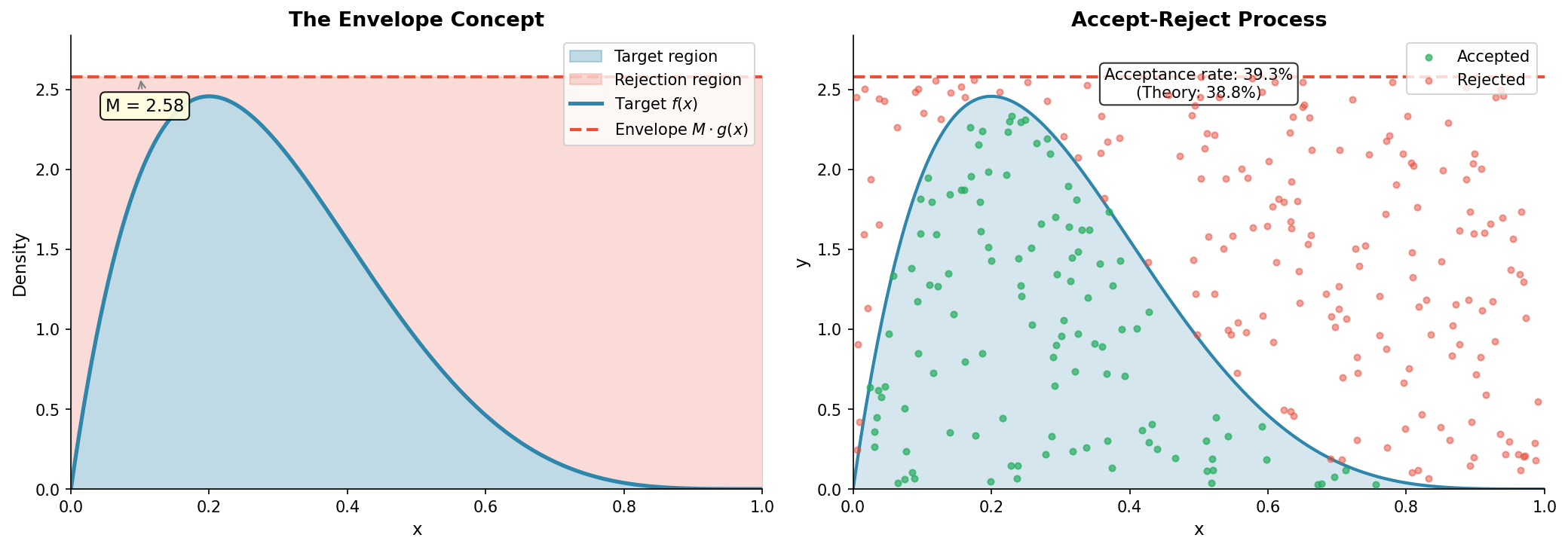
Fig. 2.36 The Envelope Concept. The target density \(f(x)\) (blue) is everywhere dominated by the envelope \(M \cdot g(x)\) (red dashed). Points uniformly distributed under the envelope will, when filtered to those under \(f(x)\), yield \(x\)-coordinates distributed according to \(f\).
Now here’s the key insight. We can easily generate points uniformly under \(M \cdot g(x)\):
Sample \(X \sim g(x)\) (a draw from the proposal distribution)
Sample \(Y \sim \text{Uniform}(0, M \cdot g(X))\) (a height uniformly distributed up to the envelope)
The pair \((X, Y)\) is uniformly distributed over the region under \(M \cdot g(x)\). If we now keep only those points with \(Y \le f(X)\)—those falling under the target density—the remaining points are uniformly distributed under \(f(x)\), and their \(x\)-coordinates follow \(f\).
The Accept-Reject Algorithm
We now formalize the geometric intuition into a precise algorithm.
Algorithm Statement
- Given:
Target density \(f(x)\), possibly known only up to a normalizing constant
Proposal density \(g(x)\) from which we can sample directly
Envelope constant \(M\) such that \(f(x) \le M \cdot g(x)\) for all \(x\)
Algorithm (Accept-Reject Method)
To generate one sample from f(x):

1. REPEAT:
   a. Draw X ~ g(x)                              [sample from proposal]
   b. Draw U ~ Uniform(0, 1)                     [independent uniform]
   c. Compute acceptance probability:
      α(X) = f(X) / [M · g(X)]
   d. IF U ≤ α(X):
      ACCEPT X and RETURN X
      ELSE:
      REJECT X and continue to next iteration

2. The returned X is an exact draw from f(x)
The key observation is that we don’t actually need to generate \(Y = U \cdot M \cdot g(X)\) explicitly. The condition \(Y \le f(X)\) is equivalent to \(U \cdot M \cdot g(X) \le f(X)\), which simplifies to \(U \le f(X) / [M \cdot g(X)] = \alpha(X)\).
Proof of Correctness
We now prove that accepted samples follow the target distribution \(f(x)\).
Theorem (Correctness of Accept-Reject). If \(f(x) \le M \cdot g(x)\) for all \(x\), then the accepted value \(X\) from the accept-reject algorithm has density \(f(x) / \int f(t)\,dt\).
Proof. Consider a single iteration. We generate \(X \sim g(x)\) and \(U \sim \text{Uniform}(0,1)\), accepting if \(U \le f(X)/[M \cdot g(X)]\).
For any measurable set \(A\):
The overall probability of acceptance is:
where \(C = \int f(x)\,dx\) is the normalizing constant of \(f\) (which equals 1 if \(f\) is already normalized).
By Bayes’ theorem:
This is exactly the probability that a random variable with density \(f(x)/C\) lies in \(A\). ∎
Key insight: The normalization constant \(C\) cancels in the acceptance ratio. We never need to compute \(\int f(x)\,dx\)—rejection sampling works even when \(f\) is known only up to proportionality.
Efficiency Analysis
Not every proposed sample is accepted. Understanding the acceptance rate is crucial for assessing computational cost.
Acceptance Probability
From the proof above, the probability of accepting a single proposal is:
If \(f(x)\) is already normalized (\(C = 1\)), the acceptance probability is simply \(1/M\). The larger \(M\) is, the lower the acceptance rate.
Geometric interpretation: The acceptance probability equals the ratio of the area under \(f(x)\) to the area under \(M \cdot g(x)\). A tighter envelope (smaller \(M\)) means less wasted area and higher efficiency.
Expected Number of Iterations
Since each iteration has acceptance probability \(1/M\) (for normalized \(f\)), the number of iterations until acceptance follows a Geometric distribution:
If \(M = 2\), we expect 2 proposals per accepted sample (50% acceptance). If \(M = 10\), we expect 10 proposals per accepted sample (10% acceptance). For \(M = 100\), rejection sampling becomes painfully slow.
The Optimal Envelope Constant
Given a proposal \(g(x)\), the smallest valid \(M\) is:
Using \(M^*\) maximizes acceptance probability. Any \(M > M^*\) is valid but wasteful; any \(M < M^*\) violates the envelope condition and produces incorrect samples.
Common Pitfall ⚠️
Using M that’s too small: If \(M \cdot g(x) < f(x)\) for some \(x\), samples from the region where the envelope dips below the target are underrepresented. This is a silent error—the algorithm runs but produces biased samples. Always verify that your envelope truly dominates the target, especially in tail regions.
Choosing the Proposal Distribution
The efficiency of rejection sampling hinges on choosing a proposal \(g(x)\) that closely approximates the target \(f(x)\) while remaining easy to sample.
Desiderata for Proposals
A good proposal distribution should satisfy:
Easy to sample: We need fast, direct sampling from \(g(x)\). Good choices include uniform, exponential, normal, Cauchy, and mixtures of these.
Support covers target: Wherever \(f(x) > 0\), we need \(g(x) > 0\). Otherwise, some regions of the target receive zero probability mass.
Shape matches target: Ideally, the ratio \(f(x)/g(x)\) should be nearly constant. Large variations in this ratio force \(M\) to be large, reducing efficiency.
Tail behavior matches or exceeds: If \(f(x)\) has heavy tails, \(g(x)\) must have at least as heavy tails. A light-tailed proposal for a heavy-tailed target leads to \(M = \infty\).
Finding the Envelope Constant
Given \(f\) and \(g\), we must compute \(M^* = \sup_x f(x)/g(x)\). Several approaches are available:
Analytical optimization: For well-behaved functions, calculus yields the maximum. Set the derivative of \(f(x)/g(x)\) to zero and solve.
Numerical optimization: Use scipy.optimize.minimize_scalar to find the maximum of \(f(x)/g(x)\).
Grid search: Evaluate the ratio on a fine grid covering the support, then take the maximum plus a small safety margin.
Bounding arguments: Sometimes theoretical bounds are available. For instance, if \(f\) is a product of terms each bounded by a constant, those bounds can be combined.
Example 💡 Finding M for Beta(2.5, 6) with Uniform Proposal
Target: \(f(x) \propto x^{1.5}(1-x)^5\) on \([0, 1]\)
Proposal: \(g(x) = 1\) (uniform on \([0, 1]\))
Find M: We need \(M \ge \sup_{x \in [0,1]} x^{1.5}(1-x)^5\). Taking the derivative:
This gives \(x^* = 1.5/6.5 \approx 0.231\). Evaluating:
Wait—this is less than 1! That’s because \(f(x)\) is unnormalized. The normalized Beta(2.5, 6) density has maximum approximately 2.53 at \(x^* = 0.231\). So \(M^* \approx 2.53\) for the normalized target.
Strategies for Different Scenarios
Target Characteristic |
Recommended Proposal |
Rationale |
|---|---|---|
Bounded support \([a, b]\) |
Uniform on \([a, b]\) |
Simple; \(M\) equals max of \(f\) |
Unimodal, symmetric |
Normal centered at mode |
Good shape match; adjust \(\sigma\) to cover tails |
Skewed, positive support |
Exponential or Gamma |
Matches asymmetry and tail decay |
Heavy tails |
Cauchy or Student-t |
Polynomial tail decay prevents \(M = \infty\) |
Multiple modes |
Mixture of normals |
Each component covers one mode |
Log-concave density |
Adaptive rejection (ARS) |
Automatically constructs piecewise envelope |
Python Implementation
Let’s implement rejection sampling and apply it to several distributions.
Basic Implementation
import numpy as np
from scipy import stats

def rejection_sample(target_pdf, proposal_sampler, proposal_pdf, M,
                     n_samples, seed=None):
    """
    Generate samples from target using rejection sampling.

    Parameters
    ----------
    target_pdf : callable
        Function computing f(x), possibly unnormalized.
    proposal_sampler : callable
        Function that returns one sample from g(x).
    proposal_pdf : callable
        Function computing g(x).
    M : float
        Envelope constant such that f(x) <= M * g(x) for all x.
    n_samples : int
        Number of samples to generate.
    seed : int, optional
        Random seed for reproducibility.

    Returns
    -------
    samples : ndarray
        Array of n_samples draws from the target distribution.
    acceptance_rate : float
        Fraction of proposals that were accepted.
    """
    rng = np.random.default_rng(seed)
    samples = []
    n_proposals = 0

    while len(samples) < n_samples:
        # Step 1: Draw from proposal
        x = proposal_sampler(rng)
        n_proposals += 1

        # Step 2: Draw uniform for acceptance test
        u = rng.random()

        # Step 3: Accept or reject
        acceptance_prob = target_pdf(x) / (M * proposal_pdf(x))

        if u <= acceptance_prob:
            samples.append(x)

    return np.array(samples), len(samples) / n_proposals
Example 💡 Sampling from Beta(2.5, 6)
Given: Target is Beta(2.5, 6); proposal is Uniform(0, 1)
Find: 10,000 samples and verify against theoretical distribution
Implementation:
import numpy as np
from scipy import stats
import matplotlib.pyplot as plt

# Target: Beta(2.5, 6) - use unnormalized kernel
alpha, beta_param = 2.5, 6.0
def target_pdf(x):
    if x <= 0 or x >= 1:
        return 0.0
    return x**(alpha - 1) * (1 - x)**(beta_param - 1)

# Proposal: Uniform(0, 1)
def proposal_sampler(rng):
    return rng.random()

def proposal_pdf(x):
    return 1.0 if 0 <= x <= 1 else 0.0

# Find M: maximum of unnormalized Beta density
x_grid = np.linspace(0.001, 0.999, 1000)
f_vals = [target_pdf(x) for x in x_grid]
M = max(f_vals) * 1.01  # 1% safety margin

print(f"Envelope constant M = {M:.4f}")
print(f"Expected acceptance rate = {1/M:.1%}")

# Generate samples
np.random.seed(42)
samples, acc_rate = rejection_sample(
    target_pdf, proposal_sampler, proposal_pdf, M,
    n_samples=10000, seed=42
)

print(f"Actual acceptance rate = {acc_rate:.1%}")
print(f"Sample mean = {samples.mean():.4f} (theory: {alpha/(alpha+beta_param):.4f})")
Output:
Envelope constant M = 2.5561
Expected acceptance rate = 39.1%
Actual acceptance rate = 39.3%
Sample mean = 0.2937 (theory: 0.2941)
The acceptance rate matches the theoretical \(1/M \approx 39\%\), and the sample mean matches the theoretical Beta mean \(\alpha/(\alpha+\beta)\).
Vectorized Implementation for Speed
The basic implementation loops over individual samples. For better performance, we can generate batches of proposals and filter:
def rejection_sample_vectorized(target_pdf, proposal_sampler_batch,
                                proposal_pdf, M, n_samples, seed=None):
    """
    Vectorized rejection sampling for improved performance.

    Parameters
    ----------
    proposal_sampler_batch : callable
        Function that takes (rng, batch_size) and returns batch_size samples.
    """
    rng = np.random.default_rng(seed)
    samples = []
    n_proposals = 0

    # Estimate batch size based on expected acceptance rate
    batch_size = max(100, int(2 * M * n_samples / 10))

    while len(samples) < n_samples:
        # Generate batch of proposals
        x_batch = proposal_sampler_batch(rng, batch_size)
        u_batch = rng.random(batch_size)
        n_proposals += batch_size

        # Vectorized acceptance test
        f_vals = np.array([target_pdf(x) for x in x_batch])
        g_vals = np.array([proposal_pdf(x) for x in x_batch])
        acceptance_probs = f_vals / (M * g_vals)

        # Accept where u <= acceptance probability
        accepted = x_batch[u_batch <= acceptance_probs]
        samples.extend(accepted)

    return np.array(samples[:n_samples]), n_samples / n_proposals
The Squeeze Principle
When the target density \(f(x)\) is expensive to evaluate, we can accelerate rejection sampling using a squeeze function (also called a lower envelope). The idea, introduced by Marsaglia (1977), is to construct a cheap-to-evaluate function \(\ell(x)\) satisfying:
The modified algorithm becomes:
To generate one sample from f(x) with squeeze:

1. REPEAT:
   a. Draw X ~ g(x)
   b. Draw U ~ Uniform(0, 1)
   c. IF U ≤ ℓ(X) / [M · g(X)]:
      ACCEPT X immediately (without evaluating f)
   d. ELSE IF U ≤ f(X) / [M · g(X)]:
      ACCEPT X (requires evaluating f)
   e. ELSE:
      REJECT X

2. Return accepted X
The squeeze function acts as a “fast accept” gate. If the uniform variate falls below \(\ell(X)/[M \cdot g(X)]\), we accept without ever computing \(f(X)\). Only when \(U\) falls between the squeeze and the envelope do we need the expensive \(f\) evaluation.
Efficiency gain: If \(\ell(x)\) is close to \(f(x)\), most acceptances occur at step (c), avoiding the costly \(f(x)\) evaluation. This is particularly valuable when \(f\) involves special functions, numerical integration, or complex likelihood computations.
Example 💡 Squeeze for Normal Density
From the Taylor expansion \(e^{-x^2/2} \ge 1 - x^2/2\) for \(|x| \le \sqrt{2}\), we can use \(\ell(x) = (1 - x^2/2)/\sqrt{2\pi}\) as a squeeze function for the standard normal density within \([-\sqrt{2}, \sqrt{2}]\). This avoids the exponential evaluation for about 61% of proposals when using a Cauchy envelope.
Geometric Example: Sampling from the Unit Disk
A classic application of rejection sampling is generating points uniformly distributed in a geometric region. Consider sampling uniformly from the unit disk \(\{(x, y) : x^2 + y^2 \le 1\}\).
Target: Uniform distribution on the disk (density \(f(x,y) = 1/\pi\) inside, 0 outside)
Proposal: Uniform on the bounding square \([-1, 1]^2\) (density \(g(x,y) = 1/4\))
Envelope constant: Inside the disk, \(f(x,y)/g(x,y) = (1/\pi)/(1/4) = 4/\pi\), so \(M = 4/\pi \approx 1.273\).
Acceptance rate: \(1/M = \pi/4 \approx 78.5\%\), which equals the ratio of areas (disk area \(\pi\) divided by square area 4).
import numpy as np

def sample_unit_disk(n_samples, seed=None):
    """
    Sample uniformly from the unit disk via rejection.

    Acceptance rate = π/4 ≈ 78.5% (area ratio).
    """
    rng = np.random.default_rng(seed)
    samples = []
    n_proposals = 0

    while len(samples) < n_samples:
        # Propose from uniform square [-1, 1]²
        x = rng.uniform(-1, 1)
        y = rng.uniform(-1, 1)
        n_proposals += 1

        # Accept if inside disk
        if x*x + y*y <= 1:
            samples.append((x, y))

    return np.array(samples), n_samples / n_proposals

# Generate 10,000 points
points, acc_rate = sample_unit_disk(10000, seed=42)
print(f"Acceptance rate: {acc_rate:.3f} (theory: {np.pi/4:.3f})")
print(f"Points shape: {points.shape}")
Output:
Acceptance rate: 0.785 (theory: 0.785)
Points shape: (10000, 2)
This “hit-and-miss” approach generalizes to any region where membership can be tested: sample from a bounding box and reject points outside the target region. The efficiency depends on how well the bounding box fits the region.
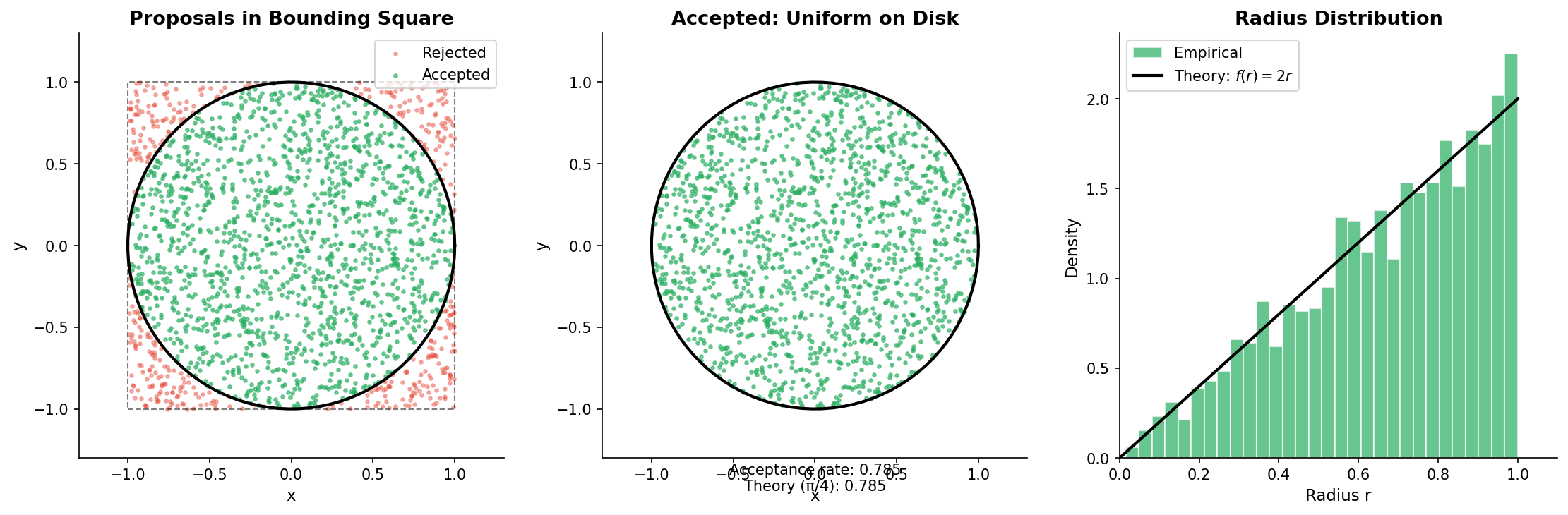
Fig. 2.37 Rejection Sampling for the Unit Disk. Blue points are accepted (inside disk); red points are rejected (in square corners). The acceptance rate equals the area ratio \(\pi/4 \approx 78.5\%\).
Worked Examples
We now apply rejection sampling to several important scenarios.
Example 1: Truncated Normal Distribution
A truncated normal distribution restricts the standard normal to an interval \([a, b]\). When \([a, b]\) lies in the tails, inversion methods become numerically unstable, but rejection sampling offers a simple solution.
Target: \(f(x) \propto \phi(x)\) for \(x \in [a, b]\)
Proposal: The untruncated normal \(g(x) = \phi(x)\)
Envelope: Since \(f(x) = \phi(x)\) when \(x \in [a, b]\) and 0 otherwise, we have \(f(x) \le g(x)\), so \(M = 1\).
Acceptance criterion: Accept \(X \sim \mathcal{N}(0, 1)\) if \(a \le X \le b\).
def truncated_normal(a, b, n_samples, seed=None):
    """
    Sample from N(0,1) truncated to [a, b] via rejection.

    Acceptance rate = Φ(b) - Φ(a).
    """
    rng = np.random.default_rng(seed)
    samples = []
    n_proposals = 0

    while len(samples) < n_samples:
        x = rng.standard_normal()
        n_proposals += 1
        if a <= x <= b:
            samples.append(x)

    theoretical_rate = stats.norm.cdf(b) - stats.norm.cdf(a)
    actual_rate = len(samples) / n_proposals

    return np.array(samples), actual_rate, theoretical_rate

# Example: truncate to [1, 3] (right tail)
samples, actual, theory = truncated_normal(1, 3, 10000, seed=42)
print(f"Truncated N(0,1) to [1, 3]:")
print(f"  Theoretical acceptance rate: {theory:.3%}")
print(f"  Actual acceptance rate: {actual:.3%}")
print(f"  Sample mean: {samples.mean():.4f}")
Output:
Truncated N(0,1) to [1, 3]:
  Theoretical acceptance rate: 15.7%
  Actual acceptance rate: 15.8%
  Sample mean: 1.5239
Common Pitfall ⚠️
Extreme truncation: If \([a, b]\) lies far in the tail (e.g., \([4, 6]\)), the acceptance rate becomes tiny: \(\Phi(6) - \Phi(4) \approx 0.003\%\). For extreme truncation, use specialized algorithms like Robert’s exponential tilting method or inverse CDF with careful numerical handling.
Example 2: Gamma Distribution
The Gamma distribution with non-integer shape parameter has no simple transformation from uniforms. Rejection sampling provides an efficient solution.
Target: \(\text{Gamma}(\alpha, 1)\) with \(\alpha > 0\)
For \(\alpha \ge 1\), Ahrens-Dieter and other algorithms use rejection with carefully chosen envelopes. Here’s a simplified version using an exponential proposal for \(\alpha \ge 1\):
def gamma_rejection(alpha, n_samples, seed=None):
    """
    Sample Gamma(alpha, 1) using rejection with exponential envelope.

    Uses the fact that for alpha >= 1, we can bound the Gamma density
    with a scaled exponential.
    """
    if alpha < 1:
        # Use transformation: Gamma(alpha) = Gamma(alpha+1) * U^(1/alpha)
        samples = gamma_rejection(alpha + 1, n_samples, seed)
        rng = np.random.default_rng(seed)
        u = rng.random(n_samples)
        return samples * u**(1/alpha)

    rng = np.random.default_rng(seed)

    # For alpha >= 1, use exponential(1/alpha) as proposal
    # Envelope constant derived from ratio at mode
    rate = 1 / alpha
    mode = alpha - 1

    # M = f(mode) / g(mode) where g is Exp(rate)
    f_mode = mode**(alpha - 1) * np.exp(-mode) / np.math.gamma(alpha)
    g_mode = rate * np.exp(-rate * mode)
    M = f_mode / g_mode * 1.01  # safety margin

    samples = []
    n_proposals = 0

    while len(samples) < n_samples:
        x = rng.exponential(1 / rate)  # Exp(rate) sample
        u = rng.random()
        n_proposals += 1

        # Gamma(alpha, 1) pdf (up to constant)
        f_x = x**(alpha - 1) * np.exp(-x)
        # Exp(rate) pdf
        g_x = rate * np.exp(-rate * x)

        if u <= f_x / (M * g_x):
            samples.append(x)

    print(f"Gamma({alpha}): acceptance rate = {len(samples)/n_proposals:.1%}")
    return np.array(samples)

# Test
samples = gamma_rejection(2.5, 10000, seed=42)
print(f"Sample mean: {samples.mean():.3f} (theory: 2.5)")
print(f"Sample var:  {samples.var():.3f} (theory: 2.5)")
Example 3: Custom Posterior Distribution
Rejection sampling shines in Bayesian inference where posteriors are known only up to proportionality.
Scenario: Binomial likelihood with Beta prior yields Beta posterior, but suppose we want to apply rejection sampling without recognizing the conjugate form.
def bayesian_posterior_rejection(n_successes, n_trials, prior_alpha, prior_beta,
                                 n_samples, seed=None):
    """
    Sample from posterior of Binomial parameter θ.

    Prior: θ ~ Beta(prior_alpha, prior_beta)
    Likelihood: X | θ ~ Binomial(n_trials, θ)
    Posterior: θ | X ∝ θ^(α + x - 1) (1-θ)^(β + n - x - 1)
    """
    # Posterior kernel (unnormalized)
    def posterior_kernel(theta):
        if theta <= 0 or theta >= 1:
            return 0.0
        return (theta**(prior_alpha + n_successes - 1) *
                (1 - theta)**(prior_beta + n_trials - n_successes - 1))

    # Use uniform proposal on [0, 1]
    x_grid = np.linspace(0.001, 0.999, 1000)
    kernel_vals = [posterior_kernel(x) for x in x_grid]
    M = max(kernel_vals) * 1.01

    rng = np.random.default_rng(seed)
    samples = []
    n_proposals = 0

    while len(samples) < n_samples:
        theta = rng.random()  # Uniform(0, 1)
        u = rng.random()
        n_proposals += 1

        if u <= posterior_kernel(theta) / M:
            samples.append(theta)

    return np.array(samples), n_samples / n_proposals

# Example: 7 successes in 10 trials, uniform prior
samples, acc_rate = bayesian_posterior_rejection(
    n_successes=7, n_trials=10,
    prior_alpha=1, prior_beta=1,  # uniform prior
    n_samples=10000, seed=42
)

# True posterior is Beta(8, 4)
print(f"Posterior mean: {samples.mean():.4f} (theory: {8/12:.4f})")
print(f"Acceptance rate: {acc_rate:.1%}")
Limitations and the Curse of Dimensionality
Rejection sampling is elegant and exact, but it has fundamental limitations.
The High-Dimensional Problem
In \(d\) dimensions, the envelope condition becomes:
The acceptance probability is still \(1/M\), but now \(M\) often grows exponentially with dimension.
Example: Target is \(\mathcal{N}(\mathbf{0}, \mathbf{I}_d)\) and proposal is \(\mathcal{N}(\mathbf{0}, \sigma^2 \mathbf{I}_d)\) with \(\sigma > 1\). The ratio \(f(\mathbf{x})/g(\mathbf{x})\) involves:
The maximum occurs at \(\mathbf{x} = \mathbf{0}\), giving \(M = \sigma^d\). For \(\sigma = 1.5\) and \(d = 20\), this is \(1.5^{20} \approx 3,300\)—a 0.03% acceptance rate!
When Rejection Sampling Fails
Rejection sampling becomes impractical when:
High dimensions: The curse of dimensionality makes finding a tight envelope nearly impossible.
Multimodal targets: A single proposal struggles to cover well-separated modes without huge \(M\).
Heavy tails with light-tailed proposals: If \(f(x)/g(x) \to \infty\) as \(|x| \to \infty\), no finite \(M\) exists.
Unknown mode location: Without knowing where the target is concentrated, any proposal is a guess.
Practical guideline: Rejection sampling works well for \(d \le 5\) or so. For higher dimensions, consider Markov Chain Monte Carlo (Metropolis-Hastings, Gibbs sampling) which we develop in later chapters.
Connections to Other Methods
Rejection sampling is the ancestor of several more sophisticated techniques.
Importance Sampling
Where rejection sampling discards proposals that don’t pass the acceptance test, importance sampling keeps all proposals but assigns them weights:
Expectations are then computed as weighted averages. Importance sampling avoids discarding samples but requires careful handling of weight variability. We develop this in detail in ch2.6-variance-reduction.
Markov Chain Monte Carlo
The Metropolis-Hastings algorithm generalizes rejection sampling to create a Markov chain whose stationary distribution is the target. Instead of independent proposals, it uses sequential proposals from a transition kernel. Rejected proposals don’t disappear—the chain stays at its current position. This modification allows MCMC to work efficiently in high dimensions where direct rejection sampling fails. See Chapter 5 for full development.
Adaptive Rejection Sampling
For log-concave densities (densities \(f(x)\) where \(\log f(x)\) is concave), the ARS algorithm of Gilks and Wild (1992) constructs an envelope adaptively during sampling. The key insight is that tangent lines to a concave function lie above the function, while secant lines lie below.
Log-concave examples: Many important distributions are log-concave:
Normal: \(\log \phi(x) \propto -x^2/2\) (concave parabola)
Exponential: \(\log(\lambda e^{-\lambda x}) \propto -\lambda x\) (linear, hence concave)
Gamma with \(\alpha \ge 1\): \(\log f(x) \propto (\alpha-1)\log x - x\) (concave for \(\alpha \ge 1\))
Beta with \(\alpha, \beta \ge 1\): log-concave on \((0, 1)\)
Logistic, log-normal truncated appropriately
The ARS algorithm:
Initialize with a few points \(S_n = \{x_0, x_1, \ldots, x_n\}\) where \(\log f(x_i)\) is known.
Construct upper envelope \(\bar{h}_n(x)\): piecewise linear, connecting tangent lines at \(x_i\). By concavity, this lies above \(\log f(x)\).
Construct lower envelope \(\underline{h}_n(x)\): piecewise linear through \((x_i, \log f(x_i))\). By concavity, this lies below \(\log f(x)\).
Sample from \(g_n(x) \propto \exp(\bar{h}_n(x))\) (piecewise exponential, easy to sample).
Squeeze test: If \(U \le \exp(\underline{h}_n(X) - \bar{h}_n(X))\), accept immediately.
Full test: Otherwise, evaluate \(f(X)\) and accept if \(U \le f(X)/g_n(X)\).
Adapt: If rejected (or if \(f(X)\) was evaluated), add \(X\) to \(S_n\), tightening future envelopes.
The adaptive nature means efficiency improves as sampling progresses—early rejections contribute information that speeds later sampling. ARS is particularly valuable within Gibbs samplers where full conditionals are often log-concave.
Limitation: ARS requires log-concavity. For non-log-concave targets (e.g., mixture distributions, heavy-tailed posteriors), the algorithm fails. The ARMS extension (Adaptive Rejection Metropolis Sampling) handles non-log-concave targets by adding a Metropolis-Hastings correction step.
Practical Considerations
Numerical Stability
Several numerical issues can arise:
Underflow in density ratios: When \(f(x)\) is very small, \(f(x)/[M \cdot g(x)]\) may underflow to zero. Work with log-densities: accept if \(\log U \le \log f(x) - \log M - \log g(x)\).
Overflow in unnormalized densities: Large exponents can overflow. Again, log-densities help.
Zero proposal density: If \(g(x) = 0\) at a point where \(f(x) > 0\), the ratio is undefined. Ensure proposal support covers target support.
Log-space implementation for numerical stability:
def rejection_sample_log(log_target, log_proposal, proposal_sampler,
                         log_M, n_samples, seed=None):
    """
    Rejection sampling using log-densities for numerical stability.

    Accept if log(U) <= log_target(x) - log_M - log_proposal(x)
    """
    rng = np.random.default_rng(seed)
    samples = []

    while len(samples) < n_samples:
        x = proposal_sampler(rng)
        log_u = np.log(rng.random())  # log(U) where U ~ Uniform(0,1)

        log_accept_prob = log_target(x) - log_M - log_proposal(x)

        if log_u <= log_accept_prob:
            samples.append(x)

    return np.array(samples)
This approach handles densities that would otherwise cause overflow or underflow in direct computation.
Verifying Correctness
Always verify your rejection sampler:
Check acceptance rate: Compare actual rate to theoretical \(1/M\).
Compare moments: Sample mean and variance should match theoretical values.
Visual comparison: Histogram of samples should match theoretical density.
Kolmogorov-Smirnov test: Statistical test for distribution match.
def verify_rejection_sampler(samples, true_dist, name=""):
    """Verify rejection samples against known distribution."""
    # Moments
    print(f"{name} verification:")
    print(f"  Sample mean: {samples.mean():.4f}, Theory: {true_dist.mean():.4f}")
    print(f"  Sample std:  {samples.std():.4f}, Theory: {true_dist.std():.4f}")

    # KS test
    ks_stat, p_value = stats.kstest(samples, true_dist.cdf)
    print(f"  KS statistic: {ks_stat:.4f}, p-value: {p_value:.4f}")

    if p_value < 0.01:
        print("  WARNING: KS test suggests samples may not match target!")
Production Diagnostics
For production use, a sampler with built-in monitoring helps detect issues:
class RejectionSamplerWithDiagnostics:
    """Rejection sampler with performance monitoring."""

    def __init__(self, target_pdf, proposal_sampler, proposal_pdf, M):
        self.target_pdf = target_pdf
        self.proposal_sampler = proposal_sampler
        self.proposal_pdf = proposal_pdf
        self.M = M

        # Diagnostics
        self.n_proposed = 0
        self.n_accepted = 0
        self.acceptance_history = []

    def sample(self, size, batch_size=100, seed=None):
        """Sample with batch monitoring."""
        rng = np.random.default_rng(seed)
        samples = []

        while len(samples) < size:
            batch_accepted = 0

            for _ in range(min(batch_size, size - len(samples) + 100)):
                y = self.proposal_sampler(rng)
                self.n_proposed += 1

                u = rng.random()
                accept_prob = self.target_pdf(y) / (self.M * self.proposal_pdf(y))

                if u <= accept_prob:
                    samples.append(y)
                    self.n_accepted += 1
                    batch_accepted += 1

                    if len(samples) >= size:
                        break

            # Record batch acceptance rate
            if batch_size > 0:
                self.acceptance_history.append(batch_accepted / batch_size)

        return np.array(samples[:size])

    def get_diagnostics(self):
        """Return sampling diagnostics."""
        actual_rate = self.n_accepted / self.n_proposed if self.n_proposed > 0 else 0
        return {
            'n_proposed': self.n_proposed,
            'n_accepted': self.n_accepted,
            'actual_acceptance_rate': actual_rate,
            'theoretical_rate': 1 / self.M,
            'efficiency': actual_rate * self.M,  # Should be ≈ 1
            'acceptance_history': self.acceptance_history
        }
The efficiency metric should be close to 1.0; significant deviations indicate either an incorrect \(M\) or implementation bugs.
Try It Yourself 🖥️
Exercise 1: Semicircle Distribution
The semicircle distribution has density \(f(x) = \frac{2}{\pi}\sqrt{1 - x^2}\) for \(x \in [-1, 1]\). Implement rejection sampling with a uniform proposal. What is the theoretical acceptance rate? Verify your implementation by comparing sample moments to the theoretical mean (0) and variance (\(1/4\)).
Exercise 2: Optimal Proposal for Gamma
For \(\text{Gamma}(\alpha, 1)\) with \(\alpha = 0.5\), try both (a) an exponential proposal and (b) a Weibull proposal. Which achieves a higher acceptance rate? Hint: For small \(\alpha\), the Gamma density has a singularity at 0.
Exercise 3: Bivariate Rejection
Implement rejection sampling for the bivariate distribution with density proportional to \(\exp(-(x^2 + y^2 + xy))\) using a bivariate normal proposal. Estimate \(M\) numerically and compare theoretical vs. actual acceptance rates.
Exercise 4: Envelope Violation Detection
Write a diagnostic function that detects when \(M\) is too small (envelope violation). The function should sample points and flag any where \(f(x) > M \cdot g(x)\). Test it on Beta(0.5, 0.5) with a uniform proposal and varying \(M\).
Exercise 5: von Mises (Circular Normal) Distribution
The von Mises distribution has PDF \(f(\theta) = \frac{e^{\kappa \cos(\theta - \mu)}}{2\pi I_0(\kappa)}\) for \(\theta \in [0, 2\pi)\), where \(I_0\) is the modified Bessel function. Implement rejection sampling using a Uniform \([0, 2\pi)\) proposal. Plot acceptance rate as a function of concentration parameter \(\kappa\) for \(\kappa \in \{0.5, 1, 2, 5, 10\}\). Why does efficiency degrade as \(\kappa\) increases?
Bringing It All Together
Rejection sampling provides a universal method for generating random samples from any distribution whose density we can evaluate pointwise. The key insights are:
Geometric foundation: Points uniformly distributed under a density curve have \(x\)-coordinates following that density. Rejection sampling implements this by filtering proposals.
Envelope requirement: We need \(f(x) \le M \cdot g(x)\) everywhere. The constant \(M\) determines efficiency through acceptance rate \(1/M\).
Normalization not required: The algorithm works even when \(f(x)\) is known only up to a constant—essential for Bayesian posterior sampling.
Proposal design matters: Good proposals have similar shape to the target. Tail behavior is critical: light-tailed proposals for heavy-tailed targets fail.
Dimensional limitations: Acceptance rates degrade exponentially with dimension. For \(d \gtrsim 5\), consider MCMC alternatives.
Foundation for advanced methods: Rejection sampling’s ideas appear in importance sampling, Metropolis-Hastings, and adaptive rejection sampling.
Looking Ahead
The next section introduces variance reduction techniques that improve Monte Carlo efficiency. Some, like importance sampling, can be viewed as alternatives to rejection sampling that use all proposals rather than discarding rejects. Others, like antithetic variates and control variates, reduce estimator variance through clever correlation structures.
Key Takeaways 📝
The algorithm: Propose from \(g(x)\), accept with probability \(f(x)/[M \cdot g(x)]\). Accepted samples are exact draws from \(f\).
Envelope condition: Must have \(f(x) \le M \cdot g(x)\) for all \(x\). Violation produces biased samples—a silent error.
Efficiency = 1/M: Expected proposals per accepted sample equals \(M\). Tight envelopes (small \(M\)) are crucial for efficiency.
Normalization not needed: The algorithm works for unnormalized densities—essential for Bayesian inference where \(p(\theta|x) \propto p(x|\theta)p(\theta)\).
Proposal design: Match proposal tails to target tails. Support of \(g\) must cover support of \(f\). For bounded support, uniform proposals often suffice.
Curse of dimensionality: Acceptance rates degrade exponentially with dimension. Practical limit is roughly \(d \le 5\).
Outcome alignment: Rejection sampling (Learning Outcome 1) enables exact sampling from complex distributions. Understanding its limitations motivates MCMC methods developed later in the course.